An Operational Optimization Model for Micro Energy Grids in Photovoltaic-Storage Agricultural Greenhouses Based on Operation Mode Selection

Abstract

Addressing the urgent need for sustainable energy transitions in rural development while achieving the dual carbon goals, this study focuses on resolving critical challenges in agricultural photovoltaic (PV) applications, including land-use conflicts, compound energy demands (electricity, heating, cooling), and financial constraints among farmers. To tackle these issues, a dual-mode cost–benefit analysis framework was developed, integrating two distinct investment models: self-invested construction (SIC), where farmers independently finance and manage the system, and energy performance contracting (EPC), where third-party investors fund infrastructure through shared energy-saving or revenue agreements. Then, an integrated photovoltaic-storage agricultural greenhouse (PSAG) microgrid optimization model is established, synergizing renewable energy generation, battery storage, and demand-side management while incorporating operational mode selection. The proposed model is validated through a real-world case study of a village agricultural greenhouse in Gannan, China, characterized by typical rural energy profiles and climatic conditions. Simulation results demonstrate that the optimal system configuration requires 27.91 kWh energy storage capacity and 18.67 kW peak output, with annualized post-depreciation costs of 81,083.69 yuan (SIC) and 74,216.22 yuan (EPC). The key findings reveal that energy storage integration reduces operational costs by 8.5% compared to non-storage scenarios, with the EPC model achieving 9.3% greater cost-effectiveness than SIC through shared-investment mechanisms. The findings suggest that incorporating an energy storage system reduces costs for farmers, with the EPC model offering greater cost savings.

1. Introduction

Electricity for agricultural production constitutes a significant portion of today’s energy consumption; however, the current utilization of renewable energy in this sector remains low, with a heavy reliance on fossil fuels [1,2]. The prioritization of power supply infrastructure is urgently required for China’s agricultural development [3]. Rural areas in China are vast and often possess abundant renewable resources, such as solar, wind, hydro, and biomass [4,5]. Under the Fourteenth Five-Year Plan, China’s rural energy transition will focus on the local development of clean energy sources, including solar energy and biomass, to meet the demand for clean electricity in rural production and living. Greenhouses are essential for modernizing agricultural production, and China has an extensive range of greenhouse areas [6,7]. These greenhouses can be outfitted with energy storage devices and integrated with photovoltaic (PV) systems to enhance their operational controllability [8].

Recent advancements in rural energy systems have demonstrated significant progress in optimizing economic and environmental performance through diverse methodological approaches. Zhu et al. [9] employed interval linear programming to optimize a remote rural distributed renewable energy system design, demonstrating that the carbon reduction rate could reach 4.0–49.6%. Yang et al. [10] proposed a new rural energy microgrid structure based on biomass fuel and designed a two-stage dispatch optimization framework, which revealed that clean energy consumption improved through optimization. In terms of energy storage integration, Güven et al. [11] developed a clean energy system that converted surplus electricity into hydrogen energy storage, achieving greater utilization of renewable energy. Kamal et al. [12,13] developed an off-grid microgrid for rural India and optimized it via differential evolution to address cost and intermittency challenges. In terms of algorithm optimization, Suman et al. [14] optimized a rural microgrid with solar/wind/bio-generator/diesel/battery through the PSO-GWO method, which effectively reduced the cost of electricity and the deficiency of power supply probability. Chen et al. [15] proposed a Wasserstein distance-based distributed robust optimal scheduling model for rural microgrids considering the collaborative interaction of source–grid–load–storage, which effectively reduces the operating costs of rural microgrids. Subhash et al. [16] optimized the design of isolated microgrids based on hybrid renewable energy systems to minimize the net present cost and energy cost while ensuring system reliability. While these studies have developed integrated energy systems tailored to the characteristics of rural supply and demand, their practical applications in agricultural greenhouses remains underexplored.

Recent advancements in PV agricultural greenhouses have primarily focused on technological integration and energy efficiency optimization. Boccalatte et al. [17] pioneered a translucent roof-mounted PV greenhouse (3 kWh) integrated with heat pumps, achieving Near Zero Energy Building status. Azam et al. [18] developed a hybrid solar-powered greenhouse dryer for tomato post-harvest processing, combining PV with thermal energy collection and computational modeling to assess thermal efficiency. Zahra et al. [19] and Yao et al. [20] advanced structural and lighting optimization, with the former integrating energy, crop growth, and solar panel models for unevenly structured greenhouses, and the latter employing RADIANCE simulations for vertical cultivation. In terms of system innovation, Ghiasi et al. [21] integrated geothermal and PV into rural greenhouse heating systems to improve efficiency and achieve sustainable agricultural development. Wang [22] and Fatemeh et al. [23] conducted a full life cycle assessment and management of energy consumption in agricultural PV greenhouses, which helped to promote agricultural energy optimization and improve resource utilization efficiency. To enhance the overall performance of PV output prediction models, Zhu et al. [24] proposed forecasting models for solar irradiance time series, including Pyraformer, Informer, Transformer, and TimesNet, and analyzed the models that are most suitable for various scenarios under real-world conditions. Although these studies have significantly advanced the technical integration and energy efficiency of PV agricultural greenhouses, there is a lack of research on the operation optimization of the economic benefits of photovoltaic agricultural greenhouses from the perspective of operation models, as shown in

Table 1. Comparative analysis of PV agricultural greenhouse research.

Reference	Key Focus	Methodology	Economic Optimization	Operational Mode Analysis
Boccalatte et al. [17]	NZEB design	PV–heat pump integration	Energy efficiency metrics	no
Azam et al. [18]	Post-harvest drying	Hybrid PV–thermal system	Thermal efficiency analysis	no
Zahra et al. [19]	Structural-energy balance	Energy–growth–PV coupling	Yield–energy trade-offs	no
Yao et al. [20]	Lighting optimization	RADIANCE lighting simulation	Spatial efficiency metrics	no
Ghiasi et al. [21]	Geothermal–PV hybrid	Hybrid heating system Design	Sustainability assessment	no
Wang et al. [22]	Lifecycle energy management	LCA framework	Resource utilization efficiency	no
Zhu et al. [24]	PV forecasting	Solar irradiance time series	Prediction accuracy improvement	no
This study	Operational economics	Dual-mode robust optimization (SIC/EPC)	Cost–benefit trade-offs under financial models	yes

.

In order to bridge the gaps identified in Table 1 and examine the economic benefits of photovoltaic-storage agricultural greenhouses (PSAGs), this paper proposes a novel microgrid framework that synergistically integrates PV systems, energy storage, and agricultural facilities, explicitly addressing PV generation uncertainties. Then, dual-mode cost–benefit models incorporating self-invested construction (SIC) and energy performance contracting (EPC) frameworks are established. Finally, based on the scenario optimization method, the optimal three-day operation strategy and energy storage capacity are obtained through three representative daily load curves, so as to compare and determine the most effective operation mode.

2. Photovoltaic-Storage Agricultural Greenhouse Micro Energy Grid Model

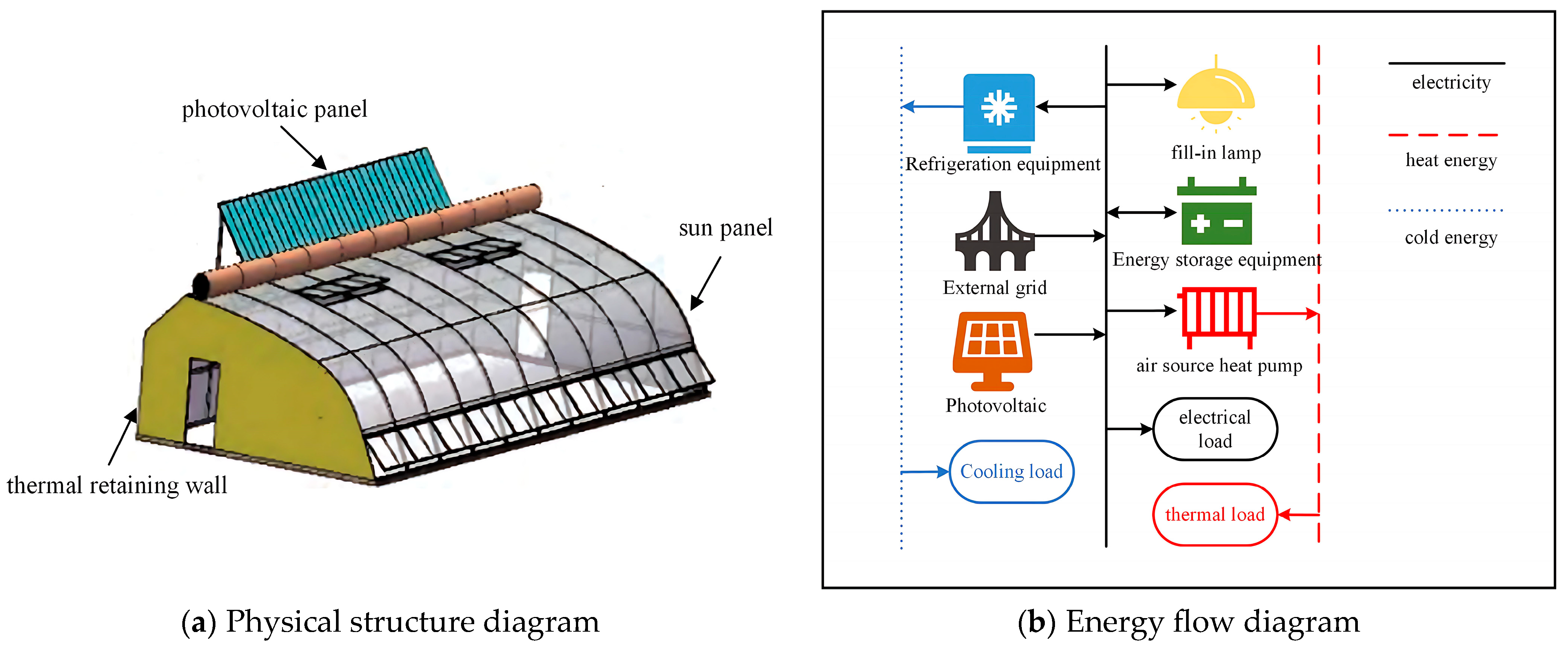
2.1. Physical Structure of Photovoltaic-Storage Agricultural Greenhouses

The PSAG micro energy grid primarily consists of PV power generation devices and agricultural greenhouse power systems. Specifically, it includes PV panels, air-source heat pumps, refrigeration units, energy storage systems, and other agricultural facilities. The physical structure and energy flow of the agro-optical complementary agricultural greenhouses are depicted in Figure 1.

Agricultural greenhouses operations demand a controlled environment that uses air-source heat pumps for the necessary heat load, refrigeration units for the cooling load, and artificial lighting for the supplemental lighting needs.

2.2. Photovoltaic Power Generation System Model

The electrical output of PV depends on factors such as solar irradiance and ambient temperature. According to relevant studies, PV power generation follows a beta distribution over a specified period [25]. The output power is represented in Equation (1):

$$P_{\mathrm{pv}}=rA\eta {\displaystyle \sum _{i=1}^n{X}_i{Y}_i}$$

(1)

where r is the solar light intensity, A is the total PV panels surface, and η is the conversion efficiency. The sunlight intensity follows a beta distribution, and its probability density function can be expressed as Equation (2):

$$f(r)=\frac{\mathrm{\Gamma }(\alpha +\beta )}{\mathrm{\Gamma }(\alpha )\mathrm{\Gamma }(\beta )}{(\frac{r}{{\mathrm{r}}_{\max }})}^{\alpha -1}{(1-\frac{r}{{\mathrm{r}}_{\max }})}^{\beta -1}$$

(2)

where $r_{\max }$ is the maximum intensity of light radiation, $\alpha$ and $\beta$ are the beta distribution parameters, and $\mathrm{\Gamma }$ is the gamma function.

The magnitude of $\eta$ is related to the ambient temperature, as shown in Equation (3):

$$\eta ={\eta }_0(1+k(T-T_0))$$

(3)

where ${\eta }_0$ is the conversion efficiency at standard conditions; the conversion efficiency is taken in the case of 25 °C. $k$ is the temperature effect coefficient and $T_0$ takes the value of 25 °C.

From the above equation, the average value of the PV output power at that moment can be found, as shown in Equation (4):

$$P_{\mathrm{pv}}={\displaystyle \int rA}{\eta }_0(1+k(T-{\mathrm{T}}_0))\ast \frac{\mathrm{\Gamma }(\alpha +\beta )}{\mathrm{\Gamma }(\alpha )\mathrm{\Gamma }(\beta )}(\frac{r}{r_{\max }}{)}^{\alpha -1}{(1-\frac{r}{r_{\max }})}^{\beta -1}$$

(4)

2.3. Energy Storage System Model

The energy storage system in this study is primarily composed of electrochemical energy storage, which is mathematically modeled as Equation (5):

$$E(t)=E(t-1)(1-\alpha )+\Delta t{P}_{\mathrm{ch}}(t){\beta }_{\mathrm{ch}}-\Delta t{P}_{\mathrm{dis}}(t)/{\beta }_{\mathrm{dis}}$$

(5)

where $E\left(t\right)$ is the amount of electricity in the storage unit at time t. $E(t-1)$ represents the quantity of electricity within the energy storage apparatus at time t − 1. $\alpha$ represents the self-discharge factor of the energy storage system, with a value fixed at 0.05. $\Delta t$ represents the unit time. $P_{\mathrm{ch}}(t)$ represents power during the charging process of the energy storage system at time t. ${\beta }_{\mathrm{ch}}$ is the charging efficiency factor of the energy storage system and takes a value of 0.95. $P_{\mathrm{dis}}(t)$ represents the discharge power that energy storage outputs at time t. ${\beta }_{\mathrm{dis}}$ represents the discharge efficiency factor of the energy storage system and takes a value of 0.95.

2.4. Agricultural Greenhouse Heating Model

Heating agricultural greenhouses is essential for protecting crops during the winter months. This study employs the air-source heat pump (ASHP) method. It functions based on the principle of leveraging energy-efficient equipment to convey heat from a low-temperature reservoir to a high-temperature one. This equipment is both low in pollution and economically and environmentally advantageous. The mathematical formula for this process is presented in Equation (6):

$$Q_{\mathrm{HP}}\left(t\right)=C_{\mathrm{HP}}{P}_{\mathrm{EHP}}\left(t\right)$$

(6)

where $Q_{\mathrm{HP}}(t)$ represents the heating power of the ASHP at time t. $C_{\mathrm{HP}}$ represents the heating coefficient of ASHP and takes a value of 3.7. $P_{\mathrm{EHP}}(t)$ represents the electrical power used by the ASHP at time t.

2.5. Agricultural Greenhouse Cooling Model

Cooling agricultural greenhouses is crucial during the summer months to maintain crop viability. In this study, a similar method using ASHP is applied to calculate the cooling power, and it is mathematically represented as Equation (7):

$$Q_{\mathrm{CP}}\left(t\right)=C_{\mathrm{CP}}{P}_{\mathrm{ECP}}\left(t\right)$$

(7)

where $Q_{\mathrm{CP}}(t)$ represents the cooling power of the refrigeration unit at time t. $C_{\mathrm{CP}}$ represents its cooling factor and takes a value of 3.5. $P_{\mathrm{ECP}}(t)$ is the electrical power used by the refrigeration unit.

2.6. Robust Optimization Model for Photovoltaic Output Uncertainty

The deviation of actual PV output from the forecasted output is attributed to uncertainties. The actual output can be expressed using the following formulas [26,27]:

$$\left\{\begin{array}{l}{P}_{\mathrm{pv}}^t=P_{\mathrm{pv}}^{\prime t}+\Delta P_{\mathrm{pv}}^t\\ P_{\mathrm{pv}}^{\mathrm{ld}}\le \Delta P_{\mathrm{pv}}^t\le P_{\mathrm{pv}}^{\mathrm{ud}}\\ P_{\mathrm{supply}}^t-P_{\mathrm{demand}}^t=\max \{-P_{\mathrm{pv}}^t\}=-P_{\mathrm{pv}}^{\prime t}+\max \{-{\eta }_{\mathrm{pv}}^{\mathrm{ld}}{P}_{\mathrm{pv}}^{\mathrm{ld}}-{\eta }_{\mathrm{pv}}^{\mathrm{ud}}{P}_{\mathrm{pv}}^{\mathrm{ud}}\}\\ {\eta }_{\mathrm{pv}}^{\mathrm{ld}}+{\eta }_{\mathrm{pv}}^{\mathrm{ud}}\le {\mathrm{\Gamma }}_{\mathrm{pv}}^t\\ 0\le {\eta }_{\mathrm{pv}}^{ld},{\eta }_{\mathrm{pv}}^{\mathrm{ud}}\le 1\end{array}\right.$$

(8)

where $P_{\mathrm{pv}}^t$ is actual output of PV. $P_{\mathrm{pv}}^{\prime t}$ is the forecasted output of PV. $\Delta P_{\mathrm{pv}}^t$ is the fluctuating range for PV output. $P_{\mathrm{pv}}^{\mathrm{ld}}$ and $P_{\mathrm{pv}}^{\mathrm{ud}}$ are the upper and lower limits of the volatility range, respectively. $P_{\mathrm{supply}}^t$ represents the electric power supply at time t except for PV. $P_{\mathrm{demand}}^t$ represents the electricity demand excluding PV at time t. ${\eta }_{\mathrm{pv}}^{\mathrm{ld}}$ and ${\eta }_{\mathrm{pv}}^{\mathrm{ud}}$ are PV output fluctuation range output deviations. ${\mathrm{\Gamma }}_{\mathrm{pv}}^t$ is the degree of uncertainty in PV output.

By decomposing the inner and outer layers, the worst case of PV output is represented by Equation (9):

$$\left\{\begin{array}{l}\mathrm{Max}\{-{\eta }_{\mathrm{pv}}^{\mathrm{ld}}{P}_{\mathrm{pv}}^{\mathrm{ld}}-{\eta }_{\mathrm{pv}}^{\mathrm{ud}}{P}_{\mathrm{pv}}^{\mathrm{ud}}\}\\ {\eta }_{\mathrm{pv}}^{\mathrm{ld}}+{\eta }_{\mathrm{pv}}^{\mathrm{ud}}\le {\mathrm{\Gamma }}_{\mathrm{pv}}^t\\ 0\le {\eta }_{\mathrm{pv}}^{\mathrm{ld}}{P}_{\mathrm{pv}}^{\mathrm{ld}},{\eta }_{\mathrm{pv}}^{\mathrm{ud}}{P}_{\mathrm{pv}}^{\mathrm{ud}}\le 1\end{array}\right.$$

(9)

By introducing the dyadic variables ${\lambda }_{\mathrm{pv}}^t$, ${\pi }_{\mathrm{pv}}^{t+}$, and ${\pi }_{\mathrm{pv}}^{t-}$, the above equation can be transformed to Equation (10):

$$\left\{\begin{array}{l}\min \{{\lambda }_{\mathrm{pv}}^t{\mathrm{\Gamma }}_{\mathrm{pv}}^t+{\pi }_{\mathrm{pv}}^{t+}+{\pi }_{\mathrm{pv}}^{t-}\}\\ {\lambda }_{\mathrm{pv}}^t+{\pi }_{\mathrm{pv}}^{t-}\ge -P_{\mathrm{pv}}^{\mathrm{ld}},{\lambda }_{\mathrm{pv}}^t+{\pi }_{\mathrm{pv}}^{t+}\ge -P_{\mathrm{pv}}^{\mathrm{ud}}\\ {\pi }_{\mathrm{pv}}^{t+},{\pi }_{\mathrm{pv}}^{t-}\ge 0\end{array}\right.$$

(10)

From the dyadic principle, it can be seen that the original problem for robust optimization of PV output can be equated to the worst-case PV output model.

$$P_{\mathrm{supply}}^t-P_{\mathrm{demand}}^t=-P_{\mathrm{pv}}^{\prime t}+{\lambda }_{\mathrm{pv}}^t{\mathrm{\Gamma }}_{\mathrm{pv}}^t+{\pi }_{\mathrm{pv}}^{t+}+{\pi }_{\mathrm{pv}}^{t-}$$

(11)

2.7. Load Model of Micro Energy Grids for PSAG

In this study, the architectural configuration of the PSAG for greenhouse applications is schematically presented in Figure 1. The heating and cooling loads are comparable, and their functions are analogous; therefore, a unified mathematical model is employed, as represented in the following equation [28]:

$$Q_{\mathrm{dp}}=Q_1+Q_2+Q_3=\sum s_j{a}_j\left(\left|t_{\mathrm{in}}-t_{\mathrm{out}}\right|\right)+0.5kvn\left(\left|t_{\mathrm{in}}-t_{\mathrm{out}}\right|\right)+\sum z_1{h}_1\left(\left|t_{\mathrm{in}}-t_{\mathrm{out}}\right|\right)$$

(12)

where $Q_{\mathrm{dp}}$ is the total cooling and heating power required. $Q_1$ represents the wall heat transfer load. $Q_2$ represents the air infiltration heat transfer load. $Q_3$ represents the ground heat transfer load. $s_j$ represents the heat transfer coefficient of the jth wall structure. This investigation prioritizes the thermal conductivity parameters of roof-mounted PV panels and insulated wall assemblies within the shed structure, which are taken as 3.4 W/m²·k and 0.622 W/m²·k, respectively. $a_j$ represents the area of the jth wall structure, which is taken as 912 m² and 170 m², respectively. $k$ represents the wind factor and takes the value of 1. $v$ represents the total air volume in the greenhouse and takes the value of 1360 m³. $n$ represents the number of air changes per unit of time and takes the value of 1.2. $z_1$ represents the ground heat transfer coefficient and takes the value of 0.24 w/m²·k. $h_1$ represents the total surface area and takes the value of 720 m². $t_{\mathrm{in}}$ represents the temperature within the greenhouse. $t_{\mathrm{out}}$ represents the outdoor temperature.

Furthermore, this paper considers the load needed to produce light at night for 8 h. The load power is $P_{\mathrm{G}}$. It fulfils the following conditions:

$${\displaystyle \sum }_{t=8}^{t=18}Tem{p}_{\mathrm{G}}\left(1,t\right)=0$$

(13)

$${\displaystyle \sum }_{t=8}^{t=18}Tem{p}_{\mathrm{G}}\left(1,t\right)=0$$

(14)

$$P_{\mathrm{G}}=Tem{p}_{\mathrm{G}}\ast a$$

(15)

where $Tem{p}_{\mathrm{G}}$ is a variable indicating whether the light is currently being produced, with values of 1 for yes and 0 for no. $P_G$ is the produced light load. $a$ is the produced light load value.

Time-shiftable load modeling for PSAG is shown in Equations (16) and (17):

$$P_{\mathrm{after}}\left(t\right)=P_{\mathrm{before}}\left(t\right)+P_{\mathrm{in}}\left(t\right)+P_{\mathrm{out}}\left(t\right)$$

(16)

$${\displaystyle \sum }_{t=1}^T{P}_{\mathrm{after}}\left(t\right)={\displaystyle \sum }_{t=1}^T{P}_{\mathrm{fore}}\left(t\right)$$

(17)

where $P_{\mathrm{after}}\left(t\right)$ represents the load state after transfer. $P_{\mathrm{before}}\left(t\right)$ is the load state before the transfer. $P_{\mathrm{in}}\left(t\right)$ represents the load transferred at time t. $P_{\mathrm{out}}\left(t\right)$ represents the load transferred at time t. The total time-shiftable load is a constant value.

2.8. Carbon Emission Model

2.8.1. Carbon Emission Reduction Model for PV Power Generation

PV power systems markedly lower carbon emissions while reducing fossil fuel dependency, yielding significant ecological advantages. The calculation of these reductions can derive from the Ministry of Ecology and Environment standards, as illustrated in China’s regional power grid baseline emission factors, as shown in Equation (18):

$$E_{\mathrm{F}}=0.75\times E_{\mathrm{FOM}}+0.25\times E_{\mathrm{FBM}}$$

(18)

where $E_{\mathrm{F}}$ is the grid baseline emission factor. $E_{\mathrm{FOM}}$ denotes the electricity marginal emission factor and takes the value of 0.9417. $E_{\mathrm{FBM}}$ is the capacity marginal emission factor and takes the value of 0.4819.

2.8.2. Grid Carbon Model

Carbon emissions from purchased electricity for agricultural greenhouses are part of their indirect carbon emissions [29], which are shown in Equation (19):

$$V_{\mathrm{C}{\mathrm{O}}_2\text{-}\mathrm{buy}}=E_{\mathrm{F}}\times E_{\mathrm{buy}}$$

(19)

where $V_{\mathrm{C}{\mathrm{O}}_2\text{-}\mathrm{buy}}$ is carbon emissions for purchased electricity. $E_{\mathrm{buy}}$ is purchased electricity.

3. Operational Optimization Model Based on the Selection of Project Operating Mode

3.1. Analysis of Different Project Operation Modes

This study examines the advantages and disadvantages of two project operation modes: self-invested construction (SIC) and contract management (energy performance contracting, EPC).

Under the SIC model, property rights are held by the farmer, who is responsible for both profits and losses. The farmer also reaps the environmental benefits from residual on-grid revenue and carbon emission reductions. Additionally, the farmer bears the investment-related costs, operation, and maintenance of the PV and storage systems, as well as the expenses related to purchasing electricity from the grid. In contrast, under the EPC model, property rights are owned by the PV investing enterprise. The farmer benefits from a preferential tariff on PV power generation and receives rental income.

In both modes, agricultural greenhouses must make decisions regarding the purchase, sale, and storage of electricity, ensuring that electricity demand is consistently met at all times to achieve optimal costs.

3.2. Cost–Benefit Analysis of Different Project Operating Modes

3.2.1. Cost–Benefit Analysis Under the SIC Mode

Under the SIC mode, it is necessary to consider the annual maintenance costs, PV power generation revenues, PV power generation carbon trading revenues, power purchase costs, and initial investment costs. The cost-effectiveness is illustrated in Equations (20) and (21):

$$F_1=F_{\mathrm{yeal}}+\frac{C_{\mathrm{PV}}}{20}+\frac{C_{\mathrm{BAT}}}{5}+\frac{C_{\mathrm{R}}}{20}\ast \left({\left(1+i\right)}^{-5}+{\left(1+i\right)}^{-10}+{\left(1+i\right)}^{-15}+C_{\mathrm{pvom}}+C_{\mathrm{PV}}\ast u\ast {\left(1+i\right)}^{-1}\right)$$

(20)

$$F_{\mathrm{yeal}}=A_1{F}_{\mathrm{x}}+A_2{F}_{\mathrm{g}}+A_3{F}_{\mathrm{d}}+c_{\mathrm{OM}}$$

(21)

where $F_1\left(t\right)$ is the SIC model cost–benefit function. $F_{\mathrm{yeal}}$ is annual running costs. $C_{\mathrm{PV}}$ is PV construction costs. $C_{\mathrm{BAT}}$ is energy storage system rollout costs. $C_{\mathrm{R}}$ is the replacement cost of energy storage systems. $i$ is the discount rate. $u$ is interest rates on farm loans. $C_{\mathrm{pvom}}$ is PV operation and maintenance (O&M) costs. $A_1$ is the number of summer days. $F_{\mathrm{x}}$ is the cost of a day in the summer of PSAG; $A_2$ is the number of days in the transitional season. $F_{\mathrm{g}}$ is PSAG over-seasonal one-day costs. $A_3$ is the number of days in winter season. $F_{\mathrm{d}}$ is the PSAG winter saving benefit for one day. $c_{\mathrm{OM}}$ denotes the annual O&M costs for energy storage systems.

One day’s cost of a micro energy grid system for PSAG is shown in Equations (22)–(24):

$$F ={{\displaystyle \sum }}_{t=1}^{24}[c_{\mathrm{buy}}\left(:,t\right)\ast p_{\mathrm{buy}}\left(:,t\right)-c_{\mathrm{sell}}\left(:,t\right)\ast p_{\mathrm{sell}}\left(:,t\right)+C_{\mathrm{C}{\mathrm{O}}_2}\left(:,t\right)+C_{\mathrm{tran}}\left(:,t\right)+C_{\mathrm{cut}}\left(:,t\right)]$$

(22)

$$C_{\mathrm{tran}}\left(:,t\right)=v_{\mathrm{tran}}\left(:,t\right)\times p_{\mathrm{tran}}\left(:,t\right)$$

(23)

$$C_{\mathrm{cut}}\left(:,t\right)=v_{\mathrm{cut}}\left(:,t\right)\times p_{\mathrm{cut}}\left(:,t\right)$$

(24)

where $c_{\mathrm{buy}}\left(:,t\right)$ is the purchased electricity price at moment t in a day. $p_{\mathrm{buy}}\left(:,t\right)$ is the purchased power at time t in a day. $c_{\mathrm{sell}}\left(:,t\right)$ denotes the real-time electricity market price at time t in a day. $p_{\mathrm{sell}}\left(:,t\right)$ represents power sold at time t in a day. $C_{\mathrm{C}{\mathrm{O}}_2}(:,t)$ represents carbon emissions costs at time t. $C_{\mathrm{tran}}(:,t)$ is load transfer costs. $C_{\mathrm{cut}}\left(:,t\right)$ is load reduction costs. $v_{\mathrm{tran}}\left(:,t\right)$ is the load shifting cost factor. $p_{\mathrm{tran}}(:,t)$ is load transfer power. $v_{\mathrm{cut}}\left(:,t\right)$ is the load reduction cost factor. $p_{\mathrm{cut}}(:,t)$ is load reduction power.

In the SIC mode, farmers are required to cover the initial investment costs for both the PV system and the energy storage installations, as well as the ongoing O&M costs for both. This is outlined as follows.

(1) Initial investment costs

The capital expenditure for energy storage system deployment is mathematically formulated in Equations (25)–(27):

$$C_{\mathrm{BAT}}=C_{\mathrm{E}}+C_{\mathrm{P}}$$

(25)

$$C_{\mathrm{E}}=U_{\mathrm{E}}\ast Q_{\mathrm{E}}$$

(26)

$$C_{\mathrm{P}}=U_{\mathrm{P}}\ast W_{\mathrm{P}}$$

(27)

where $C_{\mathrm{E}}$ is volumetric cost. $C_{\mathrm{P}}$ is power cost. $U_{\mathrm{E}}$ is cost per unit of energy storage capacity and takes the value of 455 yuan/kWh. $Q_{\mathrm{E}}$ is energy storage capacity. $U_{\mathrm{P}}$ is unit power cost and takes the value of 555 yuan/kW. $W_{\mathrm{P}}$ is installed capacity.

(2) Annual maintenance and operating costs

The annual O&M costs of the energy storage installations are shown in Equations (28)–(30). These can be categorized mainly into capacity maintenance costs $C_{{\mathrm{E}}_{\mathrm{OM}}}$ and power maintenance costs $C_{{\mathrm{P}}_{\mathrm{OM}}}$.

$$C_{\mathrm{OM}}=C_{{\mathrm{E}}_{\mathrm{OM}}}+C_{{\mathrm{P}}_{\mathrm{OM}}}$$

(28)

$$C_{{\mathrm{E}}_{\mathrm{OM}}}={\mathrm{U}}_{{\mathrm{E}}_{\mathrm{OM}}}\ast Q_{\mathrm{E}}$$

(29)

$$C_{{\mathrm{P}}_{\mathrm{OM}}}={\mathrm{U}}_{{\mathrm{P}}_{\mathrm{OM}}}\ast W_{\mathrm{P}}$$

(30)

where $C_{{\mathrm{E}}_{\mathrm{OM}}}$ is capacity maintenance costs. $C_{{\mathrm{P}}_{\mathrm{OM}}}$ is power maintenance costs. ${\mathrm{U}}_{{\mathrm{E}}_{\mathrm{OM}}}$ is the maintenance cost per unit of energy storage capacity, which takes the value of 20 yuan/kWh. ${\mathrm{U}}_{{\mathrm{P}}_{\mathrm{OM}}}$ is the maintenance cost per unit of power, which takes the value of 20 yuan/kW.

(3) Energy storage installation replacement costs

In this paper, a research cycle of 20 years is utilized, while the lifespan of the energy storage installation is only 5 years. Consequently, the battery must be replaced three times, incurring a significant replacement cost. The calculation formula is presented in Equation (31):

$$C_{\mathrm{R}}=U_{\mathrm{R}}\ast Q_{\mathrm{E}}$$

(31)

where $C_{\mathrm{R}}$ is the unit replacement cost. $U_{\mathrm{R}}$ is the replacement cost per unit of capacity.

3.2.2. Cost–Benefit Analysis Under the EPC Mode

Under the EPC mode, the farmer receives a fixed amount of rent and purchases electricity at a favorable rate when electrical output is generated by the PV system. The cost–benefit equation is represented by Equations (32)–(34):

$$F_2\left(t\right)=F_{\mathrm{yeal}}-\frac{z}{20}+\frac{C_{\mathrm{BAT}}}{5}+\frac{C_{\mathrm{R}}}{20}\ast ({\left(1+i\right)}^{-5}+{\left(1+i\right)}^{-10}+{\left(1+i\right)}^{-15})$$

(32)

$$F_{\mathrm{yeal}}=A_1\ast F_{\mathrm{x}}+A_2\ast F_{\mathrm{g}}+A_3\ast F_{\mathrm{d}}+c_{\mathrm{om}}$$

(33)

$$F ={{\displaystyle \sum }}_{t=1}^{24}[c_{\mathrm{buy}}\left(:,t\right)\ast p_{\mathrm{buy}}\left(:,t\right)+c_{\mathrm{buypv}}\left(:,t\right)\ast p_{\mathrm{buypv}}\left(:,t\right)+C_{\mathrm{CO}2}\left(:,t\right)+C_{\mathrm{tran}}\left(:,t\right)+C_{\mathrm{cut}}\left(:,t\right)]$$

(34)

where $F_2\left(t\right)$ is EPC model cost–benefit function. z is rental, assuming a one-time settlement in the first year. $c_{\mathrm{buypv}}\left(:,t\right)$ is the preferential tariff for electricity purchased from PV firms at time t in a day. $p_{\mathrm{buypv}}\left(:,t\right)$ is the purchased power from the PV firm at time t in a day.

3.3. Operational Optimization Models Under Different Project Operating Modes

3.3.1. Operational Optimization Model in SIC Mode

Under the SIC mode, it is essential to consider the annual maintenance costs, the PV generation revenue, the cost of power purchases, and the initial investment costs. The objective function is represented in Equation (35):

$$F_1\left(T\right)=\min (F_{\mathrm{yeal}}+C_{\mathrm{INV}}+\left(C_{\mathrm{BAT}}+C_{\mathrm{R}}\right)\ast ({\left(1+i\right)}^{-5}+{\left(1+i\right)}^{-10}+{\left(1+i\right)}^{-15})+C_{\mathrm{pvom}}$$

(35)

The constraints are defined by Equations (36)–(43).

The power balance constraints need to be satisfied first:

$$load \left(:,t\right)+p_{\mathrm{ch}}\left(:,t\right)+p_{\mathrm{sell}}\left(:,t\right)=p_{\mathrm{dis}}\left(:,\right)+p_{\mathrm{buy}}\left(:,t\right)+p_{\mathrm{pv}}\left(:,t\right)+p_{\mathrm{tran}}\left(:,t\right)+p_{\mathrm{cut}}(:,t)$$

(36)

where $load \left(:,t\right)$ is the load required by the agricultural shed at time t. $p_{\mathrm{ch}}\left(:,t\right)$ is charging power of the energy storage system at time t. $P_{\mathrm{sell}}\left(:,t\right)$ is power sold at time t. $p_{\mathrm{dis}}\left(:,t\right)$ is discharge power of the energy storage system at time t. $p_{\mathrm{buy}}\left(:,t\right)$ is purchased power at time t. $p_{\mathrm{pv}}\left(:,t\right)$ is PV output power at time t.

Energy storage system constraints:

$$15\%Q_{\mathrm{E}}\le E(t)\le 90\%Q_{\mathrm{E}}$$

(37)

$$0\le p_{\mathrm{ch}}\left(:,t\right)\le W_{\mathrm{P}}$$

(38)

$$0\le p_{\mathrm{dis}}\left(:,t\right)\le W_{\mathrm{P}}$$

(39)

where $E\left(t\right)$ is the amount of electricity stored in the energy storage system at time t in a day.

Interaction power constraints:

$$0\le p_{\mathrm{buy}}\left(:,t\right)\le p_{\mathrm{buymax}}$$

(40)

$$0\le p_{\mathrm{sell}}\left(:,t\right)\le p_{\mathrm{sellmax}}$$

(41)

where $p_{\mathrm{buymax}}$ is maximum purchased power. $p_{\mathrm{sellmax}}$ is maximum power sold.

Demand response constraints:

$$\left|p_{\mathrm{tran}}\left(:,t\right)\right|\le p_{\mathrm{tran}}^{\max }$$

(42)

$$\left|p_{\mathrm{cut}}\left(:,t\right)\right|\le p_{\mathrm{cut}}^{\max }$$

(43)

where $p_{\mathrm{tran}}^{\max }$ is maximum transferable load. $p_{\mathrm{cut}}^{\max }$ is maximum allowable load reduction.

3.3.2. Operational Optimization Model in EPC Mode

Under the EPC mode, farmers primarily consider rental income and the impact of preferential tariffs, which allow them to purchase electricity directly from the PV enterprise at the feed-in tariff rate. If the electrical output from the PV generation installation is insufficient, farmers must purchase electricity from the grid at time-variable electricity pricing. The objective function is represented in Equation (44):

$$F_2\left(t\right)=\min (F_{\mathrm{yeal}}-z+\frac{C_{\mathrm{BAT}}}{5}+\frac{C_{\mathrm{R}}}{20}\ast \left({\left(1+i\right)}^{-5}+{\left(1+i\right)}^{-10}+{\left(1+i\right)}^{-15}\right))$$

(44)

The constraints are defined by Equation (45).

The power balance constraints need to be satisfied:

$$load \left(:,t\right)=p_{\mathrm{buy}}\left(:,t\right)+p_{\mathrm{buypv}}\left(:,t\right)$$

(45)

The energy storage system, interaction power, and demand response constraints are the same as the energy storage installation constraints in SIC mode.

4. Example Analysis

4.1. Data

The tariff structure utilized in this study is based on time-of-day pricing, with a rate of 0.39 yuan/kWh during valley hours (23:00–24:00 and 00:00–07:00) and 0.63 yuan/kWh during peak hours (07:00–11:00 and 14:00–18:00). The discount rate is set at 4.95%, while the interest rate on loans is 5%. The initial investment cost for the PV power plant is 4875 yuan/kW, with operation and maintenance (O&M) costs amounting to 0.048 yuan/W × year.

In this study, a village in the Gannan region of Gansu Province was selected as the research area, focusing on a joint row of agricultural greenhouses for analysis. Typical daily load profiles were obtained by cluster analysis of historical load data in Gannan. The output of the PV power generation system was derived using PVsyst V7.3.1 simulation software, which predicts output data based on meteorological files. To meet the lighting requirements of crops in the agricultural greenhouses, the PV modules were installed over an area of 350 m². The simulation results, presented in Table 1,

Table 2. Simulation results of PV power generation system.

Components	Values
Benchmark power	67.8 kW
Inverter power	4.6 kW
Number of inverters	14
PV module rated power	440 W
Number of PV modules	154
System power generation	92.2 mWh/yr
Annual unit power generation	1361 kWh/kW/yr
System efficiency	0.904
Array loss	0.35 kWh/kW/day
Systemic loss	0.05 kWh/kW/day

and

Table 3. Simulation results of monthly output of PV power generation system.

	Jan.	Feb.	Mar.	Apr.	May	Jun.	Jul.	Aug.	Sep.	Oct.	Nov.	Dec.
0 h–1 h	0	0	0	0	0	0	0	0	0	0	0	0
1 h–2 h	0	0	0	0	0	0	0	0	0	0	0	0
2 h–3 h	0	0	0	0	0	0	0	0	0	0	0	0
3 h–4 h	0	0	0	0	0	0	0	0	0	0	0	0
4 h–5 h	0	0	0	0	0	0	0	0	0	0	0	0
5 h–6 h	0	0	0	0	0	0	0	0	0	0	0	0
6 h–7 h	0	0	0	0	0.7	1.4	0.7	0	0	0	0	0
7 h–8 h	0	0	0.2	3.2	4.3	4.1	3.9	3.1	2.6	0.2	0	0
8 h–9 h	0	3.7	8.9	12.6	13.7	12.5	11.9	12.5	10.9	10.2	8.4	0.2
9 h–10 h	13.4	16.1	20.8	23.2	24.5	22.5	21.7	22.3	19.1	18.3	16.6	13.8
10 h–11 h	22.2	27.1	29.7	30.9	33	30.5	30.5	29.4	27.4	25.8	25.5	20.9
11 h–12 h	27.9	35.3	36.1	36.1	36.4	32.3	29	33.5	31.5	31.3	29.1	26.1
12 h–13 h	31	37.9	36.7	39.3	38.3	35.1	31.4	36	33.4	34.4	32.1	25.6
13 h–14 h	31.9	41.6	38.2	38.9	35.9	36.5	33.4	35.9	33.8	33.4	34.4	31.8
14 h–15 h	30.9	38.4	36.1	36.4	33.9	33	30.8	34.9	31	29.8	31.1	28.2
15 h–16 h	26.5	30	30.7	30.7	27.9	28.8	27.8	30.3	26.1	23	23.6	22.7
16 h–17 h	19.1	22.5	22.8	23.5	19.5	21.7	21.2	23.6	19.9	15.6	15.6	15.1
17 h–18 h	7.4	12.6	14.2	13.2	11.2	13.5	13.8	14.8	11.1	6.8	2	0.2
18 h–19 h	0	0.2	3	4.1	3.9	4.9	5.5	4.9	2	0	0	0
19 h–20 h	0	0	0	0	0.7	1.9	1.9	0.4	0	0	0	0
20 h–21 h	0	0	0	0	0	0	0	0	0	0	0	0
21 h–22 h	0	0	0	0	0	0	0	0	0	0	0	0
22 h–23 h	0	0	0	0	0	0	0	0	0	0	0	0
23 h–24 h	0	0	0	0	0	0	0	0	0	0	0	0

, indicate that the PV system comprises 154 PV modules, each with a rated power of 440 W, and 14 inverters with a load capacity of 4.6 kW, covering an overall module extent of 343 m². The system’s net power output is calculated by subtracting lighting and system losses from the unit power generation.

$$\left\{\begin{array}{l}\Delta {\theta }_{\mathrm{pv},t}=\frac{{\sigma }_{\mathrm{pv},t}}{\sqrt{1-\rho }}\\ P_{\mathrm{pv}}^{\mathrm{ud}}=\Delta {\theta }_{\mathrm{pv},t},P_{\mathrm{pv}}^{\mathrm{ld}}=-\Delta {\theta }_{\mathrm{pv},t}\end{array}\right.$$

(46)

where $\Delta {\theta }_{\mathrm{pv},t}$ is the maximum deviation of PV output from expectation. Statistical data as well as random sampling can be used to obtain ${\sigma }_{\mathrm{pv},t}$ and $\rho$. In this study, $\rho$ was selected as 0.5. The specific values are indicated in

Table 4. Parameters related to PV uncertainty.

Parameters	Values
${\sigma }_{\mathrm{pv},t}$	Time	1	2	3		4	5		6	7	8		9	10		11	12
	Values	0	0	0		0	0		0.1	0.67	1.11		1.72	2.23		2.57	2.69
	Time	13	14	15		16	17		18	19	20		21	22		23	24
	Values	3.01	2.89	1.89		1.72	1.12		0.82	0.27	0		0	0		0	0
$\rho$	Values	0.9			0.7			0.5				0.3			0.1
	Probability	0.973			0.947			0.836				0.743			0.674

below.

4.2. Results and Discussion

In this paper, the optimization model is expressed as a mixed integer linear programming problem using the YALMIP toolbox in MATLAB R2022a. The model variables and constraints are systematically defined, and the CPLEX solver is invoked to solve the problem. The solver configuration ensures convergence to the global optimal solution while adhering to the robust optimization framework described in Section 2.6.

4.2.1. Comparison of Total Annual Costs for Different Modes

The results of the cost components under the two project operating modes are shown in

Table 5. Cost component table.

Costs	SIC Mode Costs (yuan)	EPC Mode Costs (yuan)	EPC vs. SIC (%)
Energy storage system costs	23,077.42	23,077.42	0
Energy storage system capacity costs	12,701.20	12,701.20	0
Energy storage system power cost	10,376.22	10,376.22	0
Annual maintenance cost of energy storage systems	932.21	932.21	0
Replacement cost of energy storage systems	25,123.25	25,123.25	0
Photovoltaic installation costs	330,520	0	/
Annual maintenance costs for photovoltaics	2775	0	/
Rents	0	−70,000	/
Annual carbon trading costs	1.53	2383.75	155,700
Annual interest on loans	16,526	0	/
Summer solstice day costs	7.29	90.02	1134
Costs of a day in excess of seasonal days	78.77	156.17	98.26
Winter solstice day costs	280.59	359.0	27.94
Total annual running costs	41,825.65	70,730.73	69.11
Costs for one year after depreciation	81,083.69	74,216.22	−8.47

, with negative numbers representing benefits.

From the tables above, the following conclusions can be reached: the optimal volume and maximum output power of the energy storage system are identical in both operational modes within the same microgrid system. Additionally, while the annual operating cost under the SIC mode is significantly lower than that under the EPC mode, the cost after one year of depreciation is higher in the SIC mode compared to the EPC mode. This indicates that although the variable cost in the SIC mode is lower than in the EPC mode, and the total life cycle cost is lower in the EPC mode, making it the superior model in the context of this study.

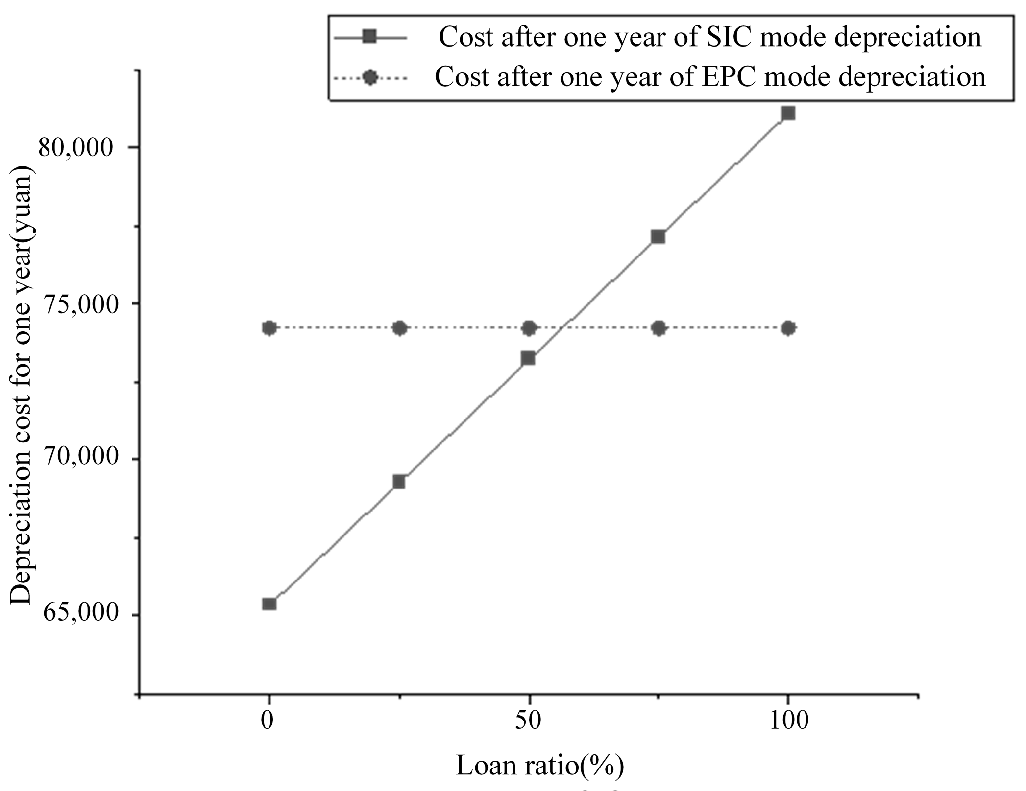
4.2.2. Comparison of Costs for Different Loan Ratios

The previous two cost comparison scenarios are based on the assumption that farmers’ construction funds are entirely sourced from loans. Different loan ratios influence the cost structure in the SIC model, which, in turn, impacts the decision-making process for selecting the project’s operational mode, as illustrated in Figure 2.

As illustrated in Figure 2, the one-year depreciation cost for the SIC model gradually increases as the loan ratio rises, reaching parity at a loan ratio of 56.39%. The EPC model becomes more cost-effective when the loan ratio surpasses this point, while the SIC model remains more advantageous when the loan ratio is below this threshold.

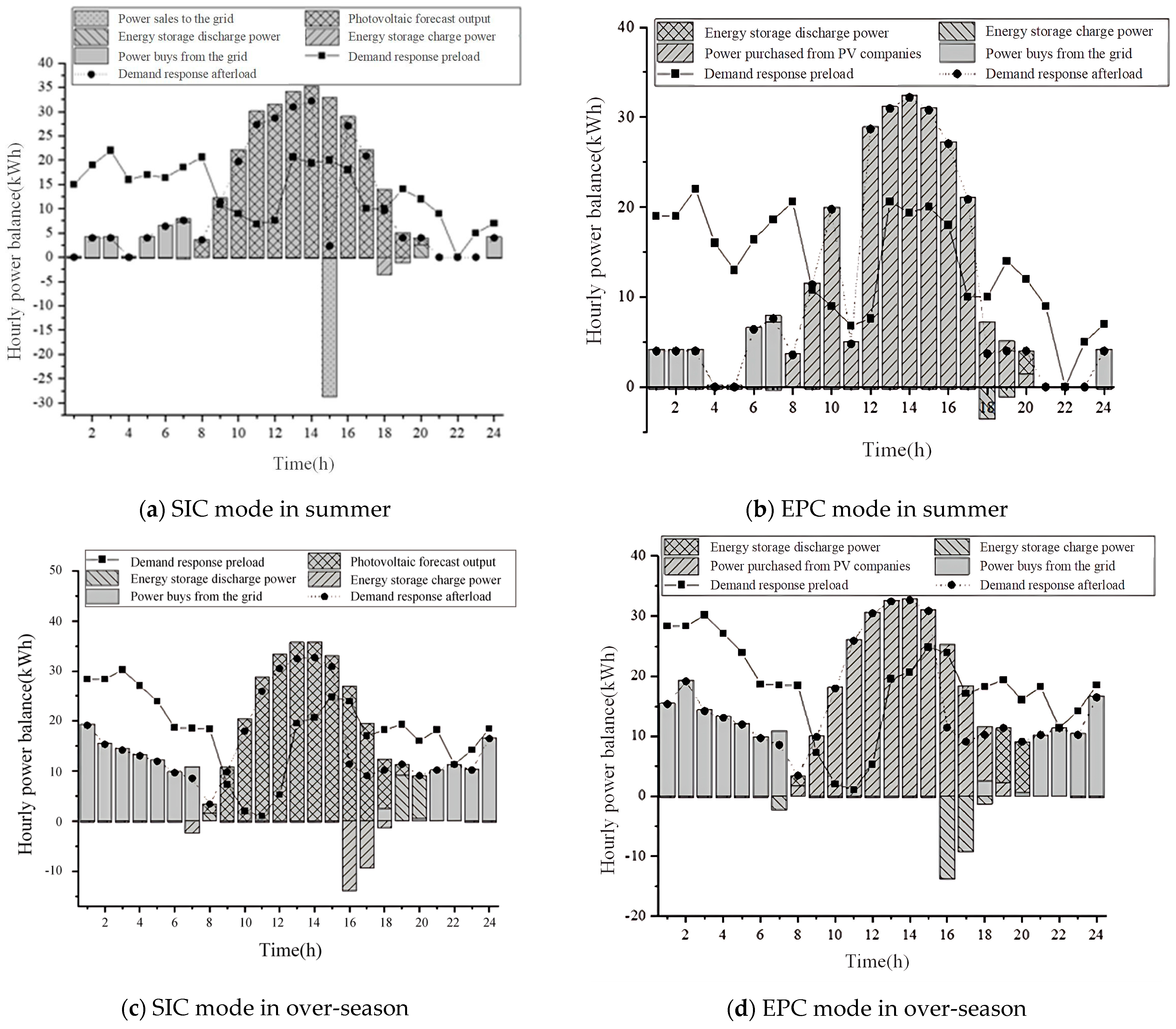
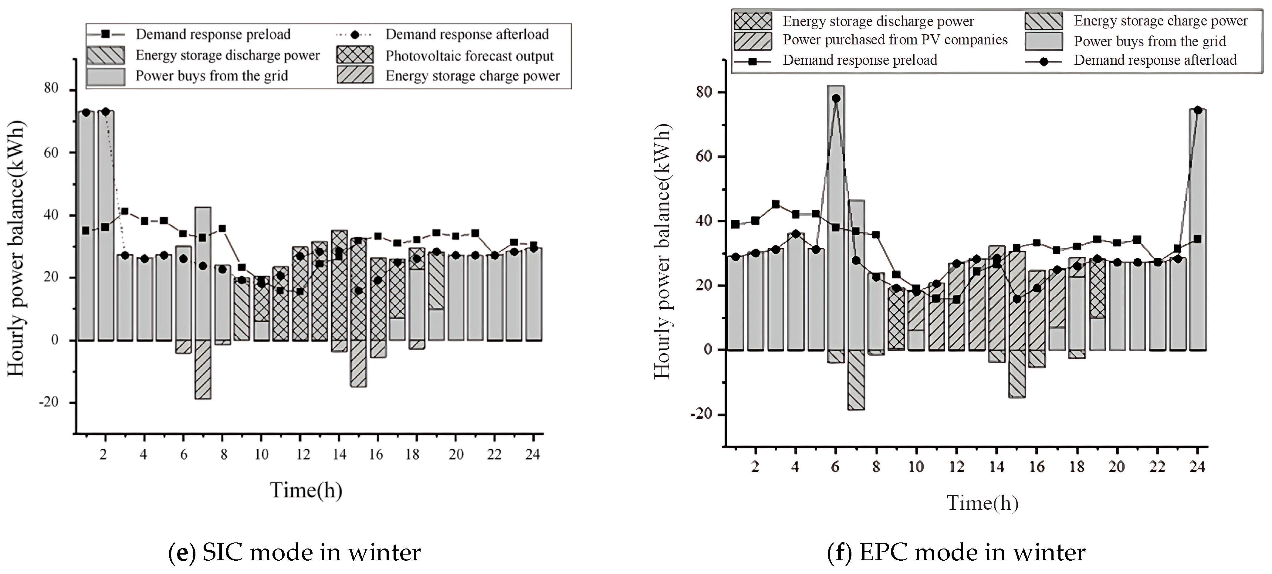
4.2.3. Optimization Analysis of Electricity Supply and Demand Strategies

The results of the optimization of the two modes of operation are shown in Figure 3.

(1) Summer Solstice Simulation Analysis

Figure 3a,b show that the highest PV output occurs between 9:00 to 17:00, with time-shiftable loads primarily concentrated in this period following demand response. The energy storage system is charged from 17:00 to 19:00 and discharged from 19:00 to 20:00. In the SIC mode, the PV output is generated on-site, and power is sold between 14:00 and 15:00. In the EPC mode, the PV output must be purchased from the PV enterprise. Due to identical tariffs during certain hours, multiple optimal solutions are available for demand response.

(2) Simulation analysis of over-seasonal days

Figure 3c,d indicate that in the SIC mode, there is no sale of electricity to the external grid for the entire period, suggesting that the PV output is insufficient to meet electricity demand. The charging and discharging strategies in both modes are generally similar, with load transfers executed according to the time-of-use tariff. Consequently, the load after partial transfer is significantly higher than it was before the transfer. The optimization results for both modes during the over-seasonal period are largely comparable, with multiple optimal solutions for demand response due to identical tariffs during certain periods.

(3) Winter Solstice Simulation Analysis

Figure 3e,f demonstrate that the optimal scheduling scenarios for both models are largely comparable. PV output decreases during the winter months while the energy demand from agricultural greenhouses rises. Consequently, it is essential to shift the time-sensitive load to the valley tariff period, leading to some post-transfer loads being significantly higher than their pre-transfer counterparts.

Figure 3 illustrates that the system must be paired with a specific energy storage system to fulfill the dispatch schedule, which can help reduce operating costs. The largest discharge power required is 18.67 kW.

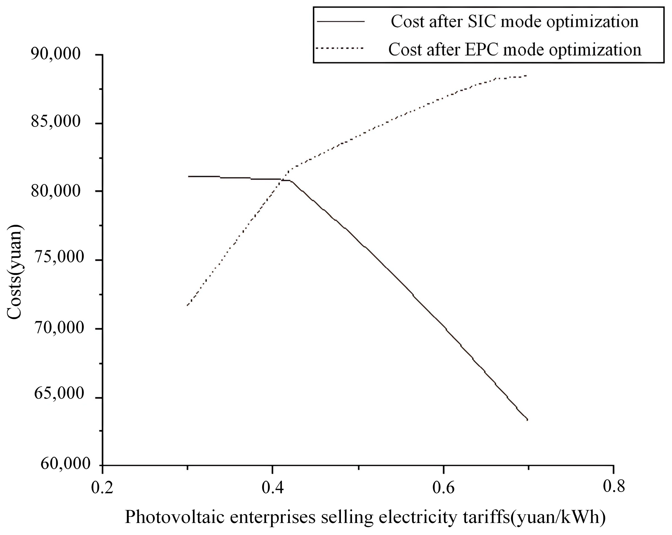
4.2.4. Sensitivity Analysis of Electricity Sales Tariffs

To ensure the profitability of the PV enterprise and enable farmers to benefit from preferential tariffs, the SIC mode sells electricity at the same price as the electricity purchased from the PV enterprise in the EPC mode. The optimal operating costs for the two modes are illustrated in Figure 4.

Figure 4 illustrates that when the price of electricity is less than or equal to 0.41 yuan/kWh, the EPC mode is more advantageous. Conversely, when the price exceeds 0.41 yuan/kWh, the SIC mode becomes preferable. In regions without large-scale PV enterprises, policy measures, including government subsidies, could be implemented to appropriately raise PV green electricity tariffs, thereby encouraging more farmers to invest in their own PV systems.

5. Conclusions

This study developed an optimal scheduling model for a PSAG, considering PV uncertainty and analyzing two operational modes. An agricultural greenhouse load model was established to accurately calculate the required energy load. As a case study, a specific agricultural greenhouse micro energy grid, which includes PV power generation units, energy storage systems, air-source heat pumps, refrigeration units, supplemental lighting, and other equipment, was optimally dispatched. A cost comparison under the two operational modes was conducted to determine the more favorable option. The simulation results indicate the following:

(1) In both modes, the derived optimal energy storage capacity remains consistent. It was determined that properly matching the energy storage system can significantly reduce the costs associated with the PSAG. This project necessitates a maximum energy storage capacity of 27.91 kWh and a maximum output power of 18.67 kW.

(2) Under the EPC mode, farmers purchase electricity from PV companies, which helps reduce the costs associated with PV agricultural greenhouses by installing PV systems on the greenhouses. The study indicates that the cost after one year of depreciation in the SIC mode is 81,083.69 yuan, whereas in the EPC mode, it is 74,216.22 yuan. Therefore, the EPC mode is more advantageous for farmers and is recommended for adoption.

(3) Different PV electricity sales tariffs impact farmers’ decisions regarding model selection. Policy subsidies can be utilized to modify the electricity prices associated with PV power generation, thereby influencing farmers’ choices between the two operational modes.

This study focuses primarily on the techno-economic optimization of the PSAG microgrid system, without comprehensively addressing the behavioral dynamics of end-users in energy participation mechanisms. Future work could integrate user-centric decision models to quantify the impact of incentive structures on farmers’ willingness to adopt EPC/SIC operational modes, thereby refining the dual-mode cost–benefit framework. Additionally, exploring multi-stakeholder game-theoretic approaches could optimize benefit distribution among investors, farmers, and grid operators, enhancing the scalability and social acceptability of PSAG deployments and fostering rural energy transitions.

References

1. Zhang, Z.; Pan, J.; Xiong, R.; Xiong, Z.; Chen, Y. Study on the Problems and Paths of Cleaner Rural Energy Consumption in Hubei Province under the Target of “Double Carbon”. Rural Econ. Sci.-Technol. 2023, 34, 227–230. [Google Scholar]
2. Li, W. Research on Capacity Allocation Optimization and Operation Scheduling of New Household Energy System in Rural Qinghai. Bachelor’s Thesis, Xi’an University of Architecture & Technology, Xi’an, China, 2023. [Google Scholar]
3. Cong, H.; Zhao, L.; Wang, J.; Yao, Z. Current situation and development demand analysis of rural energy in China. Trans. Chin. Soc. Agric. Eng. 2017, 33, 224–231. [Google Scholar]
4. Bardi, U.; Asmar, T.E.; Lavacchi, A. Turning electricity into food: The role of renewable energy in the future of agriculture. J. Clean. Prod. 2013, 53, 224–231. [Google Scholar] [CrossRef]
5. Yang, J.; Liu, Z. Development direction of distribution network in agricultural areas in China. Electr. Supply 2011, 28, 5–6+11. [Google Scholar]
6. Li, J.; Chen, S.; Wu, Y.; Wang, Q.; Liu, X.; Qi, L.; Lu, X.; Gao, L. How to make better use of intermittent and variable energy? A review of wind and photovoltaic power consumption in China. Renew. Sustain. Energy Rev. 2021, 137, 110626. [Google Scholar] [CrossRef]
7. Fernández, E.F.; Villar-Fernández, A.; Montes-Romero, J.; Ruiz-Torres, L.; Rodrigo, P.M.; Manzaneda, A.J.; Almonacid, F. Global energy assessment of the potential of photovoltaics for greenhouse farming. Appl. Energy 2022, 309, 118474. [Google Scholar] [CrossRef]
8. Yang, Y.; Feng, Y.; Wei, W.; Xie, P.; Chen, Y. Day-ahead-real-time cooperative scheduling of wind-fire-storage large bases based on consumption intervals. J. Shanghai Jiao Tong Univ. 2024, 1–24. [Google Scholar] [CrossRef]
9. Zhu, Y.; Yan, X.; Tong, Q. Optimal Design of Distributed Energy Systems in Rural Area of Developing Country: A Case Study of Guanzhong Area, China. IOP Conf. Ser. Earth Environ. Sci. 2018, 192, 012049. [Google Scholar] [CrossRef]
10. Yang, S.; Fang, J.; Zhang, Z.; Lv, S.; Lin, H.; Ju, L. Two-stage coordinated optimal dispatching model and benefit allocation strategy for rural new energy microgrid. Energy 2024, 292, 130274. [Google Scholar] [CrossRef]
11. Güven, A.F.; Mengi, O.Ö. Assessing metaheuristic algorithms in determining dimensions of hybrid energy systems for isolated rural environments: Exploring renewable energy systems with hydrogen storage features. J. Clean. Prod. 2023, 428, 139339. [Google Scholar] [CrossRef]
12. Kamal, M.; Ashraf, I.; Fernández, E. Optimal sizing of standalone rural microgrid for sustainable electrification with renewable energy resources. Sustain. Cities Soc. 2023, 88, 104298. [Google Scholar] [CrossRef]
13. Kamal, M.; Ashraf, I.; Fernández, E. Optimal renewable integrated rural energy planning for sustainable energy development. Sustain. Energy Technol. 2022, 53, 102581. [Google Scholar]
14. Suman, G.K.; Guerrero, J.M.; Roy, O.P. Optimisation of Solar/Wind/Bio-Generator/Diesel/Battery Based Microgrids for Rural Areas: A PSO-GWO Approach. Sustain. Cities Soc. 2021, 67, 102723. [Google Scholar] [CrossRef]
15. Chen, C.; Xing, J.; Li, Q.; Liu, S.; Ma, J.; Chen, J.; Han, L.; Qiu, W.; Lin, Z.; Yang, L. Wasserstein Distance-Based Distributionally Robust Optimal Scheduling in Rural Microgrid Considering the Coordinated Interaction among Source-Grid-Load-Storage. Energy Rep. 2021, 7, 60–66. [Google Scholar] [CrossRef]
16. Yadav, S.; Kumar, P.; Kumar, A. Hybrid Renewable Energy Systems Design and Techno-Economic Analysis for Isolated Rural Microgrid Using HOMER. Energy 2025, 327, 136442. [Google Scholar] [CrossRef]
17. Boccalatte, A.; Fossa, M.; Sacile, R. Modeling, design and construction of a zero-energy PV greenhouse for applications in mediterranean climates. Therm. Sci. Eng. Prog. 2021, 25, 101046. [Google Scholar] [CrossRef]
18. Azam, M.; Eltawil, M.; Amer, B. Thermal analysis of PV system and solar collector integrated with greenhouse dryer for drying tomatoes. Energy 2020, 212, 118764. [Google Scholar] [CrossRef]
19. Ghaffarpour, Z.; Fakhroleslam, M.; Amidpour, M. Calculation of Energy Consumption, Tomato Yield, and Electricity Generation in a PV-Integrated Greenhouse with Different Solar Panels Configuration. Renew. Energy 2024, 229, 120723. [Google Scholar] [CrossRef]
20. Haoyi, Y.; Yunfeng, W.; Xun, M.; Ming, L.; Fangling, F. An investigation on daylight in PV greenhouse for mushroom vertical cultivation in Kunming, China. Sol. Energy 2025, 291, 113414. [Google Scholar] [CrossRef]
21. Ghiasi, M.; Wang, Z.; Mehrandezh, M.; Paranjape, R. Enhancing Efficiency through Integration of Geothermal and Photovoltaic in Heating Systems of a Greenhouse for Sustainable Agriculture. Sustain. Cities Soc. 2025, 118, 106040. [Google Scholar] [CrossRef]
22. Wang, L.; Mao, Y.; Li, Z.; Yi, X.; Ma, Y.; Zhang, Y.; Li, M. Life Cycle Carbon Emission Intensity Assessment for Photovoltaic Greenhouses: A Case Study of Beijing City, China. Renew. Energy 2024, 230, 120775. [Google Scholar] [CrossRef]
23. Jamshidi, F.; Ghiasi, M.; Mehrandezh, M.; Wang, Z.; Paranjape, R. Optimizing Energy Consumption in Agricultural Greenhouses: A Smart Energy Management Approach. Smart Cities 2024, 7, 859–879. [Google Scholar] [CrossRef]
24. Zhu, Y.; Li, M.; Ma, X.; Wang, Y.; Li, G.; Zhang, Y.; Liu, Y.; Hassanien, R.H.E. Solar irradiance prediction with variable time lengths and multi-parameters in full climate conditions based on photovoltaic greenhouse. Energy Convers. Manag. 2024, 315, 118758. [Google Scholar] [CrossRef]
25. Attia, A.M.; Al Hanbali, A.; Saleh, H.H.; Alsawafy, O.G.; Ghaithan, A.M.; Mohammed, A. A Multi-Objective Optimization Model for Sizing Decisions of a Grid-Connected Photovoltaic System. Energy 2021, 229, 120730. [Google Scholar] [CrossRef]
26. Sun, T.; Jin, S.; Liu, G.; Hu, Y.; Qu, Y. Robust optimal allocation of photovoltaic town considering source-load uncertainty. Power Eng. Technol. 2023, 42, 42–51. [Google Scholar]
27. Cui, Y. Research on Home Energy Management Strategy Based on Robust Optimization. Bachelor’s Thesis, Shandong University, Jinan, China, 2023. [Google Scholar]
28. Wang, W.; Liu, F.; Yang, J.; Zheng, J.; Yang, Y.; Zhang, J. Optimal dispatch of micro-energy grid of photovoltaic smart agricultural greenhouse based on time-shiftable agricultural load. J. China Agric. Univ. 2018, 23, 160–168. [Google Scholar]
29. Wei, W.; Zhang, P.; Yao, M.; Xue, M.; Miao, J.; Liu, B.; Wang, F. Multi-Scope Electricity-Related Carbon Emissions Accounting: A Case Study of Shanghai. J. Clean. Prod. 2020, 252, 119789. [Google Scholar] [CrossRef]
Figure 1. Physical structure and energy flow diagram of a PSAG.
Processes 13 01622 g001
Figure 2. Costs under different loan ratios.
Processes 13 01622 g002
Figure 3. Operation optimization diagram of the two operating modes.
Processes 13 01622 g003aProcesses 13 01622 g003b
Figure 4. Electricity price sensitivity analysis diagram.
Processes 13 01622 g004