Abstract
In the domain of application of PN theory, the system deadlock problem of a flexible manufacturing system (FMS) is a thorny problem that needs to be solved urgently. All the research has the same objective of designing optimal controllers with maximal permissiveness and liveness. Plenty of the past literature used deadlock prevention as the main control strategy that is implemented by control places. However, these methods usually forbid undesirable system states from being reached, while reducing the system’s liveness. This study employed the resource flow graph (RFG)-based method to achieve a deadlock recovery policy that can maintain maximal permissiveness by adding control transitions (CTs). Also, we improved the current definition of RFG and developed a systematic approach for generating the corresponding RFG, which is based on flow mirroring pair (FMP) functions and the software Graphviz 12.2.1. Furthermore, this study proposed an automatic method that forms DOT script for generating Graphviz images, which is convincingly demonstrated in this study to enhance the execution efficiency and recognition of circular waiting situations.
1. Introduction
Flexible manufacturing systems (FMSs) [1,2,3,4,5] are a subject of significant interest within the field of industrial production. They are a highly adaptable and versatile production method, specifically designed to respond quickly to various production demands, volumes, and product designs. As a prominent type of resource allocation system (RAS), FMS provides better flexibility in product variety and contains automated tools such as robots and CNC machines, based on its resource-sharing framework. However, such sharing mechanisms can have a serious effect, potentially leading to the deadlock problem. Deadlock control has become a major area of interest within the field of FMS modeling.
Note that FMSs are a class of discrete event dynamic systems (DEDSs), and petri net (PN) theory [6,7,8,9,10,11,12,13,14] is used to analyze such systems in most research due to PN’s powerful analyzing ability for such problems. A typical sort of PN model called the system of simple sequential processes with resources (S3PR) net [3,13,15,16,17] is mainly used to simulate such concurrency systems. An S3PR net is a combination of simple sequential processes with resources (S2PR) nets and consists of various sequential processes, where deadlock usually occurs when certain resources are occupied.
There are mainly three strategies in the domain of deadlock control, including deadlock prevention [15,18,19,20,21,22], deadlock detection [23,24,25,26], and deadlock avoidance [27,28,29,30,31,32]. In the past literature, deadlock prevention has been used as the dominant control strategy, because it is able to form complicated constraints and nip deadlocks in the bud. These deadlock prevention policies are primarily achieved via analyzing the reachability graph and consequently result in much higher computational costs. Besides, this kind of strategy would lead to additional operational constraints on the original system and reduce the reachability and liveness of the entire system. This is contrary to the intent of FMS. In the authors’ view, it should not forbid the certain tendency of a system situation converting, merely because of these predictable errors, but try to preserve a more productive flexibility and the possibility of the state transforming.
According to literature surveying, the difficulty of computing and analyzing greatly depends on the decisions of the control strategy. The deadlock control issue has been proven to be an NP-complete problem [5] with an inherently high level of computational complexity. Thus, any control policy that can lower the difficulty of utilization or investigation should be considered as a valid optimization. Moreover, some of its properties are also regarded as symbolic indicators, such as permissiveness, liveness and structural complexity. By adopting different indicators, each control strategy will be the optimal choice based on the specific goal. Within this study and our previous ones, we emphasize the maintenance of the entire liveness and reachability of FMSs. The control strategy of deadlock recovery [33,34,35,36,37,38,39,40,41,42,43,44,45] seems to be a better choice than others with such objectives.
Since Huang et al. [44] firstly proposed the concept of control transition CT, there seems to be an opportunity to solve the problem of low reachability and low permissiveness of traditional deadlock control policies. Just as with the common transitions, CT is also able to change the current system marking, and this concept can be further expanded. In terms of RG, each transition is regarded as paths between markings, and CT is the specific human-designed pathway. Accordingly, Huang et al. [44] reported a deadlock recovery policy by creating CTs to keep the system running under deadlock states. However, under this approach, the system rarely achieved overall liveness, but it provided a new direction for the study of high permissiveness and liveness.
In research on deadlock control based on PN, two analysis tools, structural analysis (SA) [15,16,22,46,47,48,49,50] and reachability graph analysis (RGA) [51,52,53,54,55,56,57,58], were implemented for investigating the network’s properties. SA is used to remove deadlock-prone characteristics through specific substructures such as siphon, which appears mostly in early research. It thereby achieves the control objective of designing a deadlock-free net of FMS. Another, RGA, sets the initial marking as a starting point and uses computer-aided engineering (CAE) software for operating simulation until all reachable system states (markings) are found. Then, it analyzes the relationship between each state. The relative literature reported that it usually acquires the optimal controller through RGA with better permissiveness and performance, which is also the most widely adopted analysis tool.
Chen et al. [59] proposed a representative control policy by combining the integer linear programming problem (ILPP) and place invariant (PI) techniques. This method greatly reduces the control objects via a vector covering approach and meanwhile holds the original behavior. It finally computes the optimal controllers via an iterative pattern that can fully solve the deadlock problem and allows all legal markings to be reachable.
Pan [38] followed up on previous research on transition-based controllers by proposing a different research direction based on the original approach in [44]. The original CT synthesis approach is to analyze each deadlock marking individually and design a related CT to recover them. This method successfully explored the controller with the highest efficiency through comprehensive enumerating, named generating and comparing aiding matrix (GCAM), whose expected goal is similar to the control objective declared in [59] and is to design a controller applicable to the most deadlock markings. In our subsequent studies [33], the computational cost of a GCAM-based policy is further reduced by considering fewer items to compare.
Furthermore, we have tried many innovative directions in our previous works [36,60,61,62] for designing the most effective control policy, which is different from the existing ones. In [60], we developed a PI-based control policy by constructing an isomorphic model, which can solve the deadlock problem in S4PR nets. In [61], we successfully removed the system deadlocks with just one controller. These implies that our past works have actually solved potential issues in the domain of deadlock control.
Lu et al. [35] proposed a ground-breaking subnet structure called resource flow graph (RFG) for the particular characteristic known as circular waiting for deadlock. Note that the high degree FMSs consist of multiple working sequences, which are connected by sharing common resources. The cause of deadlock is that the occupied resource cannot be released due to the lack of the subsequent one, and also that these operations repeatedly request the resources held by each other, which is a so-called circular waiting situation. This method designs accurate CTs to re-arrange tokens by discovering all potential RFGs, and duly releases resources to revitalize the system. Elsayed et al. [34] further utilized such a method with S4PR nets and solved the system deadlocks as forecast, implying that the concept of RFG can be applied to general cases with the deadlock caused by circular waiting.
Our preceding study [45] proposed an improvement to the RFG-based deadlock recovery policy in [35], which decreased the number of controllers while providing the identical liveness. We also defined the circular structure within the RFG in more detail, which is named the hold and request circuits (HRCs). However, the RFG-based control policies described above have issues during execution that generate RFG in manual ways that may lead to unexpected errors.
This paper provides a new solution for accidental mistakes and much lower computational speed within human execution. The proposed method can define the RFG precisely and be completed in an automatic pattern. Three typical S3PR cases are introduced in this study to demonstrate the proposed method.
The rest of the article is organized in the following way. Section 2 gives an overview of the basic PN theory and deadlock recovery technique. Section 3 reviews the definition of RFG and develops a novel numerical generating method. Section 4 organizes the method as an entire algorithm. Section 5 utilizes the method with S3PR nets and discusses all RFG-based approaches in different perspectives. Section 6 gives a brief summary and critique of the findings.
2. Preliminaries
2.1. The Basics of Petri Net
A PN net is also named a place/transition net (P/T net), which is a tuple such that . The nonempty and disjoint sets and consist of places and transitions, respectively. indicates the flow relation and is the weighted value labeled on each arc. A marking is a row vector and used to describe the arrangement of tokens within a well-marked PN model, where is the initial marking. Note that a marking is also written as for simplification.
Considering any node , the prefix of is defined as , and its pre-set would be . Likewise, the postfix of the node is defined as , whose post-set would be . The firing (or activation) event of each transition is concerned with the marking of its prefix, i.e., is only enabled for firing at a marking if , which is denoted as ; or unable as . If the system would be transformed from marking into another one via firing , it is indicated as . A PN model is also presented as a matrix named the incidence matrix , which can be separated as the input incidence matrix and the output one such that .
Definition 1.
(Firing rule) Given a PN model . Let and be two reachable markings such that , while .
Moreover, an ordered sequence of transition is called the firing sequence such that . If can be reached from via firing the sequence of transition , where can be simplified as .
In research on PN modeling, an S3PR net is a typical class of PNs and is extensively used for simulating concurrency systems such as FMSs. An S3PR includes three types of places: the idle, operation and resource places, whose sets are denoted as , and , respectively. The idle place implies the capacity of raw materials for products, where each process contains only one idle place. The operation place is also named an activation place, which represents each step of the production processes. The resource place is set between certain operation places of various processes. The S3PR net is defined as follows:
Definition 2.
Given a S3PR net consisting of multiple processing subnets , which holds:
- is the set of idle places, where each of them is exclusive in the circuit it belongs to. For each , ;
- is the set of operation places and each element is marked as zero initially;
- is the set of resource places, where , , ;
- The sets , and are not empty sets with ;
- is the set of transitions.
A basic example of an S3PR net is presented in Figure 1. S3PR is short for a system of S2PR [3], such that an S3PR net consists of multiple S2PR processes by sharing resources, while such sharing behavior leads to deadlock problems due to over-requesting and competition. The related research aims to develop an optimal deadlock control policy, as in this paper. In the following sections, the proposed control policy is going to be constructed via a novel incidence matrix-based calculating technique.
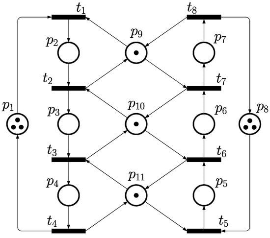
Figure 1.
A typical PN model of FMS that is adopted as Example 1 in this paper.
2.2. Reachability Graph Analysis
According to the firing rule above, each firing event transforms the system into a new state. All markings of a deadlock-free system are able to reach the initial marking from itself, and all reachable markings and the corresponding transforming paths (shown as arcs) are illustrated as the RG. By contrast, when the system is under a deadlock situation, there is no transition allowed to be activated. The RG can be classified as different areas according to the markings’ various properties, and the RG analysis discusses the subareas and their properties. Here, we give the related definitions as follows.
Definition 3.
(Reachable markings) Given an S3PR net and its PN model with the initial marking , the corresponding RG would be . Each reachable marking satisfies , such that . The set of is denoted as .
Definition 4.
(Legal markings) Let be the set of legal markings, where it holds that , , .
Definition 5.
(Deadlock markings) Let be the set of deadlock markings, where it holds that , , s.t. .
Definition 6.
(Quasi-deadlock markings) A marking is said to be a quasi-deadlock marking if it eventually reaches a deadlock but is not deadlocked yet. is the set of all quasi-deadlock markings that holds .
As a model’s scale and construction grows, the corresponding RG extends exponentially. It will be much harder to analyze different types of markings through manual classification. We are trying to develop a deadlock control strategy for models of various scale and construction. According to the firing rules above, each is able to transform the system into a new or existing marking. The transition-based supervisor is the extension of such a concept, which is used for recovering the reachability of deadlock markings. The RG analysis is also utilized on the proof of a partial deadlock.
2.3. Control Transition
Note that the shared parts in FMSs are the main cause of unexpected competition. In accordance with PN theory, all paths in RG are formed by activating each . However, there must exist some paths in RG that eventually point to deadlock markings in uncontrolled and deadlocked FMSs. To break from such a situation, it needs additional well-designed transitions for achieving the control objective, instead of just manually drawing intuitive paths. Our work seeks to develop an optimal deadlock recovery policy for designing efficient controllers.
RG-based analysis methods can identify the paths across different areas in RG to clarify the properties of all reachable markings. An initial objective of this research is to identify the type of marking and to verify the reachable paths in RG.
A previous study [44] proposed a transition-based controllers synthesis, which is also called a control transition (CT), in relevant areas by choosing two certain reachable markings as the terminals of the path. The details of CT, e.g., its input/output nodes and related weights, are obtained by simple matrix subtraction. Here, we give an overview of such a method.
Let be a PN model consisting of an uncontrolled S3PR net and the optimal controller set , where . is the set of all CTs that can recover all deadlocks, such that . According to the path generating synthesis of [44], in RG, the starting extremity of would be and the ending extremity would be . For two markings and , it is known that . Considering and as matrices, and the value of is calculated as follows:
where is indicated as for easy understanding in this manuscript, based on its property in RG. Via Equation (1), it is verified that is a matrix, just as in other regular transitions, but such a calculation is simple and inefficient. Here, we introduce a CT synthesis with higher efficiency in the following section.
3. Controller Synthesis
The sections above have shown that CT has a better performance than CP, including low computational complexity and much higher permissiveness. The CP-based control strategies using RG analysis usually calculate the controllers by iterative integer linear programming due to the NP-complete complexity and the optimization problem being subject to plenty of constraints. Thus, CP-based control policies imply the imposition of a large number of operating restrictions. The optimal solution of an integer linear programming problem is usually close to the limit and accordingly hard to compute, especially in deadlock-prone systems, which have high shareability and a complicated structure. Nevertheless, CT’s properties are a good remedy for these disadvantages.
Within the existing RG-based CT control policies, a CT is manually generated and able to form additional paths, which activates deadlocks and raises system liveness. Please note that a highly efficient CT can activate (recover) one or more deadlocks. Furthermore, the RFG-based recovery policies prevent the need for a shedload of calculations, such as the marking explosion problem in RG-based methods. This kind of methodology is regarded as the most efficient strategy in the domain of deadlock recovery in terms of its high liveness and exceedingly low computational complexity.
3.1. RFG-Based CT Synthesis
Lu et al. [35] proposed RFG-based CT synthesis, which can recover all deadlocks and solve the repeatedly requesting problem. Then, our previous study [45] improved the RFG-based method and successfully decreased the number of added CTs, achieving the same objective. This section gives a brief overview of such methods.
RFG is an extension of a PN model that is depicted by verifying the resource flows. Via an RFG of an S3PR net, one can know whether the resource is sent to certain processes or back to a resource container. That is, the resource flows can be separated into two types. Note that the resource flow is just an abstract notion for helping with conceptualization. According to the FMS definition, the resources usually imply robots or machines, which are occupied by operational processes and are not actually transported within a system. The RFG of the PN model can be constructed via the following definition.
Definition 7.
Let be the RFG of the net . and are the set of nodes and edges, respectively, and indicates the RFG’s state, which holds:
- The set is defined as , ;
- The set contains all nodes as each two terminals of , where ;
- is regarded as the partial marking of , which is usually the initial marking of the places in when considering the resource allocating condition at the beginning, i.e., ;
- An RFG contains at least one cycle structure , such that ; . Let , there must exist a path from to . is also an elementary cycle where all nodes are touched once at most.
The definition verifies the flow of resources and from which operation places they proceed. Besides, certain resources are alternately utilized across different production processes due to the sharing characteristic of FMS, which accordingly causes them to form a circular structure in RFG. Such a looping circuit implies a sequential relationship in occupying resources across different processes. Let be an operation place in RFG for example, where and indicates the resources before and after it, respectively. It must acquire the resource in to start the operation . Similarly, it has to acquire the resource in to close the operation and start the next one in the same process sequence. As aforementioned, the resource flow is merely an abstract concept and visualization based on RFG can help with understanding such ideas better. By verifying the resource flow situation, we aim to prevent the system from entering an unexpected deadlock state, which occurs when the essential resources of one certain operation process are sent to various processes. Such a circumstance is proven as follows.
Theorem 1.
Considering an operation place and two nearing nodes in RFG, the input (output) one implies the resource used in activating (ending) the operation.
Proof.
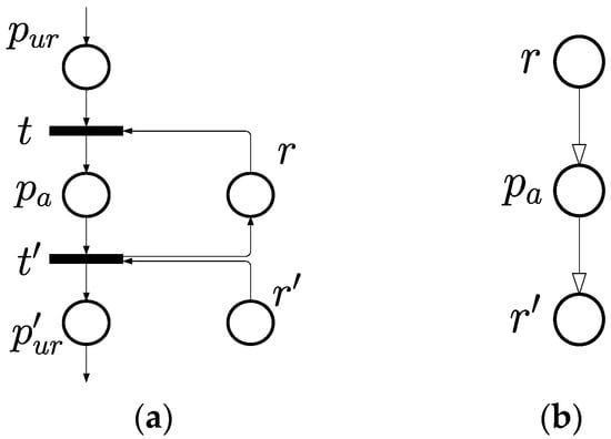
Considering a subnet of S3PR net as in Figure 2 for better understanding of the following proofs. Let be a node in RFG, as in Figure 2b, indicating an operation place which is unmarked in , such that . Suppose there exist two edges nearing , which are and and depicted as in RFG. With the definition of resource flow above, it needs the resource to begin operation , so as the operation that follows requires . Such an inference, based on the ordered relation of requesting, can be proven by the definition of transition firing in PN and the structural properties of the S3PR net. Let and be two transitions nearing in the PN model, such that , and , be the former/latter process of , respectively. Here we can further clarify the properties of and . For , the input nodes would be and , and the output node would be . Similarly, in terms of , , , , and . Then, it is accordingly known that when activating the operation . In addition, to end the operation , , . □
Figure 2.
A subnet of an S3PR net example: (a) the PN model; (b) the RFG form.
Theorem 2.
Partial deadlock occurs in an S3PR net when all resources belonging to a circuit are occupied at the same time, which eventually results in system deadlock.
Proof.
The definition of system deadlock is revealed in the section on PN basics. However, system deadlock is the eventual result of system operation. A control strategy based on the characteristic of deadlock marking is certain to make the system implement undesired redundant processes. In short, it can greatly increase control efficiency by analyzing the tendency of generating deadlock, e.g., partial deadlock, rather than of system deadlock itself. Thus, we define partial deadlock for verifying such a trend as follows, which has been proposed in [35]. Suppose there exist multiple shared resources between different operation sequences. Let be the set of these shared resources and be the set of sequences related to , where , , ; , . According to Definition 7, a resource flow circuit is obtained through and the related operation sequences, where , . It is clear that the subnet is deadlocked, when each resource place in is unmarked and there are no tokens in them. In terms of the whole S3PR net, such a situation is so-called partial deadlock. A partial deadlock marking makes these resources enter circular waiting due to the definition of RFG. Thus, a system with one or more partial deadlocks will eventually enter deadlock marking. □
Through defining the partial deadlock and resource flow circuit, the tendency of deadlock generating is clarified. Compared to the system deadlock-based control policies, the partial deadlock-based ones are much more efficient because there is no need to run redundant processes anymore. Conforming to the definition of RG, the system is initially under legal markings, and they become quasi-deadlock or deadlock markings after certain transitions are fired. Partial deadlock usually exists in legal or quasi-deadlock markings rather than deadlock ones. A partial deadlock-based control policy can recover the system much earlier than a system deadlock one can. The CT synthesis based on RFG for recovering a partial deadlock is given as follows.
Definition 8.
Let , be resource flow circuits in , such that , and corresponds to only one CT , where the pre dataset is and the post dataset is .
In order to break the circular waiting state in partial deadlock markings, the CT is designed to re-arrange the resources occupied by particular operations. The firing condition is set such that all the operation places are marked. Then, all these tokens will be sent to the original resource places after activating CT.
Theorem 3.
RFG-based CT is able to solve either system deadlock or partial deadlock markings with higher efficiency than an eventual deadlock state-based one.
Proof.
Let be a valid resource circuit and be the corresponding generated CT, where , . Let be the set of markings with partial deadlock and be the deadlock markings with partial deadlock , where . For clarifying the advantages of the RFG-based deadlock strategy in detail, it is necessary to introduce a real sequence in RG. Let be a certain reaching path in RG, where , , , i.e., all the markings in order after are with the partial deadlock such that . Since is going to fire when all nodes in are marked, i.e., under partial deadlock , will be enabled once the system enters . That is, those markings after would most likely never be reached, and the transitions to would not be fired if the partial deadlock situation is broken during . In addition, the rest of the unused resources in will not be wasted in the following steps, such that , . Then, the higher behavior of RFG-based CT is accordingly demonstrated. □
Via the definitions and proofs, the CT synthesis based on RFG has been proven with better behavior on deadlock control. When considering the control policy in general, however, building RFG is the only procedure that detects those feasible system components one-by-one and visualizes them manually. It is clearly hard to achieve the best control performance and such a strategy is prone to mistakes. Manual analysis has been validated as liable to make mistakes [63,64]. Also, it is difficult to deal with extremely large and complicated systems by the known RFG-based methods. A numerical calculation based on resource flow with higher efficiency and precision is proposed as follows.
3.2. Flow Mirroring Pair-Based CT Synthesis
The RFG-based CT synthesis mentioned above obviously suffers from disadvantages, such as the error due to human handling and higher time consumption, especially in the iterative cases. From the perspective of functionating, it is clear that discussing only the RFG’s definitions is not sufficient to establish a useful control policy. For preventing such issue, this study aims to overcome it by developing a numerical approach with less uncertainty.
By investigating the properties of RFG, the generating procedure seems able to be completed through an incidence matrix. Here, we gives an overview of the experimental process, which can also be illustrated as Figure 3.
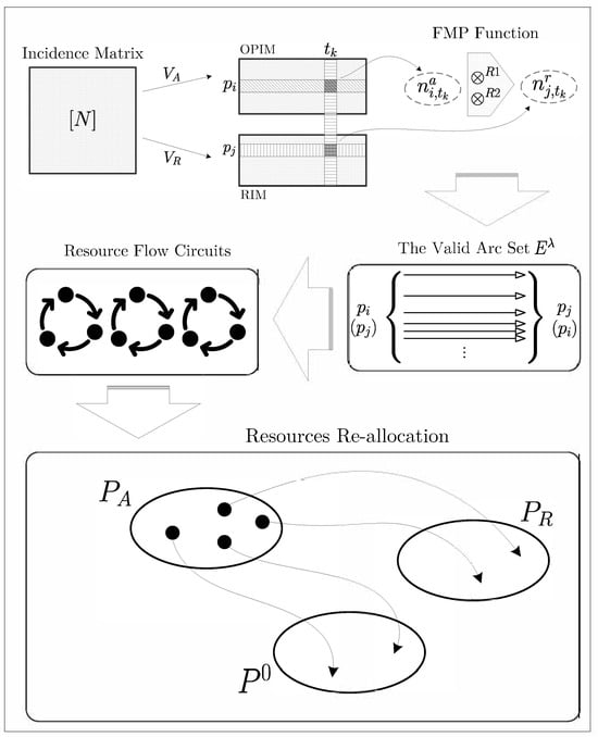
Figure 3.
Overview of transition-based deadlock recovery method via the RFG technique and FMP function.
- Build the incidence matrix via the input S3PR net;
- Separate it into two submatrices that represent operation and resource places;
- Do a comparison by each transition and pick all of the valid arc pairs up;
- Convert the arc pairs into the edges of the RFG;
- Output the RFG.
According to the basics of PN theory, a PN model can be presented as its incidence matrix, which also shows the resource flow well. The occurrence of system deadlocks is usually attributed to repeatedly requesting resources, which is caused by faulty system design. That is to say, it is easier to lead to circular waiting by placing multiple processes (especially the input arc of transitions) too close to the essential resource. And the incidence matrix helps clarify such resource requesting patterns. When considering each column of an incidence matrix, it shows all input/output arcs of every transition. In general, the operation place is regarded as the main cause of competition for resources in the previous literature. Thus, we only pick the operation and resource place as the control objects. The preprocessing is defined as follows.
Definition 9.
Given an incidence matrix of the PN model with the initial marking , let the Boolean form of be . There are three filters accordingly obtained as , and , where . Then, the submatrices are defined as and .
By the definition above, the incidence matrix is separated into two parts, including the operation incidence matrix (OPIM) and resource incidence matrix (RIM). The resource requesting event is related to these two submatrices. Also, the edges of the RFG can be classified as two types, the resource requesting and releasing, which have been proven in Theorem 1. One of the main objectives of this paper is to invent a novel method to obtain the optimal CTs without illustrating the RFG. The proposed numerical computation method can accurately finish the controller synthesis with no unexpected errors.
Axiom 1.
The input/output nodes of a valid transition of an S3PR net are known as the subnet of , implying the direction of the working process and the utilization of shared resources. Those arcs between the transition and resource place can be regarded as requesting or releasing events based on the corresponding input/output direction.
By Axiom 1, an arc pairing function is developed as follows to verify the arc types.
Definition 10.
Given two arcs and connecting to transition such that , the arc pairing function is used for arc type recognizing.
It is known that all the arc weights in an S3PR net are one. Thus, the possible value of each element in would be . The function has nine possible values in total. In terms of resource flow-based research, only two of them need to be considered, and the others would be ignored as zero. For better presentation, the predecessor and successor of one valid arc are represented as and , where .
Definition 11.
(Flow Mirroring Pairing Function) Given two nodes and nearing the same transition with valid connecting arcs, where the value of their counterpart would be nonzero, then the FMP function is defined as two types:
- R1-type is the arc pair with receiving the resource in and sending it to the operation for activating, such that . Note that the order of is thus opposite from .
- R2-type is the arc pair finishing the operation in and requesting the resource in for entering the next process, such that .
To compute the function , the OPIM and RIM need to be figured out at first. For extending it as the aspect of the entire matrix, we define the operator and such that and , where , . The entire equation is expanded as follows.
and so on as the R2-type FMP function’s computation. The equation above only considers the OPIM and RIM under the transition , i.e., finding out all valid arc pairs connecting to . All the valid arc pairs of R1-type and R2-type are presented as:
where , .
And the set of all valid nodes is defined as:
The entire RFG is then obtained by utilizing (3) and (4), such that .
For ease of understanding, here we introduce a simple net for application.
Example 1.
Considering the PN model in Figure 1 consisting of two process sequences. The initial state of this net is marked as .
This S3PR net is a typical and representative case in the domain of FMS and has been used in lots of research for developing various deadlock control strategies. Here, we construct the incidence matrix first, as shown as Equation (5) with the zero items omitted for easily reading. Let the Boolean form of be . Then, the three filters can be figured out by Definition 9, where , , . The submatrices of the operation and resource subnets are defined as below.
Through the two submatrices, the system of R1-type and R2-type FMP functions for all transitions is presented as follows, where , ,,,,,, , .
Via Equations (8) and (9), all the R1-type and R2-type arcs can be listed as Table 1. In this study, we use Graphviz [65,66] for RFG visualizing. The DOT script of the RFG of Example 1 is shown as Listing 1, and the RFG is shown as Figure 4, where the operation places are depicted as rectangles and the resource places as pentagons. Note that in the RFG of Graphviz form in this manuscript, the arcs of each circuit are drawn in the same color, and the arcs not appearing in any circuit are drawn as dashed arrows.

Table 1.
The set of all valid R1-type and R2-type arc pairs of Example 1.
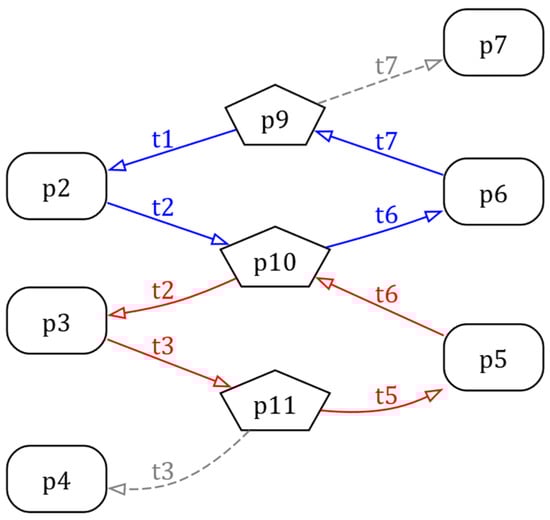
Figure 4.
The RFG of the PN model in Figure 1 depicted by Graphviz.
| Listing 1. The DOT script for the RFG visualization of Example 1. | |
| 1 | digraph RFG_FMS01{ |
| 2 | node [shape=box, style=rounded] p2 p3 p4 p5 p6 p7 |
| 3 | node [shape=pentagon, style=““] p9 p10 p11 |
| 4 | |
| 5 | p9 -> p2 [label=“t1”,color=blue,fontcolor=blue] |
| 6 | p2 -> p10 [label=“t2”,color=blue,fontcolor=blue] |
| 7 | p10 -> p6 [label=“t6”,color=blue,fontcolor=blue] |
| 8 | p6 -> p9 [label=“t7”,color=blue,fontcolor=blue] |
| 9 | p10 -> p3 [label=“t2”,color=red,fontcolor=red] |
| 10 | p3 -> p11 [label=“t3”,color=red,fontcolor=red] |
| 11 | p11 -> p5 [label=“t5”,color=red,fontcolor=red] |
| 12 | p5 -> p10 [label=“t6”,color=red,fontcolor=red] |
| 13 | p9 -> p7 [label=“t7”,style=dashed,color=gray,fontcolor=gray] |
| 14 | p11 -> p4 [label=“t3”,style=dashed,color=gray,fontcolor= gray] |
| 15 | } |
It is clear that there are a total of two circuits in Figure 4, including and . And the two related CTs are obtained as and . After the two CTs are added to the original model, the controlled system is checked as deadlock-free by simulating tool INA [67], which is shown as Figure 5.

Figure 5.
The controlled net of Figure 1 with two generated CTs, and .
4. Algorithm
This section synthesizes the previous methods and definitions into a systematic control policy, especially the procedure for generating the RFG. By utilizing such a deadlock recovery policy, the RFG will be built more accurately and quickly with no need to figure out the RG. The proposed method prevents human error and visualizes the situation immediately, which is believed to replace the former ones. The aforementioned theorems can be organized as the following Algorithm 1.
| Algorithm 1: The FMP-based RFG generating method and the valid CT set |
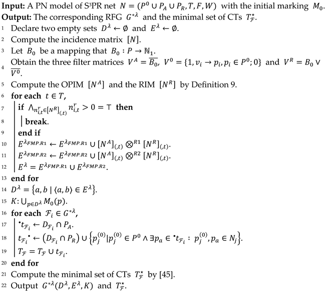 |
After completing the entire RFG, each circuit can be transformed into CT. Though these arc pairs are regarded as the edges of the RFG, we still can visualize it via another automatic way. As shown in Listing 1 and Figure 4, the RFG is converted into the DOT script and illustrated by the software Graphviz automatically. Here, we give the converting procedure from to the Graphviz image in Algorithm 2.
| Algorithm 2: Generating Graphviz script for RFG visualization. | |||
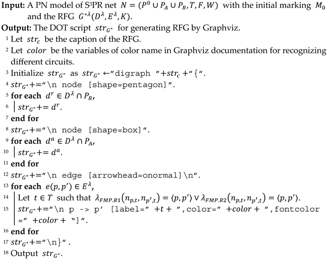 | |||
Through implementing the two proposed algorithms directly, the corresponding RFG can be easily and correctly illustrated. It is convincing that the proposed method provides a systematic solution for application and is able to prevent unforeseen mistakes.
5. Experimental Results
This section introduces two typical S3PR examples for demonstrating the proposed method. It is usually believed that the methods applicable to these two typical nets are able to be applied to most FMSs.
Example 2.
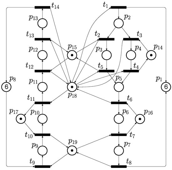
Consider the PN model shown as Figure 6, which has 19 places and 14 transitions in total. The set of places includes , and . The initial marking is set as .
Figure 6.
A typical PN model of FMS that is adopted as Example 2 in this paper.
Before the computation of RFG, it has to construct the incidence matrix, and the OPIM and RIM are accordingly obtained as follows.
All the valid arc pairs are shown as Table 2. Then, it can be converted into the DOT script shown as Listing 2 to form the visual RFG by Graphviz, which is presented as Figure 7.
Table 2.
The set of all valid R1-type and R2-type arcs of Example 2.
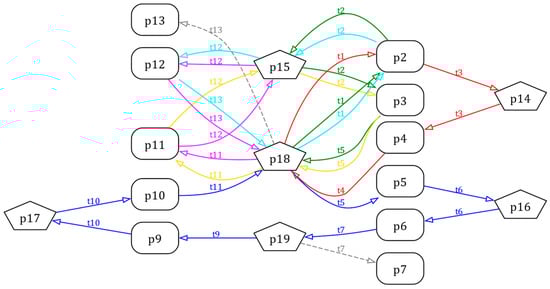
Figure 7.
The Graphviz form of the RFG of the PN model in Figure 6.
| Listing 2. The DOT script for the RFG visualization of Example 2. | |
| 1 | digraph RFG_FMS02{ |
| 2 | node [shape=pentagon] p14 p15 p16 p17 p18 p19 |
| 3 | node [shape=box] p2 p3 p4 p5 p6 p7 p9 p10 p11 p12 p13 |
| 4 | edge [arrowhead=onormal] |
| 5 | |
| 6 | p2 -> p14 [label=“t3”,color=red,fontcolor=red] |
| 7 | p14 -> p4 [label=“t3”,color=red,fontcolor=red] |
| 8 | p4 -> p18 [label=“t4”,color=red,fontcolor=red] |
| 9 | p18 -> p2 [label=“t1”,color=red,fontcolor=red] |
| 10 | p2 -> p15 [label=“t2”,color=green,fontcolor=green] |
| 11 | p15 -> p3 [label=“t2”,color=green,fontcolor=green] |
| 12 | p3 -> p18 [label=“t5”,color=green,fontcolor=green] |
| 13 | p18 -> p2 [label=“t1”,color=green,fontcolor=green] |
| 14 | p2 -> p15 [label=“t2”,color=cyan,fontcolor=cyan] |
| 15 | p15 -> p12 [label=“t12”,color=cyan,fontcolor=cyan] |
| 16 | p12 -> p18 [label=“t13”,color=cyan,fontcolor=cyan] |
| 17 | p18 -> p2 [label=“t1”,color=cyan,fontcolor=cyan] |
| 18 | p11 -> p15 [label=“t12”,color=gold,fontcolor=gold] |
| 19 | p15 -> p3 [label=“t2”,color=gold,fontcolor=gold] |
| 20 | p3 -> p18 [label=“t5”,color=gold,fontcolor=gold] |
| 21 | p18 -> p11 [label=“t11”,color=gold,fontcolor=gold] |
| 22 | p11 -> p15 [label=“t12”,color=fuchsia,fontcolor=fuchsia] |
| 23 | p15 -> p12 [label=“t12”,color=fuchsia,fontcolor=fuchsia] |
| 24 | p12 -> p18 [label=“t13”,color=fuchsia,fontcolor=fuchsia] |
| 25 | p18 -> p11 [label=“t11”,color=fuchsia,fontcolor=fuchsia] |
| 26 | p18 -> p5 [label=“t5”,color=blue,fontcolor=blue] |
| 27 | p5 -> p16 [label=“t6”,color=blue,fontcolor=blue] |
| 28 | p16 -> p6 [label=“t6”,color=blue,fontcolor=blue] |
| 29 | p6 -> p19 [label=“t7”,color=blue,fontcolor=blue] |
| 30 | p19 -> p9 [label=“t9”,color=blue,fontcolor=blue] |
| 31 | p9 -> p17 [label=“t10”,color=blue,fontcolor=blue] |
| 32 | p17 -> p10 [label=“t10”,color=blue,fontcolor=blue] |
| 33 | p10 -> p18 [label=“t11”,color=blue,fontcolor=blue] |
| 34 | p18 -> p13 [label=“t13”, color=gray,fontcolor=gray] |
| 35 | p19 -> p7 [label=“t7”, color=gray,fontcolor=gray] |
| 36 | } |
It is clear that there are six circuits in the RFG depicted in different colors, including , , , , , and . These circuits are converted into CTs by Definition 8, and the minimal set of CTs is computed by the method in [45], where . The contents of are shown as (13) to (16), such that the controlled system is checked deadlock-free after adding these CTs.
Next, we introduce another example for demonstration.
Example 3.
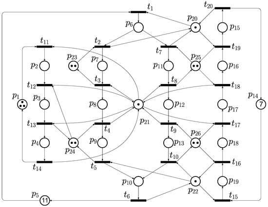
Consider the PN model shown as Figure 8, which has 26 places and 20 transitions in total. The set of places includes , and . The initial marking is set as .
Figure 8.
A typical PN model of FMS that is adopted as Example 3 in this paper.
The incidence matrix, OPIM, and RIM are calculated as Equations (17)–(19).
Then, all the valid arc pairs are generated via the FMP function and shown as Table 3, such that they are also regarded as the edges in the RFG for understanding the research concept. Then, these arc pairs are input to Algorithm 2 to generate the DOT script that is shown as Listing 3.
Table 3.
The set of all valid R1-type and R2-type arc pairs of Example 3.
| Listing 3. The DOT script for the RFG visualization of Example 3. | |
| 1 | digraph RFG_FMS03{ |
| 2 | node [shape=box,style=“rounded”] p2 p3 p4 p6 p7 p8 p9 p10 p11 p12 p13 p15 p16 p17 p18 p19 |
| 3 | node [shape=pentagon,style=““] p20 p21 p22 p23 p24 p25 p26 |
| 4 | edge [arrowhead=onormal] |
| 5 | |
| 6 | p22 -> p19 [label=“t15”,color=red,fontcolor=red] |
| 7 | p19 -> p26 [label=“t16”,color=red,fontcolor=red] |
| 8 | p26 -> p13 [label=“t9”,color=red,fontcolor=red] |
| 9 | p13 -> p22 [label=“t10”,color=red,fontcolor=red] |
| 10 | p12 -> p26 [label=“t9”,color=green,fontcolor=green] |
| 11 | p26 -> p18 [label=“t16”,color=green,fontcolor=green] |
| 12 | p18 -> p21 [label=“t17”,color=green,fontcolor=green] |
| 13 | p21 -> p12 [label=“t8”,color=green,fontcolor=green] |
| 14 | p3 -> p21 [label=“t13”,color=cyan,fontcolor=cyan] |
| 15 | p21 -> p8 [label=“t3”,color=cyan,fontcolor=cyan] |
| 16 | p8 -> p24 [label=“t4”,color=cyan,fontcolor=cyan] |
| 17 | p24 -> p3 [label=“t12”,color=cyan,fontcolor=cyan] |
| 18 | p3 -> p21 [label=“t13”,color=peru,fontcolor=peru] |
| 19 | p21 -> p2 [label=“t11”,color=peru,fontcolor=peru] |
| 20 | p2 -> p24 [label=“t12”,color=peru,fontcolor=peru] |
| 21 | p24 -> p3 [label=“t12”,color=peru,fontcolor=peru] |
| 22 | p11 -> p21 [label=“t8”,color=fuchsia,fontcolor=fuchsia] |
| 23 | p21 -> p17 [label=“t17”,color=fuchsia,fontcolor=fuchsia] |
| 24 | p17 -> p25 [label=“t18”,color=fuchsia,fontcolor=fuchsia] |
| 25 | p25 -> p11 [label=“t7”,color=fuchsia,fontcolor=fuchsia] |
| 26 | p9 -> p22 [label=“t5”,color=blue,fontcolor=blue] |
| 27 | p22 -> p19 [label=“t15”,color=blue,fontcolor=blue] |
| 28 | p19 -> p26 [label=“t16”,color=blue,fontcolor=blue] |
| 29 | p26 -> p18 [label=“t16”,color=blue,fontcolor=blue] |
| 30 | p18 -> p21 [label=“t17”,color=blue,fontcolor=blue] |
| 31 | p21 -> p2 [label=“t11”,color=blue,fontcolor=blue] |
| 32 | p2 -> p24 [label=“t12”,color=blue,fontcolor=blue] |
| 33 | p24 -> p9 [label=“t4”,color=blue,fontcolor=blue] |
| 34 | p9 -> p22 [label=“t5”,color=chartreuse,fontcolor=chartreuse] |
| 35 | p22 -> p19 [label=“t15”,color=chartreuse,fontcolor=chartreuse] |
| 36 | p19 -> p26 [label=“t16”,color=chartreuse,fontcolor=chartreuse] |
| 37 | p26 -> p18 [label=“t16”,color=chartreuse,fontcolor=chartreuse] |
| 38 | p18 -> p21 [label=“t17”,color=chartreuse,fontcolor=chartreuse] |
| 39 | p21 -> p8 [label=“t3”,color=chartreuse,fontcolor=chartreuse] |
| 40 | p8 -> p24 [label=“t4”,color=chartreuse,fontcolor=chartreuse] |
| 41 | p24 -> p9 [label=“t4”,color=chartreuse,fontcolor=chartreuse] |
| 42 | p7 -> p21 [label=“t3”,color=orangered,fontcolor=orangered] |
| 43 | p21 -> p17 [label=“t17”,color=orangered,fontcolor=orangered] |
| 44 | p17 -> p25 [label=“t18”,color=orangered,fontcolor=orangered] |
| 45 | p25 -> p16 [label=“t18”,color=orangered,fontcolor=orangered] |
| 46 | p16 -> p20 [label=“t19”,color=orangered,fontcolor=orangered] |
| 47 | p20 -> p6 [label=“t1”,color=orangered,fontcolor=orangered] |
| 48 | p6 -> p23 [label=“t2”,color=orangered,fontcolor=orangered] |
| 49 | p23 -> p7 [label=“t2”,color=orangered,fontcolor=orangered] |
| 50 | p20 -> p15 [label=“t19”,style=dashed,color=gray,fontcolor=gray] |
| 51 | p22 -> p10 [label=“t10”,style=dashed,color=gray,fontcolor=gray] |
| 52 | p21 -> p4 [label=“t13”,style=dashed,color=gray,fontcolor=gray] |
| 53 | } |
The RFG of the PN model of Example 3 is then presented as Figure 9 accordingly.
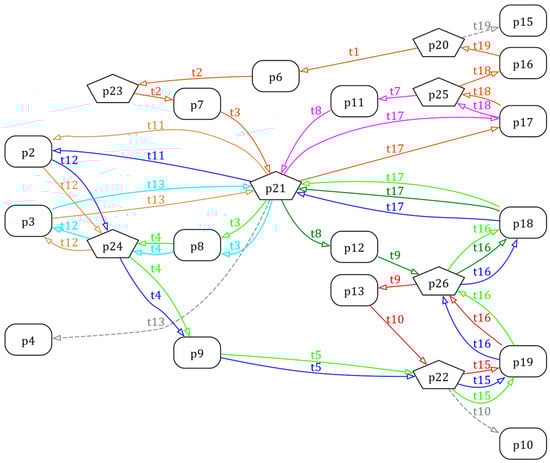
Figure 9.
The Graphviz form of the RFG of the PN model in Figure 8.
There are obviously nine circuits in the RFG, including , , , , , , , , . By the [45] method, the minimal set of CTs , where the contents are shown as follows:
Such that the controlled system with these eight CTs is checked as a deadlock-free system.
Through the two representative examples above, the proposed method is verified to have the ability to solve the deadlock problem in a more efficient control strategy. Here, we give the comparison of the RFG-based methods and the proposed one in various perspectives, which is shown as Table 4. And it is clear that the proposed method is implemented in an automatic way and does not suffer from manual errors. Furthermore, a comparison based on the experimental results of all transition-based methods of the Example 2 net is given as Table 5.
Table 4.
Comparison of the RFG-based methods and the proposed one.
Table 5.
Comparison of the transition-based deadlock recovery methods via experimental results on the PN Model of Example 2.
6. Conclusions
This study set out to design a transition-based deadlock recovery policy that is able to prevent the potential issue of human error and low efficiency and meanwhile maintain the original system performance. Based on the proofs presented in Section 3, the proposed RFG-based CT synthesis demonstrates equivalence in behavior to existing methods while exhibiting superior performance due to its enhanced numerical computation. Furthermore, the R1-type and R2-type FMP functions in this paper actually recognize the resource requesting tendency, which helps with organizing the following systematic control policy. In this study, we developed an innovative Graphviz-based algorithm for automatically depicting RFG merely through the generated data. This also facilitates a more precise and structured clarification of the resource flow associated with request and release processes, enhancing the overall comprehensibility and efficiency. Within the three examples in this manuscript, the proposed method is demonstrated to accomplish the same control objective with higher system liveness and computational efficiency. Despite its apparent results in this field, further work is required to establish the solutions with greater comprehensiveness.
Author Contributions
Conceptualization, W.-Y.C. and C.-Y.T.; methodology, C.-Y.T. and Y.-L.P.; software, K.-H.T.; validation, W.-Y.C. and K.-H.T.; formal analysis, W.-Y.C.; investigation, W.-Y.C. and C.-Y.T.; resources, Y.-L.P.; data curation, K.-H.T. and Y.-L.P.; writing—original draft preparation, W.-Y.C. and C.-Y.T.; writing—review and editing, C.-Y.T. and Y.-L.P.; visualization, C.-Y.T.; supervision, K.-H.T. and Y.-L.P.; project administration, Y.-L.P. All authors have read and agreed to the published version of the manuscript.
Funding
This research received no external funding.
Data Availability Statement
The data presented in this study are available in the article.
Conflicts of Interest
The authors declare no conflicts of interest.
References
- Javaid, M.; Haleem, A.; Singh, R.P.; Suman, R. Enabling Flexible Manufacturing System (FMS) through the Applications of Industry 4.0 Technologies. Internet Things Cyber-Phys. Phys. Syst. 2022, 2, 49–62. [Google Scholar] [CrossRef]
- Manu, G.; Vijay Kumar, M.; Nagesh, H.; Jagadeesh, D.; Gowtham, M.B. Flexible Manufacturing Systems (FMS), A Review. Int. J. Mech. Prod. Eng. Res. Dev. 2018, 8, 323–336. [Google Scholar] [CrossRef]
- Ezpeleta, J.; Colom, J.M.; Martinez, J. A Petri Net Based Deadlock Prevention Policy for Flexible Manufacturing Systems. IEEE Trans. Robot. Automat. 1995, 11, 173–184. [Google Scholar] [CrossRef]
- Banaszak, Z.A.; Krogh, B.H. Deadlock Avoidance in Flexible Manufacturing Systems with Concurrently Competing Process Flows. IEEE Trans. Robot. Automat. 1990, 6, 724–734. [Google Scholar] [CrossRef]
- Liu, G. Complexity of the Deadlock Problem for Petri Nets Modeling Resource Allocation Systems. Inf. Sci. 2016, 363, 190–197. [Google Scholar] [CrossRef]
- Murata, T. Petri Nets: Properties, Analysis and Applications. Proc. IEEE 1989, 77, 541–580. [Google Scholar] [CrossRef]
- Reisig, W. Petri Nets; Springer: Berlin/Heidelberg, Germany, 1985; ISBN 978-3-642-69970-2. [Google Scholar]
- Zhou, M.; Venkatesh, K. Modeling, Simulation, and Control of Flexible Manufacturing Systems: A Petri Net Approach; World Scientific: Singapore, 1999; ISBN 978-981-02-3029-6. [Google Scholar]
- Liu, G. Petri Nets: Theoretical Models and Analysis Methods for Concurrent Systems; Springer Nature: Singapore, 2022; ISBN 978-981-19-6308-7. [Google Scholar]
- Kaid, H.; Al-Ahmari, A.; Alqahtani, K.N.; Dabwan, A.; Nasr, M.M.; Alhaag, M.H. An Internet-of-Things Based on ILPP, Petri Nets, and Artificial Neural Networks for Controlling Tool Failures in Flexible Manufacturing Systems Under Complex Operational Conditions. IEEE Access 2025, 13, 37035–37050. [Google Scholar] [CrossRef]
- Reisig, W. Understanding Petri Nets: Modeling Techniques, Analysis Methods, Case Studies; Springer: Berlin/Heidelberg, Germany, 2013; ISBN 978-3-642-33277-7. [Google Scholar]
- Barylska, K.; Best, E.; Schlachter, U.; Spreckels, V. Properties of Plain, Pure, and Safe Petri Nets. In Transactions on Petri Nets and Other Models of Concurrency XII; Koutny, M., Kleijn, J., Penczek, W., Eds.; Lecture Notes in Computer Science; Springer: Berlin/Heidelberg, Germany, 2017; Volume 10470, pp. 1–18. ISBN 978-3-662-55861-4. [Google Scholar]
- Huang, B.; Zhou, M.; Lu, X.S.; Abusorrah, A. Scheduling of Resource Allocation Systems with Timed Petri Nets: A Survey. ACM Comput. Surv. 2023, 55, 1–27. [Google Scholar] [CrossRef]
- Yamalidou, K.; Moody, J.; Lemmon, M.; Antsaklis, P. Feedback Control of Petri Nets Based on Place Invariants. Automatica 1996, 32, 15–28. [Google Scholar] [CrossRef]
- Guo, X.; Wang, S.; You, D.; Li, Z.; Jiang, X. A Siphon-Based Deadlock Prevention Strategy for S3PR. IEEE Access 2019, 7, 86863–86873. [Google Scholar] [CrossRef]
- Abdul-Hussin, M.H. On Structural Conditions of S3PR Based Siphons to Prevent Deadlocks in Manufacturing Systems. Int. J. Simul. Syst. Sci. Technol. 2016, 17, 32.1–32.8. [Google Scholar] [CrossRef]
- Feng, Y.; Xing, K.; Zhou, M.; Chen, H.; Tian, F. Polynomial-Complexity Robust Deadlock Controllers for a Class of Automated Manufacturing Systems with Unreliable Resources Using Petri Nets. Inf. Sci. 2020, 533, 181–199. [Google Scholar] [CrossRef]
- Abdallah, I.B.; ElMaraghy, H.A. Deadlock Prevention and Avoidance in FMS: A Petri Net Based Approach. Int. J. Adv. Manuf. Technol. 1998, 14, 704–715. [Google Scholar] [CrossRef]
- Li, Z.; Zhao, M. On Controllability of Dependent Siphons for Deadlock Prevention in Generalized Petri Nets. IEEE Trans. Syst. Man Cybern. Part A 2008, 38, 369–384. [Google Scholar] [CrossRef]
- Chen, Y.; Li, Z. On Structural Minimality of Optimal Supervisors for Flexible Manufacturing Systems. Automatica 2012, 48, 2647–2656. [Google Scholar] [CrossRef]
- Chen, Y.; Li, Z.; Barkaoui, K.; Giua, A. On the Enforcement of a Class of Nonlinear Constraints on Petri Nets. Automatica 2015, 55, 116–124. [Google Scholar] [CrossRef]
- Zhuang, Q.; Dai, W.; Wang, S.; Du, J.; Tian, Q. An MIP-Based Deadlock Prevention Policy for Siphon Control. IEEE Access 2019, 7, 153782–153790. [Google Scholar] [CrossRef]
- Du, N.; Hu, H. Robust Deadlock Detection and Control of Automated Manufacturing Systems With Multiple Unreliable Resources Using Petri Nets. IEEE Trans. Automat. Sci. Eng. 2021, 18, 1790–1802. [Google Scholar] [CrossRef]
- Du, Y.; Gu, N.; Zhou, X. Accelerating Reachability Analysis on Petri Net for Mutual Exclusion-Based Deadlock Detection. IEICE Trans. Inf. Syst. 2016, 99, 2978–2985. [Google Scholar] [CrossRef]
- Zhou, M. (Ed.) Deadlock Resolution in Computer-Integrated Systems; Dekker: IJzendoorn, Netherlands; CRC Press: New York, NY, USA, 2005; ISBN 978-0-8247-5368-9. [Google Scholar]
- Tat Leung, Y.; Sheen, G.-J. Resolving Deadlocks in Flexible Manufacturing Cells. J. Manuf. Syst. 1993, 12, 291–304. [Google Scholar] [CrossRef]
- Xing, K.; Zhou, M.C.; Liu, H.; Tian, F. Optimal Petri-Net-Based Polynomial-Complexity Deadlock-Avoidance Policies for Automated Manufacturing Systems. IEEE Trans. Syst. Man Cybern. Part A 2009, 39, 188–199. [Google Scholar] [CrossRef]
- Wu, N.; Zhou, M.; Li, Z. Resource-Oriented Petri Net for Deadlock Avoidance in Flexible Assembly Systems. IEEE Trans. Syst. Man Cybern. Part A 2008, 38, 56–69. [Google Scholar] [CrossRef]
- Hsieh, F.-S. Fault-Tolerant Deadlock Avoidance Algorithm for Assembly Processes. IEEE Trans. Syst. Man Cybern. Part A 2004, 34, 65–79. [Google Scholar] [CrossRef]
- Ezpeleta, J.; Recalde, L. A Deadlock Avoidance Approach for Nonsequential Resource Allocation Systems. IEEE Trans. Syst. Man Cybern. Part A 2004, 34, 93–101. [Google Scholar] [CrossRef]
- Park, J.; Reveliotis, S.A. Deadlock Avoidance in Sequential Resource Allocation Systems with Multiple Resource Acquisitions and Flexible Routings. IEEE Trans. Automat. Contr. 2001, 46, 1572–1583. [Google Scholar] [CrossRef]
- Xing, K.-Y.; Hu, B.-S.; Chen, H.-X. Deadlock Avoidance Policy for Petri-Net Modeling of Flexible Manufacturing Systems with Shared Resources. IEEE Trans. Automat. Contr. 1996, 41, 289–295. [Google Scholar] [CrossRef]
- Pan, Y.-L.; Tseng, C.-Y.; Chen, J.-C. Enhancement of Computational Efficiency for Deadlock Recovery of Flexible Manufacturing Systems Using Improved Generating and Comparing Aiding Matrix Algorithms. Processes 2023, 11, 3026. [Google Scholar] [CrossRef]
- Elsayed, M.S.; Kefi, K.; Li, Z. An Optimal Transition-Based Recovery Policy for Controlling Deadlock Within Flexible Manufacturing Systems Using Graph Technique. IEEE Access 2023, 11, 51723–51739. [Google Scholar] [CrossRef]
- Lu, Y.; Chen, Y.; Li, Z.; Wu, N. An Efficient Method of Deadlock Detection and Recovery for Flexible Manufacturing Systems by Resource Flow Graphs. IEEE Trans. Automat. Sci. Eng. 2022, 19, 1707–1718. [Google Scholar] [CrossRef]
- Row, T.-C.; Pan, Y.-L. An Optimal Deadlock Recovery Algorithm for Special and Complex Flexible Manufacturing Systems-S4PR. IEEE Access 2021, 9, 111083–111094. [Google Scholar] [CrossRef]
- Pan, Y.-L.; Tai, C.-W.; Tseng, C.-Y.; Huang, J.-C. Enhancement of Computational Efficiency in Seeking Liveness-Enforcing Supervisors for Advanced Flexible Manufacturing Systems with Deadlock States. Appl. Sci. 2020, 10, 2620. [Google Scholar] [CrossRef]
- Pan, Y.-L. One Computational Innovation Transition-Based Recovery Policy for Flexible Manufacturing Systems Using Petri Nets. Appl. Sci. 2020, 10, 2332. [Google Scholar] [CrossRef]
- Dong, Y.; Chen, Y.; Li, S.; El-Meligy, M.A.; Sharaf, M. An Efficient Deadlock Recovery Policy for Flexible Manufacturing Systems Modeled With Petri Nets. IEEE Access 2019, 7, 11785–11795. [Google Scholar] [CrossRef]
- Row, T.-C.; Pan, Y.-L. Maximally Permissive Deadlock Prevention Policies for Flexible Manufacturing Systems Using Control Transition. Adv. Mech. Eng. 2018, 10, 168781401878740. [Google Scholar] [CrossRef]
- Bashir, M.; Liu, D.; Uzam, M.; Wu, N.; Al-Ahmari, A.; Li, Z. Optimal Enforcement of Liveness to Flexible Manufacturing Systems Modeled with Petri Nets via Transition-Based Controllers. Adv. Mech. Eng. 2018, 10, 168781401775070. [Google Scholar] [CrossRef]
- Chen, Y.; Li, Z.; Al-Ahmari, A.; Wu, N.; Qu, T. Deadlock Recovery for Flexible Manufacturing Systems Modeled with Petri Nets. Inf. Sci. 2017, 381, 290–303. [Google Scholar] [CrossRef]
- Zhang, X.; Uzam, M. Transition-Based Deadlock Control Policy Using Reachability Graph for Flexible Manufacturing Systems. Adv. Mech. Eng. 2016, 8, 168781401663150. [Google Scholar] [CrossRef]
- Huang, Y.-S.; Pan, Y.-L.; Su, P.-J. Transition-Based Deadlock Detection and Recovery Policy for FMSs Using Graph Technique. ACM Trans. Embed. Comput. Syst. 2013, 12, 1–13. [Google Scholar] [CrossRef]
- Tseng, C.-Y.; Chen, J.-C.; Pan, Y.-L. An Improved Deadlock Recovery Policy of Flexible Manufacturing Systems Based on Resource Flow Graphs. IEEE Access 2024, 12, 65202–65212. [Google Scholar] [CrossRef]
- Piroddi, L.; Cordone, R.; Fumagalli, I. Selective Siphon Control for Deadlock Prevention in Petri Nets. IEEE Trans. Syst. Man Cybern. Part A 2008, 38, 1337–1348. [Google Scholar] [CrossRef]
- Liu, D.; Li, Z.; Zhou, M. Hybrid Liveness-Enforcing Policy for Generalized Petri Net Models of Flexible Manufacturing Systems. IEEE Trans. Syst. Man Cybern Syst. 2013, 43, 85–97. [Google Scholar] [CrossRef]
- Lin, R.; Yu, Z.; Shi, X.; Dong, L.; Nasr, E.A. On Multi-Step Look-Ahead Deadlock Prediction for Automated Manufacturing Systems Based on Petri Nets. IEEE Access 2020, 8, 170421–170432. [Google Scholar] [CrossRef]
- Li, Z.; Zhou, M. Elementary Siphons of Petri Nets and Their Application to Deadlock Prevention in Flexible Manufacturing Systems. IEEE Trans. Syst. Man Cybern. Part A 2004, 34, 38–51. [Google Scholar] [CrossRef]
- Wang, S.; Duo, W.; Guo, X.; Jiang, X.; You, D.; Barkaoui, K.; Zhou, M. Computation of an Emptiable Minimal Siphon in a Subclass of Petri Nets Using Mixed-Integer Programming. IEEE/CAA J. Autom. Sinica 2021, 8, 219–226. [Google Scholar] [CrossRef]
- Shaoyong, L.; Chunrun, Z. A Deadlock Control Algorithm Using Control Transitions for Flexible Manufacturing Systems Modelling with Petri Nets. Int. J. Syst. Sci. 2020, 51, 771–785. [Google Scholar] [CrossRef]
- Hu, M.; Yang, S.; Chen, Y. Partial Reachability Graph Analysis of Petri Nets for Flexible Manufacturing Systems. IEEE Access 2020, 8, 227925–227935. [Google Scholar] [CrossRef]
- Zhuang, Q.; Dai, W.; Wang, S.; Ning, F. Deadlock Prevention Policy for S4 PR Nets Based on Siphon. IEEE Access 2018, 6, 50648–50658. [Google Scholar] [CrossRef]
- Gelen, G.; Uzam, M.; Li, Z. A New Method for the Redundancy Analysis of Petri Net-Based Liveness Enforcing Supervisors. Trans. Inst. Meas. Control. 2017, 39, 763–780. [Google Scholar] [CrossRef]
- Chao, D.Y.; Chen, J.-T.; Yu, F. A Novel Liveness Condition for S3PGR2. Trans. Inst. Meas. Control. 2013, 35, 131–137. [Google Scholar] [CrossRef]
- Uzam, M.; Zhou, M. An Iterative Synthesis Approach to Petri Net-Based Deadlock Prevention Policy for Flexible Manufacturing Systems. IEEE Trans. Syst. Man Cybern. Part A 2007, 37, 362–371. [Google Scholar] [CrossRef]
- Uzam, M.; Zhou, M.C. An Improved Iterative Synthesis Method for Liveness Enforcing Supervisors of Flexible Manufacturing Systems. Int. J. Prod. Res. 2006, 44, 1987–2030. [Google Scholar] [CrossRef]
- Ghaffari, A.; Rezg, N.; Xie, X. Design of a Live and Maximally Permissive Petri Net Controller Using the Theory of Regions. IEEE Trans. Robot. Automat. 2003, 19, 137–142. [Google Scholar] [CrossRef]
- Chen, Y.; Li, Z.; Zhou, M. Behaviorally Optimal and Structurally Simple Liveness-Enforcing Supervisors of Flexible Manufacturing Systems. IEEE Trans. Syst. Man Cybern. Part A 2012, 42, 615–629. [Google Scholar] [CrossRef]
- Row, T.-C.; Tseng, C.-Y.; Pan, Y.-L. Universal Single Controller for Solving Deadlock Problems of Flexible Manufacturing Systems. IEEE Access 2024, 12, 191907–191920. [Google Scholar] [CrossRef]
- Row, T.-C.; Pan, Y.-L. Incomparable Single Controller for Solving Deadlock Problems of Flexible Manufacturing Systems. IEEE Access 2023, 11, 45270–45278. [Google Scholar] [CrossRef]
- Row, T.-C.; Syu, W.-M.; Pan, Y.-L.; Wang, C.-C. One Novel and Optimal Deadlock Recovery Policy for Flexible Manufacturing Systems Using Iterative Control Transitions Strategy. Math. Probl. Eng. 2019, 2019, 4847072. [Google Scholar] [CrossRef]
- Sturdee, M. A Step Toward Formalising Visual Data Analysis Practices in Human Computer Interaction. Interact. Comput. 2025, 1–14. [Google Scholar] [CrossRef]
- Bajpai, A.; Yadav, S.; Nagwani, N.K. An Extensive Bibliometric Analysis of Artificial Intelligence Techniques from 2013 to 2023. J. Supercomput. 2025, 81, 540. [Google Scholar] [CrossRef]
- Ellson, J.; Gansner, E.R.; Koutsofios, E.; North, S.C.; Woodhull, G. Graphviz and Dynagraph—Static and Dynamic Graph Drawing Tools. In Graph Drawing Software; Jünger, M., Mutzel, P., Eds.; Mathematics and Visualization; Springer: Berlin/Heidelberg, Germany, 2004; pp. 127–148. ISBN 978-3-642-62214-4. [Google Scholar]
- Ellson, J.; Gansner, E.; Koutsofios, L.; North, S.C.; Woodhull, G. Graphviz—Open Source Graph Drawing Tools. In Graph Drawing; Mutzel, P., Jünger, M., Leipert, S., Eds.; Lecture Notes in Computer Science; Springer: Berlin/Heidelberg, Germany, 2002; Volume 2265, pp. 483–484. ISBN 978-3-540-43309-5. [Google Scholar]
- INA Integrated Net Analyzer Version 2.2. Available online: https://www2.informatik.hu-berlin.de/~starke/ina.html (accessed on 24 April 2025).
Disclaimer/Publisher’s Note: The statements, opinions and data contained in all publications are solely those of the individual author(s) and contributor(s) and not of MDPI and/or the editor(s). MDPI and/or the editor(s) disclaim responsibility for any injury to people or property resulting from any ideas, methods, instructions or products referred to in the content. |
© 2025 by the authors. Licensee MDPI, Basel, Switzerland. This article is an open access article distributed under the terms and conditions of the Creative Commons Attribution (CC BY) license (https://creativecommons.org/licenses/by/4.0/).