
Mathematical Modeling of Friction Reduction in Drilling Long Horizontal Wells Using Smooth Catenary Well Trajectories


Abstract
1. Introduction
2. Smooth Catenary Trajectory Design Procedure
- (1)
- Design the horizontal/slant wellbore length based on the well productivity requirement.
- (2)
- Design the length of the catenary section by specifying and .
- (3)
- Numerically solve for a-value from the following equation:
- (4)
- Calculate the radius of curvature (Rtop) and inclination angle (θtop) at the top end of the catenary section using the following equations:
- (5)
- Calculate the vertical displacement of the arc section above the catenary section using the radius of curvature at the top-end of the catenary section, i.e.,
- (6)
- Determine the KOP by
- (7)
- Calculate the vertical and horizontal coordinates in the arc section using the following inclination angle build rate expressed bywhere B is inclination angle build rate in degrees per unit length of arc.
- (8)
- Calculate the vertical and horizontal coordinates in the catenary section using the following inclination angle equation:
- (9)
- Calculate the vertical and horizontal coordinates in the horizontal/slant section based on the final inclination angle.
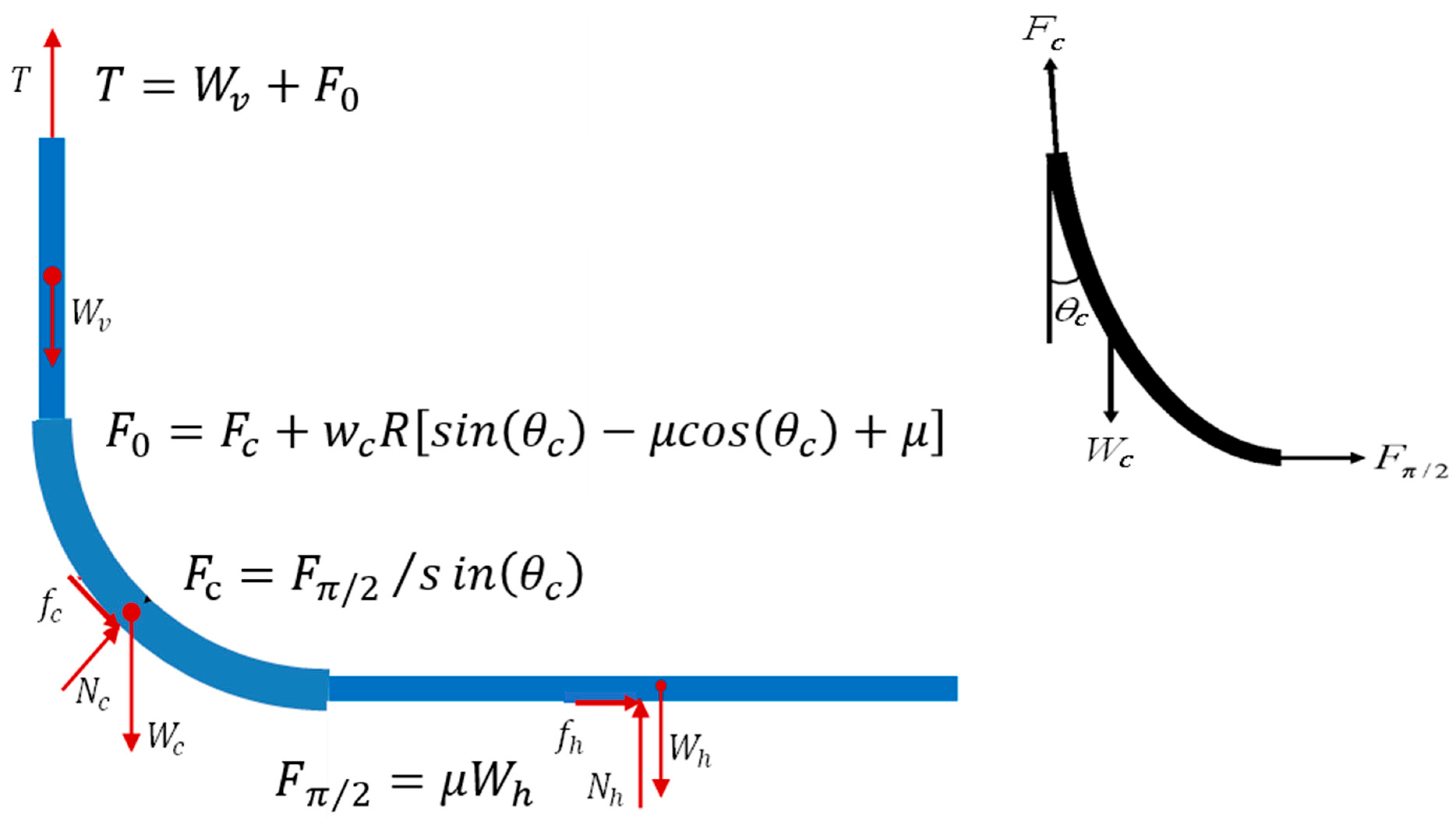
3. Prediction of Drilling Drag
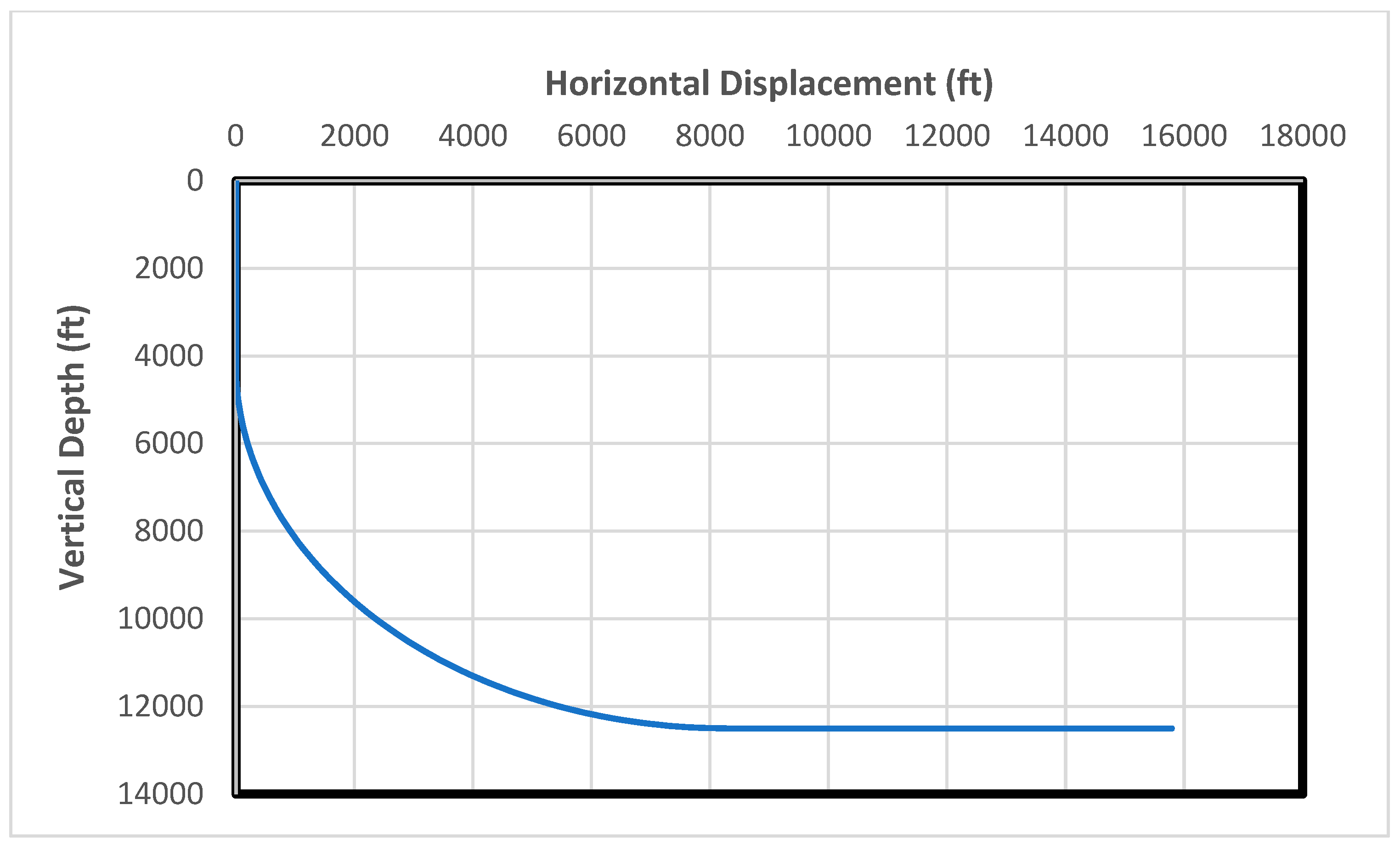
4. Field Data Study
- (1)
- Based on the past well productivity data, a horizontal wellbore length of 7500 ft is designed.
- (2)
- A catenary section is designed to have Vend = 2000 ft and Send = 4000 ft.
- (3)
- Numerical solution of Equation (1) gives a = 4297 ft.
- (4)
- Equations (2) and (3) yield a radius of curvature of 9228 ft and an inclination angle of 43° at the top end of the catenary section.
- (5)
- Equation (4) gives the vertical displacement of the arc section of 6292 ft.
- (6)
- Equation (5) results in a KOP at 4208 ft.
- (7)
- Equation (6) gives the inclination angle build rate of 0.62°/100 ft. The vertical and horizontal coordinates in the arc section are calculated based on the B-value and tabulated measured depth.
- (8)
- The vertical and horizontal coordinates in the catenary section are calculated based on the inclination angle given by Equation (7) as a function of tabulated measured depth.
- (9)
- The vertical and horizontal coordinates in the horizontal section are calculated based on the maximum inclination angle of 90°.
5. Discussion
6. Conclusions
- (1)
- The mathematical model of catenary trajectory contains closed-form equations for the radius of curvature and inclination angle in the catenary section. Using the radius of curvature at the top point of the catenary section to design the arc-section below the KOP eliminates the trial-and-error procedure required for achieving smooth transition between the two trajectory sections.
- (2)
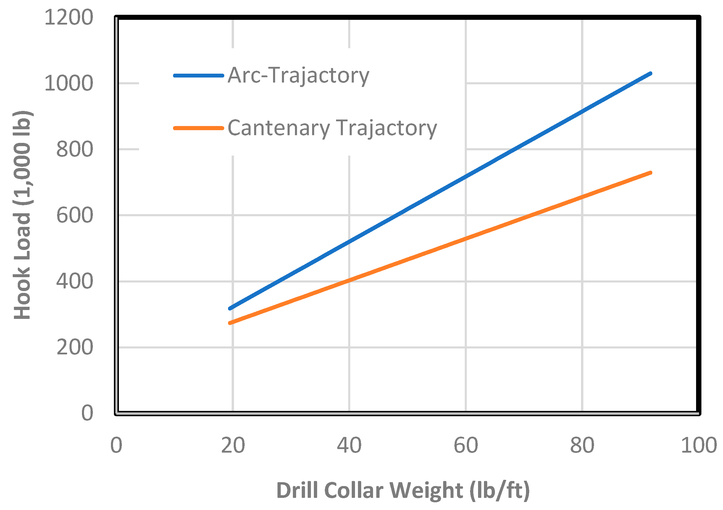
- The result of the field case study with Tuscaloosa Marine Shale (TMS) data shows that the drilling drag (hook load) can be reduced by 15% to 30% with the use of a catenary-type trajectory to replace an arc-type trajectory.
- (3)
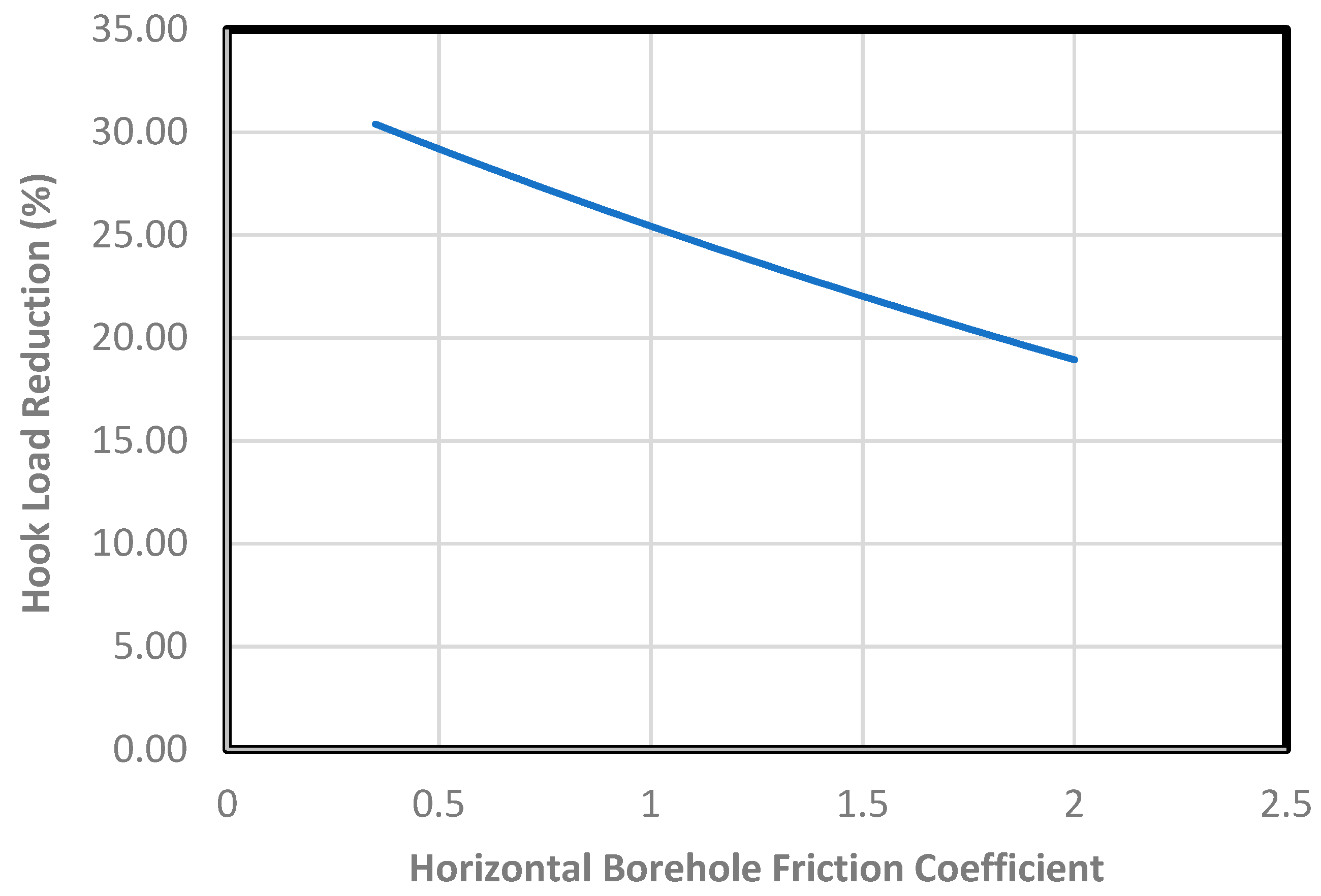
- The reduction in the hook load depends on the degree of wellbore clogging. The reduction drops linearly from 30% to 20%, with the clog indicator increasing from 0.35 to 2.0.
- (4)
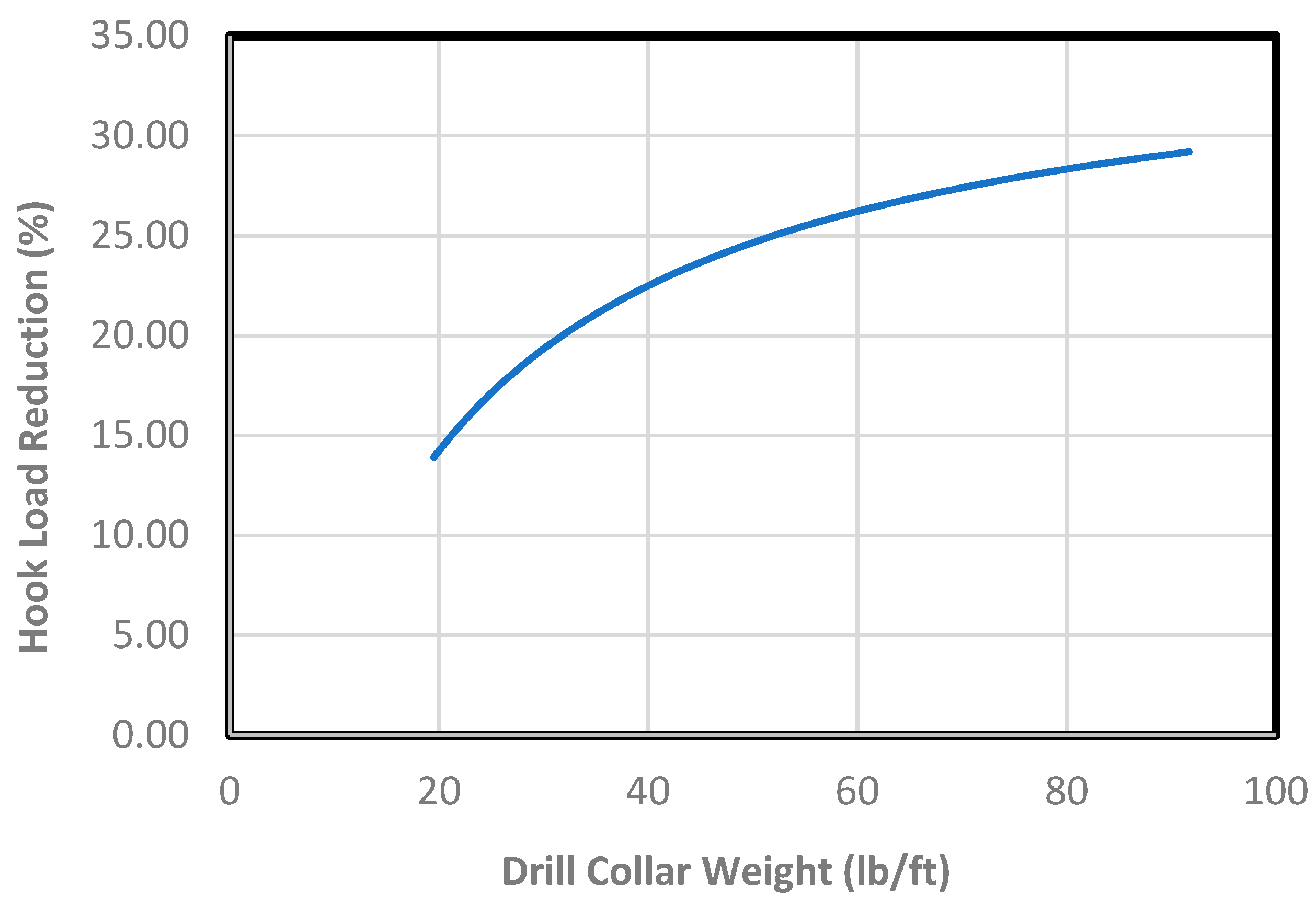
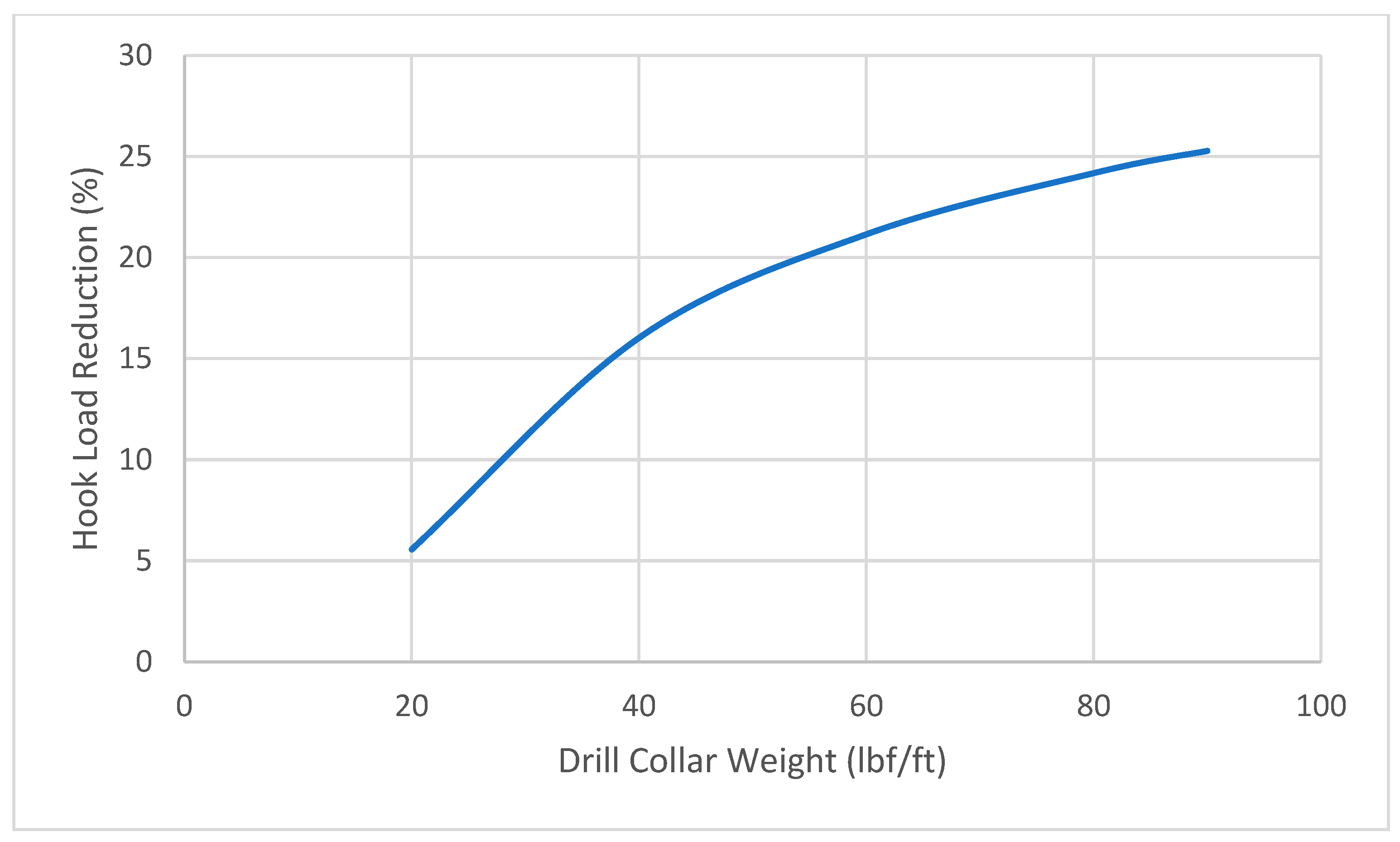
- The reduction in the hook load increases non-linearly from 15% to 30% with drill collar weight increasing from 20 lb/ft to 90 lb/ft.
Author Contributions
Funding
Data Availability Statement
Conflicts of Interest
Appendix A. Mathematical Formulation of Catenary Well Trajectory Section
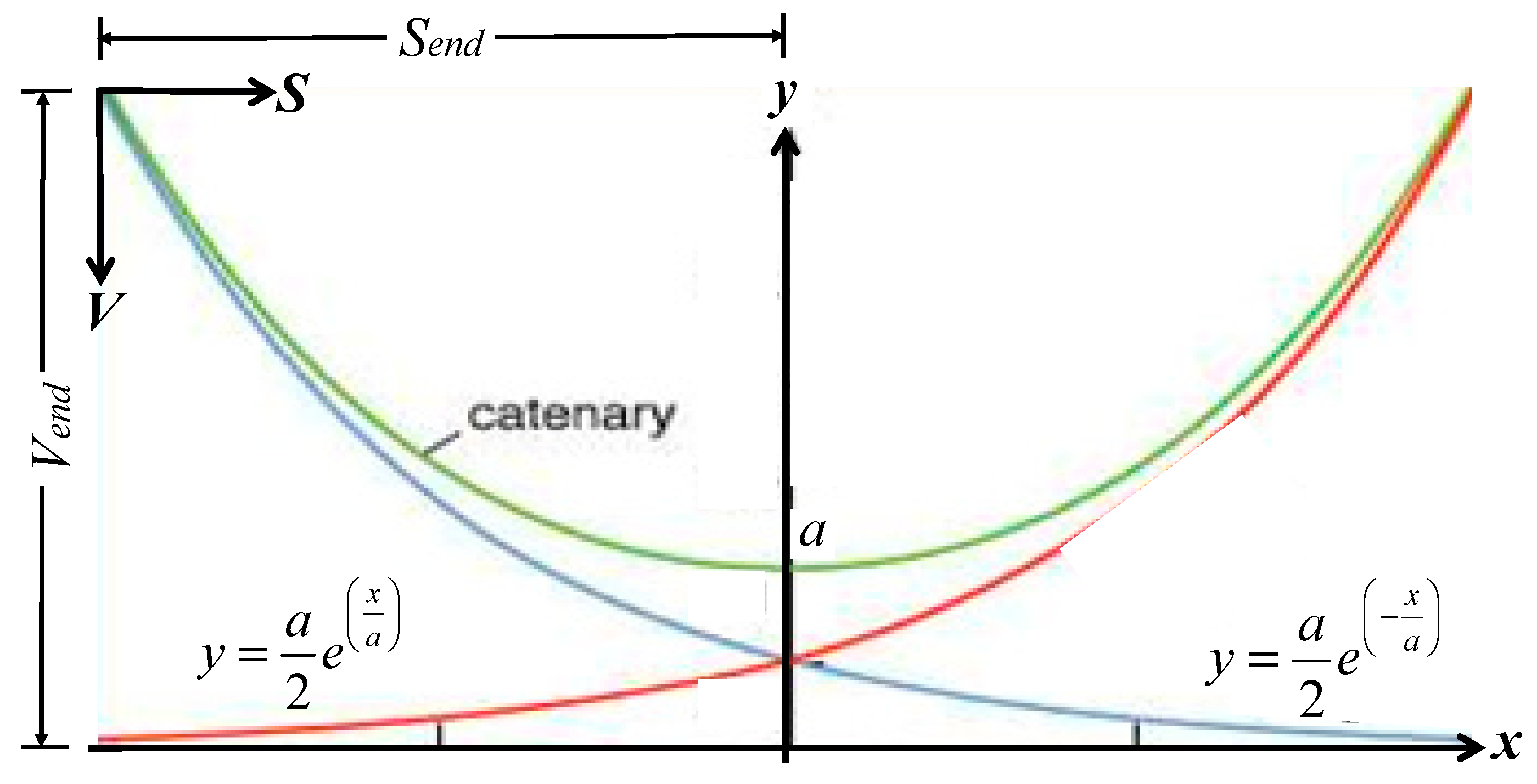
- Send is the total horizontal displacement in the catenary section,
- Vend is the total vertical displacement in the catenary section
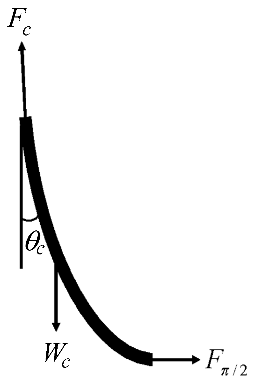
Appendix B. Derivation of Axial Force Equation for a Rope-like String in an Arc Hole

References
- Li, J.; Mang, H.; Sun, T.; Song, Z.; Gao, D. Method for designing the optimal trajectory for drilling a horizontal well, based on particle swarm optimization (PSO) and analytic hierarchy process (AHP). Chem. Technol. Fuels Oils 2019, 55, 105–115. [Google Scholar] [CrossRef]
- Huang, W.; Wu, M.; Chen, L.; She, J.; Hashimoto, H.; Kawata, S. Multi-objective drilling trajectory optimization considering parameter uncertainties. IEEE Trans. Syst. Man Cybern. Syst. 2020, 52, 1224–1233. [Google Scholar] [CrossRef]
- Wiśniowski, R.; Skrzypaszek, K.; Łopata, P.; Orłowicz, G. The Catenary Method as an Alternative to the Horizontal Directional Drilling Trajectory Design in 2D Space. Energies 2020, 13, 1112. [Google Scholar] [CrossRef]
- Sheppard, M.C.; Wick, C.; Burgess, T. Designing well paths to reduce drag and torque. SPE Drill. Eng. 1987, 2, 344–350. [Google Scholar] [CrossRef]
- Oyedere, M.; Gray, K.E. New approach to stiff-string torque and drag modeling for well planning. J. Energy Resour. Technol. 2020, 142, 103004. [Google Scholar] [CrossRef]
- Jeong, J.; Lim, C.; Park, B.C.; Bae, J.; Shin, S.C. Multi-objective optimization of drilling trajectory considering buckling risk. Appl. Sci. 2022, 12, 1829. [Google Scholar] [CrossRef]
- Qin, J.; Liu, L.; Xue, L.; Chen, X.; Weng, C. A New Multi-Objective Optimization Design Method for Directional Well Trajectory Based on Multi-Factor Constraints. Appl. Sci. 2022, 12, 10722. [Google Scholar] [CrossRef]
- McClendon, R.T.; Anders, E.O. Directional drilling using the catenary method. In Proceedings of the SPE/IADC Drilling Conference and Exhibition, New Orleans, LA, USA, 6–8 March 1985; p. SPE-13478. [Google Scholar]
- Aldaz-Saca, N.H.; Gregori, S.; Gil, J.; Tur, M.; Fuenmayor, F.J. Cantilever modelling in the railway catenary shape-finding problem. Eng. Struct. 2024, 316, 118557. [Google Scholar] [CrossRef]
- Li, Z.; Lee, T.U.; Pietroni, N.; Snooks, R.; Xie, Y.M. Design and construction of catenary-ruled surfaces. Structures 2024, 59, 105755. [Google Scholar] [CrossRef]
- Fallacara, G.; Cavaliere, I.; Melchiorre, J.; Marano, G.C.; Manuello, A. Reinterpretation of catenary vaulted spaces: Construction of a prototype and structural evaluation through Multibody Rope Approach. Structures 2024, 66, 106746. [Google Scholar] [CrossRef]
- Du, C.W.; Zhang, Y.J. The New Technology in Directional Drilling Catenary Profile. Oil Drill. Prod. Technol. 1987, 9, 17–22. [Google Scholar]
- Han, Z.Y. The Method of Practical Design of Catenary-shape Profile. Oil Drill. Prod. Technol. 1987, 9, 11–17. [Google Scholar]
- Payne, M.L.; Cocking, D.A.; Hatch, A.J. Critical Technologies for Success in Extended Reach Drilling. In Proceedings of the Paper SPE 28293 Presented at the SPE Annual Technical Conference and Exhibition, New Orleans, LA, USA, 25–28 September 1994. [Google Scholar]
- Liu, X.; Samuel, R. Catenary well profiles for ultra-extended-reach wells. In Proceedings of the SPE Annual Technical Conference and Exhibition, New Orleans, LA, USA, 3 October 2009. [Google Scholar]
- Aadnoy, B.S.; Fabiri, V.T.; Djurhuus, J. Construction of Ultra-long Wells Using a Catenary Well Profile. In Proceedings of the Paper SPE 98890 Presented at the IADC/SPE Drilling Conference, Miami, FL, USA, 21–23 February 2006. [Google Scholar]
- Song, Z.; Gao, D.; Li, R. Summary and Optimization of Extended-Reach-Well Trajectory Design Method. J. Pet. Drill. Technol. 2006, 34, 24–27. [Google Scholar]
- Wiktorski, E.; Kuznetcov, A.; Sui, D. ROP optimization and modeling in directional drilling process. In Proceedings of the SPE Norway Subsurface Conference, Bergen, Norway, 5 April 2017; p. D011S003R002. [Google Scholar]
- Aadnøy, B.S.; Andersen, K. Design of oil wells using analytical friction models. J. Pet. Sci. Eng. 2006, 32, 53–71. [Google Scholar] [CrossRef]
- Ramba, V.; Selvaraju, S.; Subbiah, S.; Palanisamy, M. A Robust Anomaly Detection Methodology Using Predicted Hookload and Neutral Point for Oil Well Drilling. J. Pet. Sci. Eng. 2020, 195, 107787. [Google Scholar] [CrossRef]
- John, C.J.; Jones, B.L.; Moncrief, J.E.; Bourgeois, R.; Harder, B.J. An unproven unconventional seven-billion-barrel oil resource-the Tuscaloosa Marine Shale. LSU Basin Res. Inst. Bull. 1997, 7, 1–22. [Google Scholar]
- Liu, N. Tuscaloosa Marine Shale Laboratory. In Final Report for U.S. DOE Project No. DE-FE0031575; University of Louisiana at Lafayette: Lafayette, LA, USA, 2022. [Google Scholar]


| Parameters | Vertical Section | Curve Section | Horizontal Section |
|---|---|---|---|
| Length (ft) | 4208 | 7500 | |
| Pipe outer diameter (in.) | 5.00 | 6.50 | 5.00 |
| Pipe inner diameter (in.) | 4.21 | 2.81 | 4.35 |
| Pipe unit weight (lb/ft) | 19.50 | 19.5~91.69 | 16.25 |
| Pipe cross-sectional area (in2) | 5.73 | 26.96 | 4.78 |
| Fluid density (ppg) | 9.00 | 9.00 | 9.00 |
| Pipe bottom depth (ft) | 4208 | 12,500 | 12,500 |
| Steel density (lb/ft3) | 490 | 490 | 490 |
| Fraction coefficient (clog indicator) | 0.35 | 0.35 | 0.50~2.0 |
| Buoyant factor | 0.89 | 0.89 | 0.89 |
Disclaimer/Publisher’s Note: The statements, opinions and data contained in all publications are solely those of the individual author(s) and contributor(s) and not of MDPI and/or the editor(s). MDPI and/or the editor(s) disclaim responsibility for any injury to people or property resulting from any ideas, methods, instructions or products referred to in the content. |
© 2025 by the authors. Licensee MDPI, Basel, Switzerland. This article is an open access article distributed under the terms and conditions of the Creative Commons Attribution (CC BY) license (https://creativecommons.org/licenses/by/4.0/).
Share and Cite
Guo, B.; Nguyen, V.; Lee, J. Mathematical Modeling of Friction Reduction in Drilling Long Horizontal Wells Using Smooth Catenary Well Trajectories. Processes 2025, 13, 1573. https://doi.org/10.3390/pr13051573
Guo B, Nguyen V, Lee J. Mathematical Modeling of Friction Reduction in Drilling Long Horizontal Wells Using Smooth Catenary Well Trajectories. Processes. 2025; 13(5):1573. https://doi.org/10.3390/pr13051573
Chicago/Turabian StyleGuo, Boyun, Vu Nguyen, and Jim Lee. 2025. "Mathematical Modeling of Friction Reduction in Drilling Long Horizontal Wells Using Smooth Catenary Well Trajectories" Processes 13, no. 5: 1573. https://doi.org/10.3390/pr13051573
APA StyleGuo, B., Nguyen, V., & Lee, J. (2025). Mathematical Modeling of Friction Reduction in Drilling Long Horizontal Wells Using Smooth Catenary Well Trajectories. Processes, 13(5), 1573. https://doi.org/10.3390/pr13051573