Abstract
The proton exchange membrane water electrolysis (PEMWE) technology is a highly promising method for hydrogen production. The flow field structure is a key factor affecting the electrolyzer’s performance and overall cost. The commonly used flow field designs are typically parallel flow fields or serpentine flow fields. However, parallel flow fields often suffer from an uneven distribution of reactants, which can negatively impact electrolyzer performance. Serpentine flow fields, on the other hand, exhibit higher pressure drops, leading to increased energy consumption. Furthermore, research on circular planar flow field designs in PEMWE has been limited. Therefore, this study proposes a novel annular flow field design based on a circular plane using Murray’s branching law, with comparative analysis against parallel and serpentine flow fields. This design aims to address the aforementioned issues. A three-dimensional numerical model coupling multiple physical fields was developed with the aim of verifying the effectiveness of the annular flow field design in terms of pressure drop, velocity distribution, temperature distribution, hydrogen distribution, and polarization curves. To confirm the model’s reliability, bipolar plates with the novel annular flow field were fabricated and assembled into a single cell for validation. The results show that the novel annular flow field exhibits optimal electrolytic performance and can significantly improve the uniformity of flow and temperature distribution in PEMWE. At a voltage of 2.6 V, the current density increased by 29.99% and 13.84% compared to the parallel and serpentine flow fields, respectively. The velocity distribution was the most uniform, and the average temperature of the Membrane Electrode Assembly (MEA) decreased by approximately 6.08 K and 6.84 K compared to the parallel and serpentine flow fields, respectively. Notably, the pressure drop of the annular flow field was significantly reduced, with reductions of 53.63% and 46.09% compared to the parallel and serpentine flow fields, respectively. This study provides an effective solution for the design of circular plane flow fields in PEMWE.
1. Introduction
As global energy demand continues to rise, excessive reliance on fossil fuels has led to severe air pollution and climate change issues [1,2]. In this context, the potential application of hydrogen as a clean energy carrier has attracted significant attention, and it is expected to help alleviate the current energy crisis [3]. The conversion of renewable energy electricity into green hydrogen through the electrolysis of water, and its promotion in diverse applications in industries such as manufacturing, transportation, and energy storage, is widely regarded as a key method for achieving carbon neutrality goals [4,5,6]. PEMWE (proton exchange membrane water electrolysis) is an efficient hydrogen production technology with a promising future, as it can be coupled with distributed renewable energy generation systems to produce hydrogen, providing grid load leveling and absorbing excess solar and wind power [7]. This technology offers several advantages, including high hydrogen purity, high current density, a fast dynamic response, and a compact structure [8].
Despite the advantages of PEMWE in multiple aspects, there is still room for improvement, particularly in terms of cost and durability. One possible strategy is to optimize the distribution of heat and water within the electrolyzer. The uniform distribution of liquid water is a key factor in achieving efficient mass transfer and heat dissipation, primarily due to its dual functional characteristics as both a reactant medium and a cooling medium in the reaction system [9]. The flow field configuration plays a key role in influencing the water, thermal, and polarization performance within PEMWE, and it is usually achieved by grooving the bipolar plates (BP), which are worth noting as they account for approximately 30~40% of the electrolyzer’s cost [10]. The uneven distribution of reactants can lead to the imbalanced utilization of precious catalysts, reducing the overall performance of the system. Furthermore, uneven temperature distribution can result in localized overheating, shortening the lifespan of the electrolyzer [11]. Considering these factors, a reasonable flow field configuration should be able to form a uniform water distribution, reduce the occurrence of local hot spots, and ensure even catalyst utilization.
A large body of literature describes research based on different flow field models, but existing results are mostly limited to rectangular geometric configurations. Nie et al. [12] conducted numerical and experimental studies on the parallel flow field in PEMWE, revealing an uneven velocity distribution in which the minimum velocity occurs in the central area of the flow field and the maximum velocity occurs at the inlet. This configuration has a low pressure drop, maintaining a relatively consistent pressure level, thus reducing flow turbulence and velocity [2]. Nevertheless, Ruiz et al. [13] found that the hydrogen distribution in parallel flow fields is uneven due to low flow rates and an uneven velocity distribution.
The design of serpentine flow fields enhances the uniformity of hydrogen production, current density, and temperature. In fact, the PEMWE with a single serpentine flow field is considered to be the most promising; however, the application of serpentine flow fields often exacerbates pressure loss [14]. Compared to parallel flow fields, the serpentine flow field exhibits more uniform temperature distribution, thereby reducing thermal stress and extending the membrane’s lifespan. Of course, serpentine flow fields with different numbers of channels also exhibit different performance characteristics. Toghyani et al. [11] conducted numerical simulations of single-, double-, triple-, and quadruple-channel serpentine flow fields, finding that the single-channel serpentine flow field has the best current density distribution and a higher hydrogen production rate, but a higher pressure drop that exacerbates the excess power consumption of the peristaltic pump bringing water into the channels. As the number of channels increases, the bends in the flow field decrease, and the pressure drop tends to reduce. Thus, from the perspective of hydrogen production rate, temperature distribution uniformity, and reasonable pressure drop, the conclusion was drawn that a double-channel serpentine flow field is optimal.
Additionally, some novel flow fields have been proposed. Rui Lin et al. [15] proposed a dot-patterned flow field, and through comparisons with parallel and serpentine flow fields, they found that the pressure distribution in the middle of the dot-patterned flow field is uniform, but it varies significantly at the inlet and outlet. Wang et al. [16] proposed a new interdigital flow field, and by comparing it to the parallel flow field and conventional interdigital flow field, they found that the new interdigital flow field helps improve liquid saturation, temperature distribution, and current distribution uniformity. Li et al. [17] proposed a cascaded flow field structure, and their results indicated that this configuration has advantages in reducing bubble accumulation. Toghyani et al. [18] proposed a spiral flow field, and their results demonstrated that the flow field has good uniformity in current density and temperature distribution. In their other related study [11], foam metal was used as the flow field material. This structure, with its advantages such as low temperature gradient, uniform current density distribution, high hydrogen production efficiency, and low pressure drop, demonstrated excellent electrochemical performance.
The existing literature shows that most of the research on novel flow field proposals has focused on square planes, while studies on flow field patterns in circular planes in PEMWE are severely lacking. In the limited research on circular flow patterns, Olesen et al. [9] conducted a numerical study on the anode flow field of PEMWE, and their results suggested that due to improper velocity distribution in the flow field, a circular planar interdigital flow field was proposed to replace parallel channels for more efficient reactant distribution. Hassan et al. [19] conducted a comprehensive analysis of five circular serpentine flow patterns using a three-dimensional, two-phase, non-isothermal PEMWE model, concluding that reducing the velocity, the path length, and the number of flow field bends effectively reduces the pressure drop. Minjeong Jo et al. [20] found that the use of circular bipolar plates, compared to square bipolar plates, can reduce the weight by 0.4%, and can also be applied in high-pressure electrolyzers. This verifies the unique advantages of the circular flow field in industrial-scale electrolyzers.
It is clear from past literature that there has been significant interest in designing flow fields for square-shaped geometries in PEMWE. However, there is a significant research gap in exploring flow field models based on circular plane designs. In light of this, this study attempts to fill this gap by investigating various circular flow modes. The design of the flow field in this paper takes into account Murray’s law [21], and a new circular flow field structure is proposed. The performance of this new flow field is compared with parallel and serpentine flow fields on a circular plane in terms of pressure distribution, velocity distribution, temperature distribution, hydrogen distribution, and polarization curves, proving its unique advantages.
2. Model Description
2.1. Physical Model
The flow field design in this study is based on Murray’s law. According to Murray’s law, when fluid flows through a branched channel structure, the energy consumption and pressure drop during the flow process are relatively low when there is a specific relationship between the diameters of the main and subsidiary channels in the branching system. Based on this theory, a new flow field was designed for a circular plane, and the newly proposed flow field can be referred to as an annular flow field. The width of the smallest ring is called , and the naming convention for each outer ring follows accordingly. There are also intersection points between each ring, where the width of the intersection is equal to the width of the previous ring, and so on.
In the derivative extension of Murray’s law, this can be expressed as follows:
In the formula, D0 represents the diameter of the initial pipe, Dk represents the diameter of the next level pipe, and k ≥ 1.
If the number of branches in the next level is two and the diameters of the branches are the same, it can be simplified as follows:
Since the cross-sectional shape of the flow channel is non-circular, let A represent the cross-sectional area of the flow channel, and P represent its perimeter; then, its equivalent diameter is calculated using the following formula:
Thus, the specific geometric parameters of each ring in the annular flow field can be obtained, as shown in Figure 1.
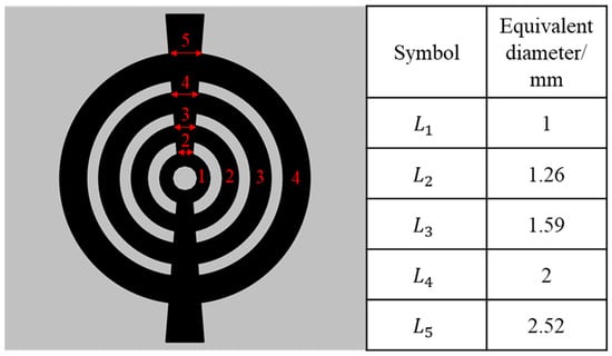
Figure 1.
Schematic diagram of the annular flow field.
The computational domain of the PEMWE model with the annular flow field is shown in Figure 2. The computational domain includes the proton exchange membrane (PEM), anode flow channel (ACH), cathode flow channel (CCH), anode catalyst layer (ACL), cathode catalyst layer (CCL), anode gas diffusion layer (AGDL), and cathode gas diffusion layer (CGDL). During operation, liquid water is introduced into the ACH and then distributed through the flow field into the porous AGDL. It then reaches the PEM loaded with catalysts, where water is decomposed into oxygen, hydrogen ions, and electrons. The hydrogen ions pass through the PEM to the cathode, where they combine with the electrons from the external circuit to produce hydrogen.

Figure 2.
Schematic diagram of the computational domain of the PEMWE model with the annular flow field.
To study the performance of the annular flow field (referred to as Model C), a parallel flow field (referred to as Model A) and a serpentine flow field (referred to as Model B) were also constructed based on a circular plane for comparison, as shown in Figure 3. The detailed geometric parameters are listed in Table 1.
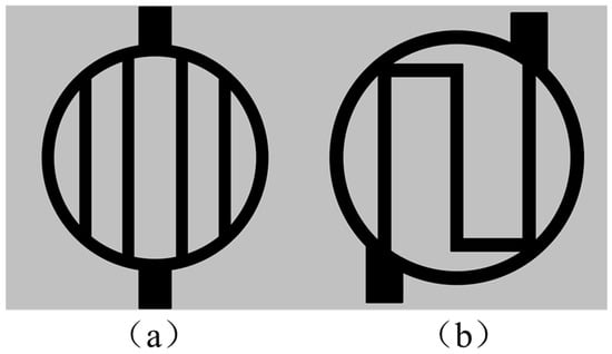
Figure 3.
Two-dimensional schematic diagrams of different flow field types, including (a) parallel flow field; (b) serpentine flow field.

Table 1.
Geometric parameters of the PEMWE.
2.2. Model Assumptions
The simulation of PEMWE involves multiple physical fields and complex computational processes, including equations for charge conservation, mass transfer, and momentum conservation. To simplify the model and improve convergence, the following assumptions are made [22,23]:
- Steady-state conditions and laminar flow are considered.
- The catalyst layer and porous media in the model are assumed to be isotropic and homogeneous.
- Only hydrogen ions are allowed to pass through the PEM, while cross-diffusion of hydrogen and oxygen is neglected.
- Contact resistance is not considered.
- The influence of gravity is ignored.
2.3. Numerical Model
2.3.1. Electrochemical Model
The electrolysis voltage E during the hydrogen production process of a proton exchange membrane water electrolyzer consists of the open-circuit voltage , activation overpotential , and ohmic overpotential [24,25].
The open-circuit voltage can be calculated using the Nernst equation:
where R is the gas constant, n is the number of electrons, F is the Faraday constant, and T is the operating temperature. (i representing O2, H2, H2O) is the equilibrium pressure of each component. can be calculated using the following formula:
The activation overpotentials for the anode and cathode can be calculated using the Butler–Volmer equation [26,27]:
where is the active surface area, and are the charge transfer coefficients, and and are the exchange current densities for the anode and cathode. The exchange current density can be calculated using the following equation [28]:
where represents the activation energy, and is the reference exchange current density.
When electrons are transferred between the cells, part of the energy is lost, which is referred to as ohmic losses, primarily generated by the resistance between various parts. The electron transfer equation can be described as follows [29]:
where is the electron potential, represents the rate of electron loss in the electrochemical reaction, and is the effective conductivity of the solid region. The diffusion layer and catalyst layer are defined as homogeneous for each phase, so = . Therefore, the ohmic overpotential can be calculated based on Ohm’s law using the following formula [30]:
2.3.2. Heat Transfer Model
During the operation of the electrolyzer, the electrochemical reactions are accompanied by both heat generation and consumption. Water electrolysis is a typical endothermic reaction, but for the electrolyzer, heat is generated due to various overpotentials. The thermal balance of the electrolyzer is described by the energy equation, which can be expressed as follows [31]:
In the equation, , , and represent the thermal conductivity, density, and heat capacity of the solid region, respectively. Similarly, , , and represent the thermal conductivity, density, and heat capacity of the fluid mixture. is the source term, which mainly includes the irreversible heat generated by the electrochemical reaction , entropy heat source , and ohmic heat generated by multiple interfaces .
2.3.3. Mass Transfer Model
The mass conservation equation and momentum conservation equation are used to describe the mass transfer of the mixture within the electrolyzer [25,32]:
where represents the porosity of the porous medium, and its value is 1. and represent the viscosity and average density of the mixture, respectively. is the source term, and is the volume-averaged velocity of the mixture [33]:
where , , and represent the volume, density, and velocity of substance (k), respectively.
Gas–liquid flow in porous media is complex, and the Maxwell–Stefan equation is commonly used to describe the convection and diffusion of each component [28]:
where represents the molar concentration of component (k) and is the effective diffusion coefficient, which can be corrected by Bruggeman’s equation:
is a function of temperature and pressure:
where represents the diffusion coefficient of the binary component at reference conditions.
Table 2 summarizes the values of the physical parameters used in the model.
Table 2.
Physical parameters in the model.
2.3.4. Boundary Conditions
The boundary condition at the water inlet on the anode side of the flow channel is set as a mass flow rate of 2 × 10⁻⁵ kg/s. A no-pressure condition is applied at the outlets of both the anode and cathode flow field channels. All other surfaces, except for the inlet and outlet, are treated as no-slip walls. For heat transfer, the inlet water temperature is maintained at a constant value of 353.15 K, which is the operating temperature, while the remaining external boundaries are thermally insulated.
2.4. Numerical Process and Model Validation
2.4.1. Numerical Implementation
In this study, the multi-physics calculations were conducted using COMSOL Multiphysics 6.1 simulation software. A total of three modules were employed to model the charge transfer, heat transfer, and mass transfer phenomena. These modules included the Water Electrolyzer, Free and Porous Media Flow, and Heat Transfer in Solids and Fluids modules. To ensure optimal computational efficiency and resource utilization, the mesh was generated primarily using hexahedral and free tetrahedral elements, totaling 98,913 elements. The PARDISO direct solver was used to perform parameter sweeps and iterative calculations, continuing until the residual error was below 10−4.
2.4.2. Model Validation
To ensure the accuracy of the numerical model, the simulation results were compared with the experimental data. For this purpose, bipolar plates with three different flow field designs were fabricated, as shown in Figure 4 (manufactured by Mainz Hydrogen, Mainz, Germany), and assembled into a single cell for experimental validation. The AGDL and CGDL were made from 0.6 mm and 0.5 mm titanium felt (sourced from Suzhou Shengernuo Technology Co., Ltd., Suzhou, China), consistent with the simulation setup. The MEA was a commercial product (Chunhua Hydrogen Technology Co., Ltd., Zhuzhou, China), with an effective area cut to πcm2. An experimental system, as depicted in Figure 5, was set up, comprising an electrochemical workstation (AUTOLAB PGSTAT302N, Metrohm, Herisau, Switzerland), a PEM water electrolyzer, an anode water tank, and a peristaltic pump. Before the electrochemical tests, 80 °C deionized water was pumped into the electrolyzer for half an hour via the peristaltic pump, which helped to increase the electrolyzer’s temperature and ensure that the membrane remained water-saturated.

Figure 4.
Photographs of bipolar plates with different flow field shapes: (a) parallel flow field; (b) serpentine flow field; (c) annular flow field.
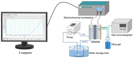
Figure 5.
Schematic diagram of the experimental system for PEMWE.
Figure 6 shows the polarization curve comparison between the simulation data based on Model C and the experimental data. It is found that the error between the simulation model’s calculated data and the experimental measured data is within 5%, indicating that the established model was reasonably accurate. At the same current density, the simulated voltage was slightly lower, which was mainly attributed to the neglect of contact resistance between the different interfaces.
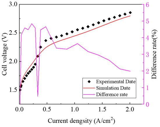
Figure 6.
Comparison of polarization curves between experimental data and simulation data.
3. Results and Discussion
The feasibility of the novel annular flow field in PEMWE was verified by comparing the performance of three different flow fields. The same design parameters and operating conditions were used for all three flow fields.
3.1. Pressure Distribution
The pressure drop in the flow field reflects the additional power consumed by the water pump in the electrolytic system to deliver water into the flow field. In Figure 7a–c, the pressure distribution for the different flow field structures can be observed. In all flow fields, the pressure gradually decreases from the inlet to the outlet, while Model C, due to its unique design, exhibits higher pressure in the inner ring and lower pressure in the outer ring. Figure 7d shows the pressure drop variations in the different flow field structures under varying current densities. As the current density increases, the pressure drop in each flow field slowly rises. Thanks to the application of Murray’s branching law in Model C, the energy loss of the fluid flowing through this type of channel is minimized, resulting in a significant reduction in pressure drop. The pressure drop magnitude is in the order of Model A > Model B > Model C.

Figure 7.
Comparison of the pressure distribution in three flow fields: (a) Model A; (b) Model B; (c) Model C. (d) Diagram showing the pressure drop in the three flow fields as a function of current density variation.
At a current density of 2 A/cm2, the pressure drops in the parallel flow field, serpentine flow field, and annular flow field are 565 Pa, 486 Pa, and 262 Pa, respectively. Compared to the other two types of flow fields, the pressure drop in the annular flow field is significantly reduced. Higher pressure drops will inevitably increase the energy consumption of the water supply in the electrolytic system. In traditional flow field structures, large areas of ribs often result in insufficient water supply to the region beneath the ribs due to the lack of direct contact between the reactants in the channel and the GDL under the ribs. This condition is detrimental to the reaction and can lead to gas accumulation, further obstructing the water supply. In contrast, the novel annular flow field significantly reduces the pressure drop level, and its special structure minimizes the rib area, which is beneficial for the reaction process.
3.2. Velocity Distribution
Flow velocity plays a crucial role in the electrolytic system for both the feed of reactants and the rapid discharge of generated oxygen. Therefore, the distribution of water flow velocity significantly influences the electrolysis process in PEMWE. Uneven flow distribution may lead to imbalanced utilization of the catalyst. Figure 8a–c show the velocity distribution within the channels of different flow field structures. The maximum velocities in the parallel, serpentine, and annular flow fields are 23.9 m/s, 23.5 m/s, and 19.9 m/s, respectively. The parallel flow field exhibits the highest velocity because its unobstructed structure facilitates rapid fluid passage, but this also hinders the diffusion of reactants towards the catalyst layer. The serpentine flow field has slightly lower velocity due to increased flow resistance at the turns. The annular flow field, with its unique structure, has the lowest velocity, which allows reactants to remain in the flow field for a longer time, enabling more complete reactions.
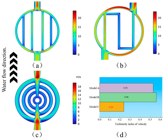
Figure 8.
Distribution of water flow velocity in three flow fields: (a) Model A; (b) Model B; (c) Model C. (d) Comparison of the uniformity index for the three flow fields.
At the same time, Figure 8d introduces a uniformity index to analyze the velocity distribution uniformity of the three flow field structures. The uniformity index is represented by the following equation [28]:
where and represent the local velocity and the average velocity, respectively. As the uniformity index decreases, the velocity distribution becomes more uniform. In other words, when the uniformity index is zero, the velocity distribution is completely uniform. The annular flow field demonstrates the most uniform velocity distribution, allowing for a more evenly distributed flow field over the catalyst surface, which is conducive to the reaction process.
3.3. Temperature Distribution
The electrochemical reaction during water electrolysis is an exothermic process, accompanied by heat generation, leading to localized temperature increases. Although the rise in temperature benefits the electrochemical reaction, excessive localized heat can result in thermal stress, potentially causing PEM failure and catalyst deactivation, thereby severely impacting the lifespan and stability of the electrolytic system. Therefore, effective thermal management of the electrolyzer is crucial.
Figure 9 shows the temperature distribution in the YZ direction of the PEMWE with different flow field structures. A YZ direction section is taken at equal intervals, clearly displaying the temperature distribution of various components of the electrolyzer from top to bottom. It can be seen that at the inlet, the color is purple, indicating a relatively low temperature, while at the outlet, the color is red, indicating a relatively high temperature. It can be seen that the temperature gradually increases from the inlet to the outlet, mainly due to the heat generated during the operation of the electrolyzer and the reduced liquid water content near the outlet. The highest temperature occurs at the center of the electrochemical reaction, i.e., between the CL and the PEM.
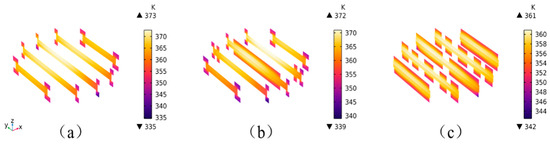
Figure 9.
Temperature variation of PEMWE under different flow field structures (YZ section from inlet to outlet): (a) Model A; (b) Model B; (c) Model C.
Figure 10 illustrates the temperature distribution at the CL–PEM interface for different flow field structures. It can be observed that the uniform velocity distribution in the flow field in Model C leads to a more uniform temperature distribution, which can reduce thermal stress, extend the membrane’s lifespan, and decrease system energy loss. Additionally, the application of the annular flow field reduces the temperature at the CL–PEM interface; the average temperature of the MEA is approximately 6.08 K and 6.84 K lower compared to the parallel and serpentine flow fields, respectively. This reduction is due to the increased retention time of liquid water in the annular flow field, allowing more water to reach the reaction interface. Here, water serves both as a reactant and a coolant, effectively lowering the temperature at the CL–MEA interface. As shown in Figure 11, the reduction in oxygen mass fraction within the GDL decreases the likelihood of oxygen clogging the porous medium, further facilitating the transport of water to the reaction interface, resulting in an additional temperature decrease. Moreover, the thermal conductivity of liquid water is significantly higher than that of gas, so a reduction in oxygen content in the flow field corresponds to an increase in liquid water content; this increased water content helps to dissipate heat from the electrolyzer. Utilizing the annular flow field for gas–liquid mass transfer significantly enhances the thermal management of the electrolyzer, preventing localized overheating.

Figure 10.
Temperature distribution at the CL–PEM interface for different flow field structures: (a) Model A; (b) Model B; (c) Model C.

Figure 11.
Average temperature of the MEA and oxygen mass fraction in the GDL.
3.4. Hydrogen Distribution
Figure 12a–c illustrate the distribution of the hydrogen mass fraction on the cathode side for the various flow field structures. In all configurations, the hydrogen mass fraction increases gradually from the inlet to the outlet. Figure 12d further demonstrates the changes in hydrogen mass fraction across the different flow fields as the current density rises from 1.6 to 2 A/cm2. It is evident that as the current density increases, the hydrogen production rate also increases, highlighting a strong correlation between hydrogen production and current density. At the same current density, the hydrogen production rate follows this order: annular flow field > serpentine flow field > parallel flow field. This can be attributed to the more uniform velocity distribution in the annular flow field, which ensures more balanced catalyst utilization and, consequently, higher hydrogen production. In contrast, the higher velocity in the parallel flow field impedes the movement of liquid water to the CL, resulting in a lower hydrogen production rate.

Figure 12.
Distribution of hydrogen in different flow field structures on the cathode side: (a) Model A; (b) Model B; (c) Model C. (d) Schematic diagram of the variation in hydrogen mass fraction with current density for the three flow fields.
3.5. Comparison of Polarization Curves
Through the experimental assembly of the bipolar plate testing fixture, this study obtained the polarization curve shown in Figure 13a. It can be observed that in all cases, the current density increases with the rise in voltage. The annular flow field exhibits the best polarization performance. Figure 13b presents a comparison of current densities under the different flow field structures at 2.6 V. At this voltage, the current densities for flow field types A, B, and C are 0.9554 A/cm2, 1.091 A/cm2, and 1.242 A/cm2, respectively. The current density of type C is 29.99% and 13.84% higher than that of types A and B, respectively. This suggests that the use of the annular flow field can significantly enhance the performance of the electrolyzer. The improvement is primarily attributed to the lower pressure drop of the annular flow field, which facilitates the entry of liquid water. Additionally, it ensures a more uniform distribution of both liquid water and temperature, thereby promoting the efficient removal of gaseous products. This, in turn, prevents the buildup of mass transfer overpotentials and allows liquid water to rapidly reach the reaction interface.

Figure 13.
(a) Comparison of polarization curves; (b) Comparison of current density in electrolyzer cells assembled with different flow-field bipolar plates under 2.6 V voltage.
3.6. Potential Problems in the Design of Annular Flow Fields
Despite the relatively excellent performance demonstrated by the design of annular flow fields in various aspects, there are still some issues. On one hand, this study ensures that the reaction area (MEA area) of each flow field is the same as a basis for comparison, to ensure consistency in the catalyst content, which has the most significant impact during the electrolysis process. However, this may not be comprehensive. For example, one possible influencing factor is that, due to the unique design of the annular flow field, the total area of its flow channels is larger than that of the other two types of flow fields, which could have a certain impact on the results. On the other hand, the processing of annular flow fields is relatively complex, which may add to the cost burden of the PEMWE.
4. Conclusions
By establishing a three-dimensional numerical model, we investigated the feasibility of applying the novel annular flow field in PEMWE and fabricated a bipolar plate with the annular flow field to assemble an electrolyzer, validating the effectiveness of the simulation. The performance impact of the new annular flow field was compared with parallel and serpentine flow fields based on circular plane designs in PEMWE. The results show the following:
- The novel annular flow field, through the application of Murray’s branching law, exhibits excellent pressure drop characteristics. At a current density of 2 A/cm2, the pressure drop is reduced by 53.63% and 46.09% compared to the parallel and serpentine flow fields, respectively, which is significantly lower than the other two flow field types.
- In addition, the annular flow field demonstrates superior flow characteristics, forming a uniform water distribution that effectively avoids uneven catalyst utilization.
- The uniform water distribution in the annular flow field also improves the thermal management of the electrolyzer. After applying the annular flow field, the temperature at the CL–PEM interface is significantly reduced; the average temperature of the MEA is lowered by approximately 6.08 K and 6.84 K compared to the parallel and serpentine flow fields, respectively.
- The excellent flow and heat transfer characteristics of the annular flow field provide favorable conditions for electrochemical reactions, leading to better electrolysis performance and higher hydrogen production rates. At 2.6 V, the current density of the annular flow field is increased by 29.99% and 13.84% compared to the parallel and serpentine flow fields, respectively.
Author Contributions
Conceptualization, R.M., Y.H. and Z.W.; Methodology, R.M. and Y.Z.; Software, R.M.; Validation, R.M.; Writing—original draft, R.M.; Writing—review & editing, R.M., Y.H. and Z.W.; Visualization, R.M.; Supervision, X.C. and Z.W.; Project administration, X.C., Y.Z., Y.H. and Z.W.; Funding acquisition, X.C., Y.H. and Z.W. All authors have read and agreed to the published version of the manuscript.
Funding
This research was funded by the National Natural Science Foundation of China (52125605), and the Zhejiang Provincial Natural Science Foundation of China (LR23E060001).
Data Availability Statement
The original contributions presented in this study are included in the article. Further inquiries can be directed to the corresponding author.
Conflicts of Interest
Authors Rui Mu, Xiaoyu Cao, and Yi Zhang were employed by the company CNPC Baoji Oilfield Machinery Co., Ltd. The remaining authors declare that the research was conducted in the absence of any commercial or financial relationships that could be construed as a potential conflict of interest. The company had no role in the design of the study; in the collection, analyses, or interpretation of data; in the writing of the manuscript, or in the decision to publish the results.
References
- Hannan, M.A.; Lipu, M.S.H.; Ker, P.J.; Begum, R.A.; Agelidis, V.G.; Blaabjerg, F. Power electronics contribution to renewable energy conversion addressing emission reduction: Applications, issues, and recommendations. Appl. Energy 2019, 251, 113404. [Google Scholar] [CrossRef]
- Esquivel-Patiño, G.G.; Serna-González, M.; Nápoles-Rivera, F. Thermal integration of natural gas combined cycle power plants with CO2 capture systems and organic Rankine cycles. Energy Convers. Manag. 2017, 151, 334–342. [Google Scholar] [CrossRef]
- Akyuz, E.S.; Telli, E.; Farsak, M. Hydrogen generation electrolyzers: Paving the way for sustainable energy. Int. J. Hydrogen Energy 2024, 81, 1338–1362. [Google Scholar] [CrossRef]
- Ni, A.; Upadhyay, M.; Kumar, S.S.; Uwitonze, H.; Lim, H. Anode analysis and modelling hydrodynamic behaviour of the multiphase flow field in circular PEM water electrolyzer. Int. J. Hydrogen Energy 2023, 48, 16176–16183. [Google Scholar] [CrossRef]
- Haszeldine, R.S.; Flude, S.; Johnson, G.; Scott, V. Negative emissions technologies and carbon capture and storage to achieve the Paris Agreement commitments. Philos. Trans. R. Soc. A 2018, 376, 23. [Google Scholar] [CrossRef]
- Midilli, A.; Dincer, I. Hydrogen as a renewable and sustainable solution in reducing global fossil fuel consumption. Int. J. Hydrogen Energy 2008, 33, 4209–4222. [Google Scholar] [CrossRef]
- Grigoriev, S.A.; Kalinnikov, A.A. Mathematical modeling and experimental study of the performance of PEM water electrolysis cell with different loadings of platinum metals in electrocatalytic layers. Int. J. Hydrogen Energy 2017, 42, 1590–1597. [Google Scholar] [CrossRef]
- Chen, Y.; Dai, C.; Wu, Q.; Li, H.; Xi, S.; Seow, J.Z.Y.; Luo, S.; Meng, F.; Bo, Y.; Xia, Y.; et al. Support-free iridium hydroxide for high-efficiency proton-exchange membrane water electrolysis. Nat. Commun. 2025, 16, 2730. [Google Scholar] [CrossRef]
- Olesen, A.C.; Romer, C.; Kaer, S.K. A numerical study of the gas-liquid, two-phase flow maldistribution in the anode of a high pressure PEM water electrolysis cell. Int. J. Hydrogen Energy 2016, 41, 52–68. [Google Scholar] [CrossRef]
- Li, X.; Yao, Y.; Tian, Y.; Jia, J.; Ma, W.; Yan, X.; Liang, J. Recent advances in key components of proton exchange membrane water electrolysers. Mater. Chem. Front. 2024, 8, 2493–2510. [Google Scholar] [CrossRef]
- Toghyani, S.; Afshari, E.; Baniasadi, E.; Atyabi, S.A. Thermal and electrochemical analysis of different flow field patterns in a PEM electrolyzer. Electrochim. Acta 2018, 267, 234–245. [Google Scholar] [CrossRef]
- Nie, J.; Chen, Y.; Boehm, R.F. Numerical modeling of two-phase flow in a bipolar plate of a pem electrolyzer cell. In IMECE 2008: Heat Transfer, Fluid Flows, and Thermal Systems, PTS A–C, Proceedings of the ASME 2008 International Mechanical Engineering Congress and Exposition, Boston, MA, USA, 31 October–6 November 2008; ASME: New York, NY, USA, 2009; Volume 10, pp. 783–788. [Google Scholar]
- de Haro Ruiz, D.; Sasmito, A.P.; Shamim, T. Numerical Investigation of the High Temperature PEM Electrolyzer: Effect of Flow Channel Configurations. ECS Trans. 2013, 58, 99–112. [Google Scholar] [CrossRef]
- An, Z.; Yao, M.; Du, X.; Li, Q.; Jian, B.; Zhang, D. Influence of external operating parameters on the hydrothermal transport and performance in proton exchange membrane water electrolyzer. Ionics 2025, 30, 6253–6266. [Google Scholar] [CrossRef]
- Lin, R.; Lu, Y.; Xu, J.; Huo, J.; Cai, X. Investigation on performance of proton exchange membrane electrolyzer with different flow field structures. Appl. Energy 2022, 326, 11. [Google Scholar] [CrossRef]
- Wang, X.Y.; Wang, Z.M.; Feng, Y.C.; Xu, C.; Chen, Z.C.; Liao, Z.R.; Ju, X. Three-dimensional multiphase modeling of a proton exchange membrane electrolysis cell with a new interdigitated-jet hole flow field. Sci. China Technol. Sci. 2022, 65, 1179–1192. [Google Scholar] [CrossRef]
- Li, H.; Nakajima, H.; Inada, A.; Ito, K. Effect of flow-field pattern and flow configuration on the performance of a polymer-electrolyte-membrane water electrolyzer at high temperature. Int. J. Hydrogen Energy 2018, 43, 8600–8610. [Google Scholar] [CrossRef]
- Toghyani, S.; Afshari, E.; Baniasadi, E. Three-dimensional computational fluid dynamics modeling of proton exchange membrane electrolyzer with new flow field pattern. J. Therm. Anal. Calorim. 2019, 135, 1911–1919. [Google Scholar] [CrossRef]
- Hassan, A.H.; Liao, Z.; Wang, K.; Xiao, F.; Xu, C.; Abdelsamie, M.M. Characteristics of different flow patterns for proton exchange membrane water electrolysis with circular geometry. Int. J. Hydrogen Energy 2024, 49, 1060–1078. [Google Scholar] [CrossRef]
- Jo, M.; Cho, H.S.; Na, Y. Comparative Analysis of Circular and Square End Plates for a Highly Pressurized Proton Exchange Membrane Water Electrolysis Stack. Appl. Sci. 2020, 10, 6315. [Google Scholar] [CrossRef]
- Murray, C.D. The physiological principle of minimum work applied to the angle of branching of arteries. J. Gen. Physiol. 1926, 9, 835–841. [Google Scholar] [CrossRef]
- Chen, Z.; Yin, L.; Wang, Z.; Wang, K.; Ye, F.; Xu, C. Numerical simulation of parameter change in a proton exchange membrane electrolysis cell based on a dynamic model. Int. J. Energy Res. 2022, 46, 24074–24090. [Google Scholar] [CrossRef]
- Chen, Z.; Wang, X.; Liu, C.; Gu, L.; Yin, L.; Xu, C.; Liao, Z.; Wang, Z. Numerical investigation of PEM electrolysis cell with the new interdigitated-jet hole flow field. Int. J. Hydrogen Energy 2022, 47, 33177–33194. [Google Scholar] [CrossRef]
- Han, B.; Mo, J.; Kang, Z.; Yang, G.; Barnhill, W.; Zhang, F. Modeling of two-phase transport in proton exchange membrane electrolyzer cells for hydrogen energy. Int. J. Hydrogen Energy 2017, 42, 4478–4489. [Google Scholar] [CrossRef]
- Zhang, Z.; Xing, X. Simulation and experiment of heat and mass transfer in a proton exchange membrane electrolysis cell. Int. J. Hydrogen Energy 2020, 45, 20184–20193. [Google Scholar] [CrossRef]
- Abdin, Z.; Webb, C.J.; Gray, E.M. Modelling and simulation of a proton exchange membrane (PEM) electrolyser cell. Int. J. Hydrogen Energy 2015, 40, 13243–13257. [Google Scholar] [CrossRef]
- Wang, Z.M.; Xu, C.; Wang, X.Y.; Liao, Z.R.; Du, X.Z. Numerical investigation of water and temperature distributions in a proton exchange membrane electrolysis cell. Sci. China Technol. Sci. 2021, 64, 1555–1566. [Google Scholar] [CrossRef]
- Garcia-Valverde, R.; Espinosa, N.; Urbina, A. Simple PEM water electrolyser model and experimental validation. Int. J. Hydrogen Energy 2012, 37, 1927–1938. [Google Scholar] [CrossRef]
- Freire, L.S.; Antolini, E.; Linardi, M.; Santiago, E.I.; Passos, R.R. Influence of operational parameters on the performance of PEMFCs with serpentine flow field channels having different (rectangular and trapezoidal) cross-section shape. Int. J. Hydrogen Energy 2014, 39, 12052–12060. [Google Scholar] [CrossRef]
- Aubras, F.; Deseure, J.; Kadjo, J.J.A.; Dedigama, I.; Majasan, J.; Grondin-Perez, B.; Chabriat, J.-P.; Brett, D. Two-dimensional model of low-pressure PEM electrolyser: Two-phase flow regime, electrochemical modelling and experimental validation. Int. J. Hydrogen Energy 2017, 42, 26203–26216. [Google Scholar] [CrossRef]
- Chen, Y.; Mojica, F.; Li, G.; Chuang, P.A. Experimental study and analytical modeling of an alkaline water electrolysis cell. Int. J. Energy Res. 2017, 41, 2365–2373. [Google Scholar] [CrossRef]
- Toghyani, S.; Afshari, E.; Baniasadi, E. Metal foams as flow distributors in comparison with serpentine and parallel flow fields in proton exchange membrane electrolyzer cells. Electrochim. Acta 2018, 290, 506–519. [Google Scholar] [CrossRef]
- Nie, J.; Chen, Y. Numerical modeling of three-dimensional two-phase gas-liquid flow in the flow field plate of a PEM electrolysis cell. Int. J. Hydrogen Energy 2010, 35, 3183–3197. [Google Scholar] [CrossRef]
Disclaimer/Publisher’s Note: The statements, opinions and data contained in all publications are solely those of the individual author(s) and contributor(s) and not of MDPI and/or the editor(s). MDPI and/or the editor(s) disclaim responsibility for any injury to people or property resulting from any ideas, methods, instructions or products referred to in the content. |
© 2025 by the authors. Licensee MDPI, Basel, Switzerland. This article is an open access article distributed under the terms and conditions of the Creative Commons Attribution (CC BY) license (https://creativecommons.org/licenses/by/4.0/).