Research on the Calibration of Discrete Elemental Parameters of Yam Bean Based on GA-BP Improved Neural Network Algorithm

Abstract

The yam bean lacks accurate simulation model parameters for mechanized sowing and harvesting. The absence of parameters for the simulation model can lead to low-level mechanized design of the yam bean, which greatly affects its utilization and causes a waste of resources. This paper combines physical and simulation tests to carry out discrete elemental parameter calibration of the yam bean. The data were predictively analyzed by machine learning algorithms. A determination of basic and contact parameters of the yam bean was conducted based on physical tests. A discrete elemental model of the yam bean was developed, and angle of repose discrete elemental simulation tests were performed. The selection of simulation parameters and the identification of the optimal value range for simulation parameters were carried out by the Plackett–Burman test and the steepest climb test. Central Composite Design tests were conducted, and the results were used as a dataset for machine learning regression modeling. Then, the performances of three machine learning regression models were compared—back propagation (BP), genetic algorithm back propagation (GA-BP), and particle swarm optimization back propagation (PSO-BP). The coefficient of determination (R²), mean absolute error (MSE), and mean square error (MAE) of BP were 0.9004, 0.5204, and 0.3554, respectively. The R², MSE, and MAE of GA-BP were 0.9611, 0.2112, and 0.2809, respectively. The R², MSE, and MAE of PSO-BP were 0.9485, 0.2166, and 0.2883, respectively. It was determined that the GA-BP prediction model performed better overall. To ultimately determine the ideal set of simulation parameters, the GA-BP prediction model was examined and assessed. The GA-BP prediction model’s accuracy was validated by testing, revealing an inaccuracy of 1.22% between the rest angles measured in the simulation and the physical test. The results obtained from this research can act as a theoretical premise for further exploring the sowing and harvesting mechanisms of the yam bean.

1. Introduction

Yam beans, also known as yam seeds, zero yu seeds, and plant sprouts, are an important and nutritious food. Yam beans have the same medicinal value as yams and can also be used as yam seeds. Yam beans are widely distributed in North China, Northwest China, and the Yangtze River Basin area, with high economic value and broad market prospects. The yam bean is borne in the axils of the above-ground part of the yam and falls to the ground when ripe. The mechanized planting and harvesting equipment of yam beans has rarely been studied, limiting its industrialization and resulting in a waste of food value. The swift advancement of discrete element technology in the past several years has allowed this technique to be used to analyze the interaction of yam beans during collisions with implements during planting or harvesting. The employment of discrete element technology is crucial for promoting the mechanized cultivation of yam beans and the development of harvesting implements.

In recent years, simulation and modeling techniques based on the discrete element method and EDEM software (Version: 2024.1) have been widely used in agricultural machinery research [1,2,3,4]. Calibration of discrete meta-parameters for materials such as soil, fertilizer, straw, potatoes, and seeds has been accomplished by scholars [5,6,7,8,9]. Wan et al. [10] analyzed the effects of vibration parameters and soil layer parameters on the peak soil pressure by constructing a discrete element model of low-frequency soil vibration. Duan et al. [11] constructed a discrete meta-simulation model of granular fertilizers that can produce breakage using the Hertz–Mindlin with Bonding contact model and explored the relationship between fertilizer breakage rates and key factors. Zhu et al. [12], with the aim of resolving the problem of straw clogging during no-tillage planter operation, investigated the interaction between straw–soil mixtures and anti-clogging devices through theoretical and discrete element simulation experiments. Yan et al. [13] developed a variety of discrete elemental models of horse potato soil aggregates in order to investigate the interactions between potato-crushing devices and potato soil aggregates. A multitude of studies have been undertaken with respect to the calibration of discrete element parameters for seeds of various crops, with numerous scholars conducting discrete element simulation analyses focusing on seeds, seed-planting machine interactions, and soil interactions. Fan et al. [14] developed several different multisphere models for wheat seeds based on their geometrical characteristics. Jia et al. [15] developed a discrete elemental model of different shapes of corn seeds with a new convergent groove structure seed guide in order to investigate the effect of variability in corn seed shape and seed guide tube structure on sowing uniformity. Zhu et al. [16] developed a discrete element simulation model for straw–soil equipment. The yam bean, as one of the seeds of yam, has material characteristics that differ greatly from those of yam and lacks similar material references. No discrete meta-parameter calibration studies of yam beans are available.

In recent years, machine learning algorithms have proliferated, and many scholars have undertaken the training and analysis of models using machine learning algorithms such as neural networks. The aim of this study is to build a BP neural network model using a small amount of data for test types such as the center combination test, which has a small amount of test data, and combine it with the genetic algorithm, particle swarm algorithm, and so on to establish the optimization model, enhancing the processing performance of modeled data by utilizing its strong fitting ability. Zhang et al. [17] optimized the process of coal pyrolysis kinetic analysis by establishing a GA-BP model to improve the efficiency of coal-based reductant selection. Zhu et al. [18] proposed an improved GA-BP algorithm for improving the accuracy of fire temperature prediction in subway tunnels by incorporating a regularization term into the fitness function of the genetic algorithm. Lu et al. [19] denoised the data using the VMD method and established a PSO-BP optimization model for transmission efficiency prediction, which improved the accuracy of the prediction of the transmission efficiency of hydraulic mechanical CVTs. Wei et al. [20] developed an acoustic signal prediction model for processing composites to enhance the accuracy of signal prediction.

There is no research on the optimization of discrete elemental calibration parameters of yam beans by machine learning methods. The aim of this study is to calibrate and optimize the simulation parameters of the yam bean by a combination of physical tests, simulation tests, and machine learning. This will facilitate the development of mechanized equipment for yam bean sowing and harvesting and improve the accuracy of discrete element simulation results for yam-bean-related machinery. First, the basic parameters and contact parameters of the yam bean were obtained through physical tests, and the discrete element model of the yam bean was established using EDEM software. This was followed in turn by the Plackett–Burman test, the steepest climb test, and the Central Composite Design test. The experimental data from the Central Composite Design were used as a dataset to compare the effect of data fitting under three different algorithms. The best values of discrete elemental calibration parameters for the yam bean were derived and the accuracy of the model was verified by validation tests.

2. Materials and Methods

2.1. Determination of Basic Parameters of Yam Bean

2.1.1. Determination of Intrinsic Parameters

The test materials were selected from the yam beans attached to the new city fine hairy yam in Huantai County, Zibo City, and the basic parameters of the yam beans were determined. Compared with other seeds, the yam bean belongs to the large type. According to the pre-test and related literature [21], the sample size of 100 grains can effectively reduce the measurement error, so that the data of 100 grains’ weight, external dimensions, density, and moisture content can better reflect the characteristics of the yam bean population. A total of 100 yam beans were randomly selected, and by using an electronic balance (Sheng Fulai, TC-09, Jinhua, China) with a resolution of 0.1 g, the 100-grain weight of the specimens was gauged as 180.3 g. The external dimensions of the yam bean were measured using electronic vernier calipers (Mitutoyo, CD-10AX, Taizhou, China) with an accuracy of 0.01 mm. The length × width × thickness was 19.49 × 12.52 × 12.12 mm. With a measuring cup having an accuracy of 0.2 mL, the measurement of the density of yam beans showed a value of 972 kg/m³. The water ratio of the yam beans was measured to be 56.9% using a constant-temperature drying oven (Shanghai Hengyi, DGH-9140A, Shanghai, China) with a temperature control accuracy of ±0.1 °C.

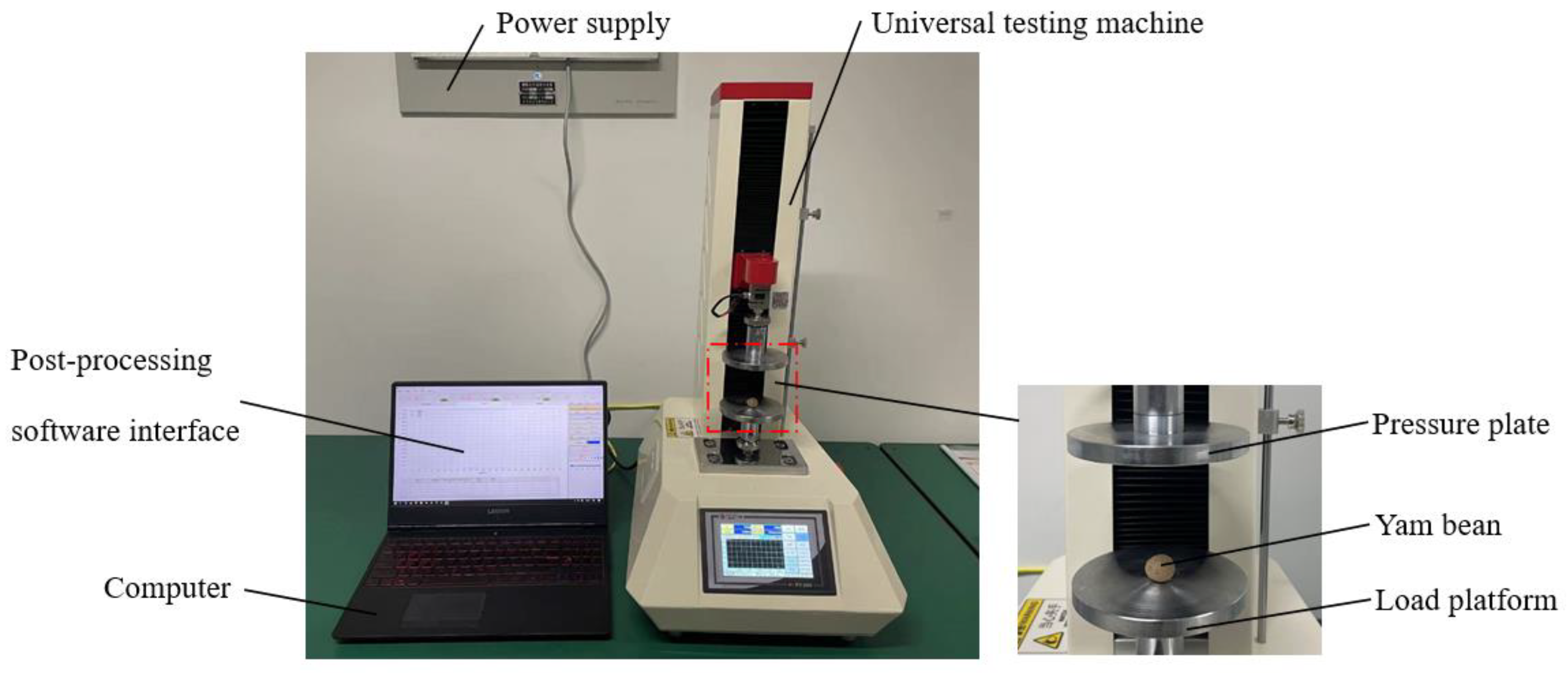
2.1.2. Determination of Shear Modulus and Poisson’s Ratio

The thin skin and small size of yam bean seeds make compression by the traditional cylindrical method more difficult. After the pre-test exploration, 10 yam beans were selected as the test material, which could ensure the validity of the test data, as well as the high efficiency of the test [22]. The uniaxial compression test of yam beans was carried out by using a universal testing machine (Pu Yan, PY-880, Dongguan, China) with 0.5% accuracy, as shown in Figure 1.

The uniaxial compression test method was referenced from the Method for Determination of Physical Properties of Grain and Oil Seeds [23] and previous studies in the evaluation of mechanical properties of seed materials [24]. Before the modulus of elasticity was determined, the yam bean was placed horizontally on the universal testing machine’s loading platform. The compression speed and time were set to 10 mm/min and 5 s, respectively. Compression in the thickness direction was stopped after 5 s. The load-displacement data during the compression of yam beans were obtained by using the post-processing software that comes with the universal testing machine, and the mean value was obtained through multiple repetitions of the test. The modulus of elasticity of the yam bean is calculated from Equation (1) as $E=8.71$ × 10⁷ Pa.

$$E={\displaystyle \frac{\sigma }{\epsilon }}$$

(1)

where $E$ is the modulus of elasticity of yam bean, Pa; $\sigma$ is the maximum compressive stress, Pa; $\epsilon$ is the line strain.

Prior to Poisson’s ratio determination test, the length and thickness of the yam bean were recorded. Poisson’s ratio was calculated by comparing the change in length and thickness of yam beans before and after the test. The test was conducted by placing the yam bean horizontally on the platform and applying axial compression at a rate of 0.1 mm/s. The compression was stopped when the yam bean appeared to crack. The yam bean length deformation data were recorded by a universal testing machine. The measurement of yam bean thickness deformation data was performed using digital vernier calipers. Poisson’s ratio was calculated as shown in Equation (2), and the results are averaged.

$$\mu ={\displaystyle \frac{\mathsf{\Delta }H/H_{yb}}{\mathsf{\Delta }L/L}}={\displaystyle \frac{(H_1-H_{yb})/H_{yb}}{(L_1-L)/L}}$$

(2)

where $\mu$ is Poisson’s ratio; $\mathsf{\Delta }H$ is the deformation in the thickness direction of the yam bean, mm; $H_1$ is the thickness of the yam bean after rupture, mm; $H_{yb}$ is the original thickness of the yam bean, mm; $\mathsf{\Delta }L$ is the deformation of the yam bean in length direction, mm; $L_1$ is the length of the yam bean after rupture, mm; $L$ is the original length of the yam bean, mm.

Poisson’s ratio of the yam bean was calculated to be 0.387 based on Equation (2). The shear modulus of the yam bean was calculated to be 3.14 × 10⁷ Pa according to Equation (3).

$$G={\displaystyle \frac{E}{2(1+\mu )}}$$

(3)

where $G$ is the shear modulus of the yam bean, Pa; $E$ is the elastic modulus of the yam bean, Pa; $\mu$ is Poisson’s ratio of the yam bean.

2.2. Measurement of Exposure Parameters

Machinery related to the sowing and harvesting of yam beans has rarely been studied. The exposure parameters related to yam beans cannot be obtained through the available literature and, therefore, need to be determined by physical tests. The contact parameters that need to be determined in the discrete element simulation of mechanized yam bean sowing and harvesting operations include the coefficient of static friction among yam beans, the static friction coefficient between yam bean and PE plate, the rolling friction coefficient between yam bean and yam bean, the rolling friction coefficient between yam bean and PE plate, the collision recovery coefficient between yam bean and yam bean, and the collision recovery coefficient between yam bean and PE plate. The contact parameter values obtained from physical experiments can serve as a benchmark range for discrete element simulation trials.

2.2.1. Determination of Crash Recovery Coefficient

The collision recovery coefficient is a physical quantity that measures the degree of rebound of two objects after a collision and can describe the energy loss of an object during a collision [25,26]. The coefficient of recovery of collisions between yam beans and yam peas was ascertained through the free-fall method collision method. A portion of the yam bean was made into a yam bean plate and placed horizontally. The surface of the yam bean board has no special treatment and is the original texture of the yam bean. The yam bean was dropped freely from a distance of $H=48$ cm from the yam bean plate. The yam bean bounced back after hitting the yam bean plate, and the maximum height of the bounce was determined to be $h_{\max }$ by the camera system. The above operation was repeated 10 times, and the results were calculated as an average. The test procedure is shown in Figure 2. The camera used for the test was a Canon EOS 77D (Beijing Jingdong Century Trading Co., Beijing, China), with an effective camera resolution of 24.2 million. The collision process between the yam bean and the yam bean was recorded by the camera in the form of high-speed continuous shooting, and the height of the yam bean pop-up was measured and calculated manually. The collision recovery coefficient $e$ is defined as the ratio of the relative separation velocity after the collision to the relative approach velocity prior to the impact, which is calculated as Equation (4).

$$e={\displaystyle \frac{{v_2}^{\prime }-{v_1}^{\prime }}{v_1-v_2}}$$

(4)

where ${v_1}^{\prime }$ is the speed of the yam bean after collision, m/s; ${v_2}^{\prime }$ is the speed of the yam bean plate after collision, m/s; $v_1$ is the speed of the yam bean before collision, m/s; $v_2$ is the speed of the yam bean plate before collision, m/s.

The yam bean falls freely and bounces up after a collision with the yam bean plate. Before and after the collision, only the yam bean relies on its own gravity to do work, and the yam bean plate does not move. Therefore, the velocity of the yam bean plate before and after the collision is 0. ${v_1}^{\prime }=\sqrt{2g{h}_{\max }}$, $v_1=\sqrt{2gH}$ ($g$ is the acceleration of gravity, m/s²). Equation (4), for calculating the collision recovery factor, can be simplified to Equation (5).

$$e=\sqrt{{\displaystyle \frac{h_{\max }}{H}}}$$

(5)

The test results, etc., were brought into Equation (5) to obtain a collision recovery coefficient of 0.46 between yam bean and yam bean. The yam bean plates were replaced with PE plates and the above test procedure was repeated. The collision recovery coefficient between the yam bean and the PE plate was 0.51.

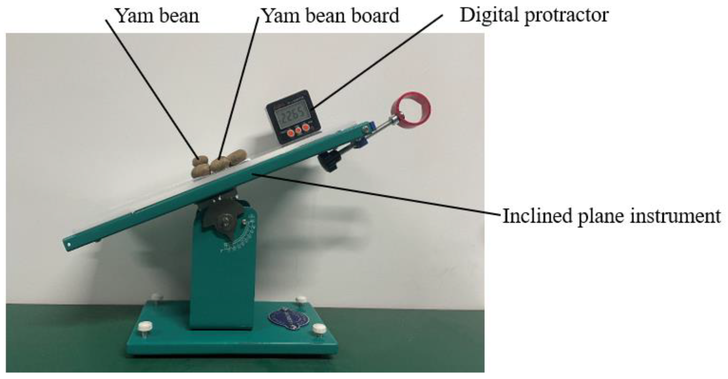
2.2.2. Determination of the Coefficient of Friction

The coefficient of static friction of the yam bean was determined using the inclined plane method with the measuring equipment shown in Figure 3. Slope adjustment is manually controlled by slowly pushing the end of the inclinometer during the test. To measure the coefficient of static friction between the yam bean and the yam bean, attach the bottom of the yam bean to the platform using bonding adhesive to form a yam bean plate, with the yam beans close together. Place the yam bean plate on the test plane of the inclinometer and place the yam bean on the yam bean plate. Slowly turn the plane of the inclinometer test counterclockwise. Stop turning the plane of the inclinometer test when a single yam bean slides on the yam bean plate. Record the angle shown by the digital protractor (accuracy of 0.01°) at this point as the ${\phi }_1$ angle of sliding friction between the yam bean and the yam bean. The coefficient of static friction $f_1$ is calculated as Equation (6).

$$f_1=\tan {\phi }_1$$

(6)

Twenty yam beans were randomly selected for static friction coefficient determination, and the test results were averaged. For static friction coefficient determination, the yam bean plate was placed longitudinally on the platform and the yam beans were placed in the same direction on the yam bean plate. The coefficient of static friction between yam bean and yam bean was measured to be 0.41. To determine the coefficient of static friction between the yam bean and PE plate, the yam bean plate was replaced with a PE plate placed on the test plane of the inclinometer. Place the yam beans on a PE plate. Determination was carried out according to the method for determining the coefficient of static friction between yam bean and yam bean. The coefficient of static friction between yam bean and PE plate was obtained as 0.24.

The coefficient of rolling friction is determined with reference to the coefficient of static friction. The yam bean board is placed horizontally on the platform and the yam beans are placed in the same direction on the board. When a single yam bean roll occurs on the yam bean plate, stop turning the inclinometer to test the plane. Record the angle displayed by the digital protractor at this point as the angle of rolling friction between the yam bean and the yam bean. The rolling friction coefficient $f_2$ is calculated as in Equation (7).

$$f_2=\tan {\phi }_2$$

(7)

Twenty yam beans were randomly selected for rolling friction coefficient determination, and the test results were averaged. The coefficient of rolling friction between yam bean and yam bean was measured to be 0.17. Similarly, the coefficient of rolling friction between the yam bean and the PE plate was measured to be 0.09.

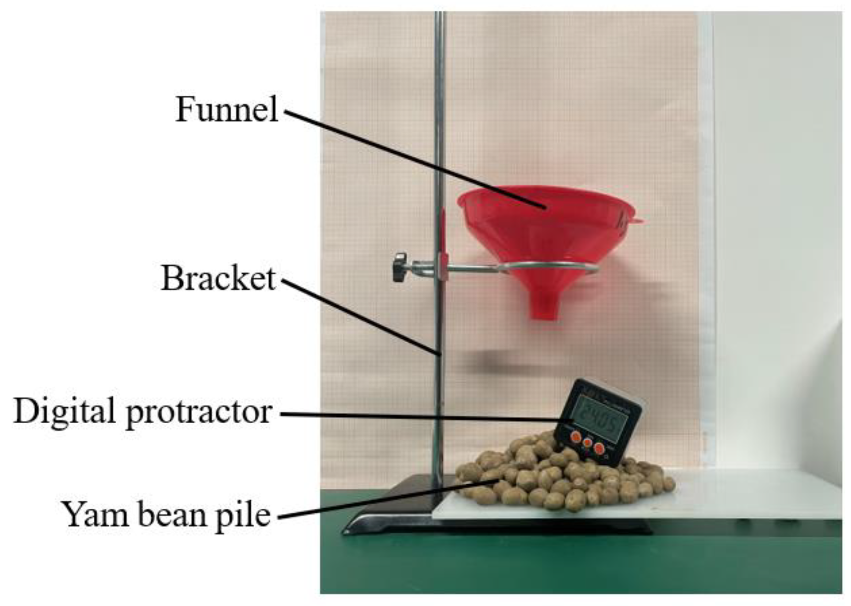
2.3. Angle of Repose Determination

The angle of repose was determined through experimentation conducted on a custom-fabricated test apparatus. The yam bean was placed in a funnel to allow it to fall freely and form an angle of repose, as shown in Figure 4. When the yam bean is entirely at rest, a mound of material will be formed, and the angle of the mound will be measured as the angle of repose. The test was repeated five times, and the angle of repose of the yam bean grain was determined to be 24.85 degrees by calculating the average of the test results.

2.4. Establishment of Discrete Element Simulation Model

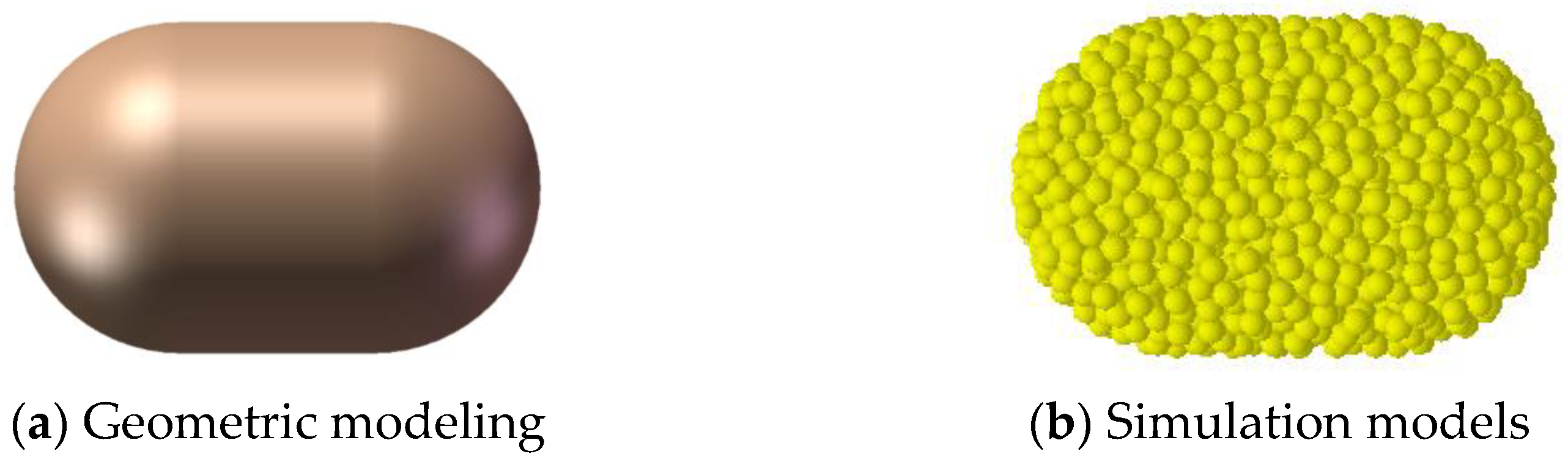
2.4.1. Yam Bean Simulation Model Establishment

Based on the determined three-axis dimensions and shape characteristics of the yam bean, through the application of the 3D modeling software Solidworks (Version: 2022), a geometric model of the yam bean was successfully established. The geometric model of the yam bean was imported into the discrete element simulation software EDEM for particle filling. For the purpose of improving the accuracy of the simulation model, particle stacking was used to set up the simulation model of the yam bean, and the geometric model and simulation model of the yam bean are shown in Figure 5.

2.4.2. Discrete Element Simulation Parameter Setting

The EDEM simulation test process was carried out by filling the yam bean simulation model using the particle filling method, and the particles were chosen from the Hertz–Mindlin model [27]. The yam bean angle of the repose simulation determination model was modeled based on the funnel of an actual physical angle of the repose determination test. The yam bean particles were generated by constructing a virtual particle plane on the upper surface of the funnel at a rate of 200/s, and the dimensions of the generated particles were set to a constant value. The simulation test was conducted over a total duration of 3 min, with the time step configured as 20% of the relevant parameter.

2.5. Yam Bean Discrete Element Parameter Calibration

Relying on the physical and contact parameters relevant to yam beans that were determined in the preceding part, the Plackett–Burman test took the simulated static angle as the response value [28]. The parameters of the simulation test were checked for relevance. The optimal range of intervals for the significance parameters was finally determined by the steepest climb test. Based on the data from the Central Composite Design tests, a quadratic regression model was formulated to describe the relationship between the separate significant parameters and the response values. The relative error between the angle of repose of the physical experiment and that of the simulation experiment was adopted as the response value.

2.5.1. Plackett–Burman Test

Plackett–Burman test parameter ranges are physical test measurements. The response value was defined as the angle of repose of the yam bean simulation test, and parameters significantly influencing this response value were selected through the Plackett–Burman test. The extreme values (minimum and maximum) of the test parameters included in

Table 1. Plackett–Burman test parameter table.

NO.	Test Parameters	Encodings
		Low (−1)	Middle (0)	High (+1)
X1	Yam bean Poisson’s ratio	0.252	0.387	0.522
X2	Yam bean shear modulus (Pa)	2.14 × 107	3.14 × 107	4.14 × 107
X3	Collision recovery coefficient between yam bean and yam bean	0.36	0.46	0.56
X4	Collision recovery coefficient between yam bean and PE plate	0.41	0.51	0.61
X5	Coefficient of static friction between yam bean and yam bean	0.31	0.41	0.51
X6	Coefficient of static friction between yam bean and PE plate	0.14	0.24	0.34
X7	Rolling friction coefficient between yam bean and yam bean	0.07	0.17	0.27
X8	Rolling friction coefficient between yam bean and PE plate	0.03	0.09	0.15

were coded as −1 and +1, respectively, with the coded value −1 reflecting a low level of the parameter and +1 representing a high level of the parameter.

2.5.2. Steepest Climb Test

Relying on the results of the Plackett–Burman test, the steepest climb test was carried out on the significant parameters that had been screened. The relative deviation of the angle of repose between the simulation test and the physical test was adopted as an assessment indicator to define the proper range of parameter values for the simulation test. All other non-significant parameters were used as parameter values throughout the simulation testing, using the average values established from the actual experiments. That is, Poisson’s ratio of the yam bean is 0.387, the shear modulus of the yam bean is 3.14 × 10⁷, the coefficient of recovery of the collision between the yam bean and the yam bean is 0.46, the coefficient of recovery of the crash between the yam bean and the PE plate is 0.51, and the coefficient of rolling friction between the yam bean and the PE plate is 0.09.

2.5.3. Central Composite Design Test

The optimal range intervals of values for the parameters playing a decisive role in yam bean simulation tests were obtained via the Plackett–Burman test and the steepest climb test. The Central Composite Design experimental design for significant parameters took the relative error of the angle of repose between the simulation test and the physical test as the testing criterion. The coding of different levels for the simulation parameters of yam beans is presented in

Table 2. Level coding table of parameters.

Levels	Parameter
	X5	X6	X7
−1.682	0.363	0.193	0.123
−1	0.39	0.22	0.15
0	0.43	0.26	0.19
+1	0.47	0.30	0.23
+1.682	0.497	0.327	0.257

.

2.6. Regression Fitting Modeling Based on Machine Learning Algorithms

A neural network is a computational model that takes input data and transforms them through multiple layers of nonlinear transformations by mimicking the way biological neurons work, ultimately leading to a prediction. The neural network model in structural form mainly comprises input layers, hidden layers, output layers, and neuron connections between layers, as shown in Figure 6. The core idea of a neural network is to make the output of the neural network as close to the true value as possible by adjusting the parameters in the network, i.e., weights and biases. The main working processes of neural network models are forward propagation, loss calculation, back propagation, and iterative optimization. It has a remarkable ability for nonlinear mapping, as well as self-learning and self-adaptive characteristics, making it appropriate for the predictive treatment of data. This paper is modeled for discrete element parameter calibration, which is a small sample project. There is a complex nonlinear coupling between the discrete element parameters and the angle of repose, which is difficult to be accurately modeled by traditional linear regression methods. The BP neural network has a strong function approximation ability, and GA-BP and PSO-BP optimize the initial parameters of the network by genetic algorithm and particle swarm algorithm, which can overcome the defects of the BP neural network that are easy to fall into the local optimum. These three models, which are able to fully explore the data features under limited data, are more advantageous than the traditional statistical models. At the same time, in order to solve the problem of insufficient data, the original data and the inverse normalization process monitor the validation set error to avoid the phenomenon of overfitting. There have been related scholars for a small number of datasets for machine learning algorithms for model optimization, model prediction, and validation on the basis of orthogonal test data [20,28]. The test results of Central Composite Design were separately employed as the datasets for regression fitting modeling of BP, GA-BP, and PSO-BP. The coefficient of static friction between yam bean and yam bean, the coefficient of static friction between yam bean and PE plate, and the coefficient of rolling friction between yam bean and yam bean were the predictor variables. The relative error between the angle of repose of the yam bean simulation test and the angle of repose of the physical test was the target variable. The dataset of 23 groups was randomly partitioned into 18 (80%) for model training and 5 (20%) for testing and validation.

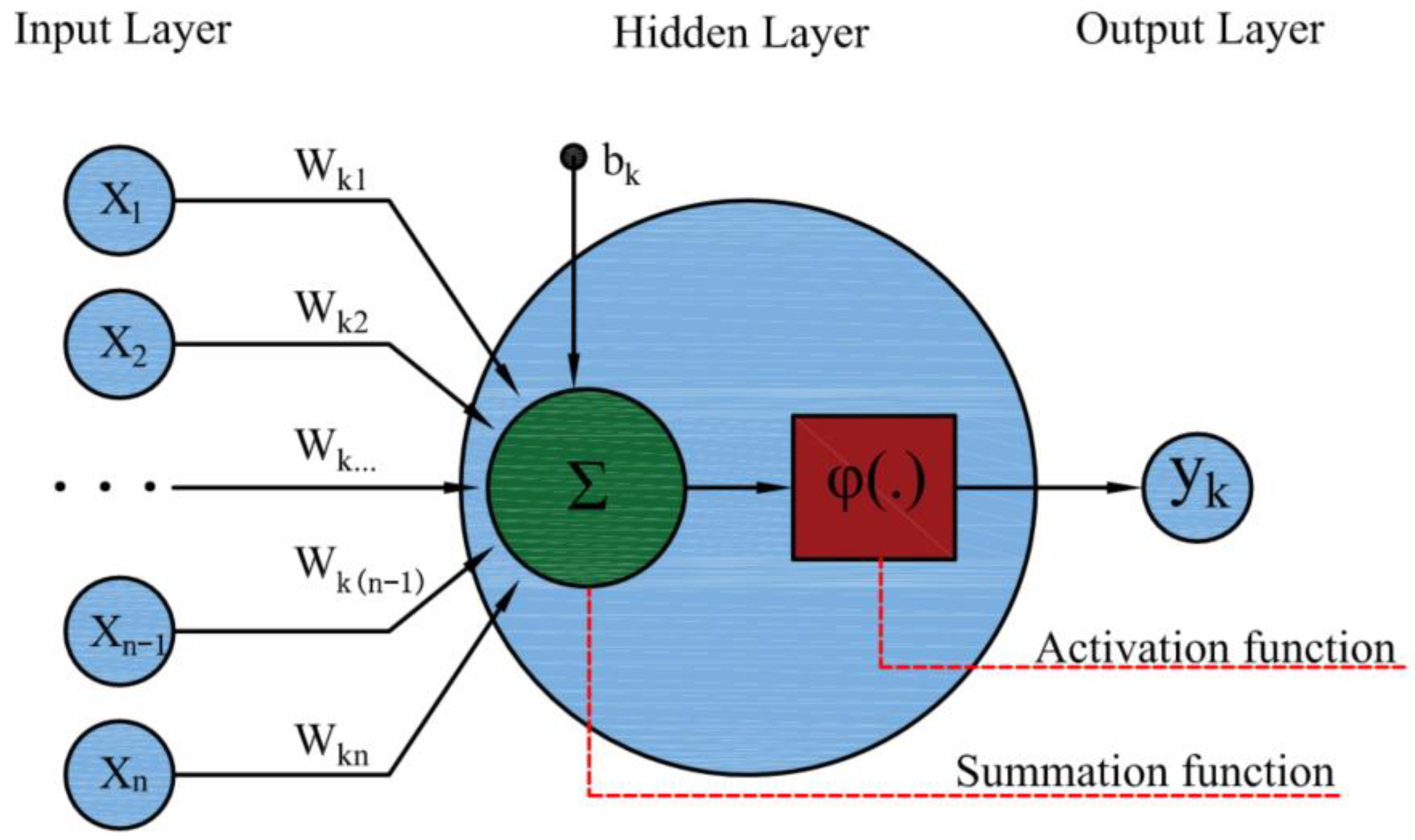
2.6.1. BP Model Building and Training

For the BP neural network model, prior data preprocessing and dataset splitting are essential steps to enhance the training efficiency. The input feature set comes to be the coefficient of static friction between yam bean and yam bean, the coefficient of static friction between yam bean and PE plate, and the coefficient of rolling friction between yam bean and yam bean. The topology design is also performed to initialize the weights and threshold lengths. The training outcomes are processed as fitness values for selection, crossover, and mutation. The final error is determined, and modeled data forecasts are made. The BP neural network model is a three-layer structure in which the hidden layer is set as a single layer and the number of nodes in the hidden layer is seven. The tansig function is used for the implicit layer functions and the purelin function is used for the output layer. The data are normalized using the mapminmax function. Initial weights and thresholds are automatically assigned randomly. The regularization type is set to L2 regularization. For hyperparameter tuning, the target error range is set to 0.01–0.0001, the learning rate range to 0.1–0.001, and the maximum training steps range to 10–1000. The final target error is set to 0.001, the learning rate is set to 0.01, and the maximum number of training steps is 100.

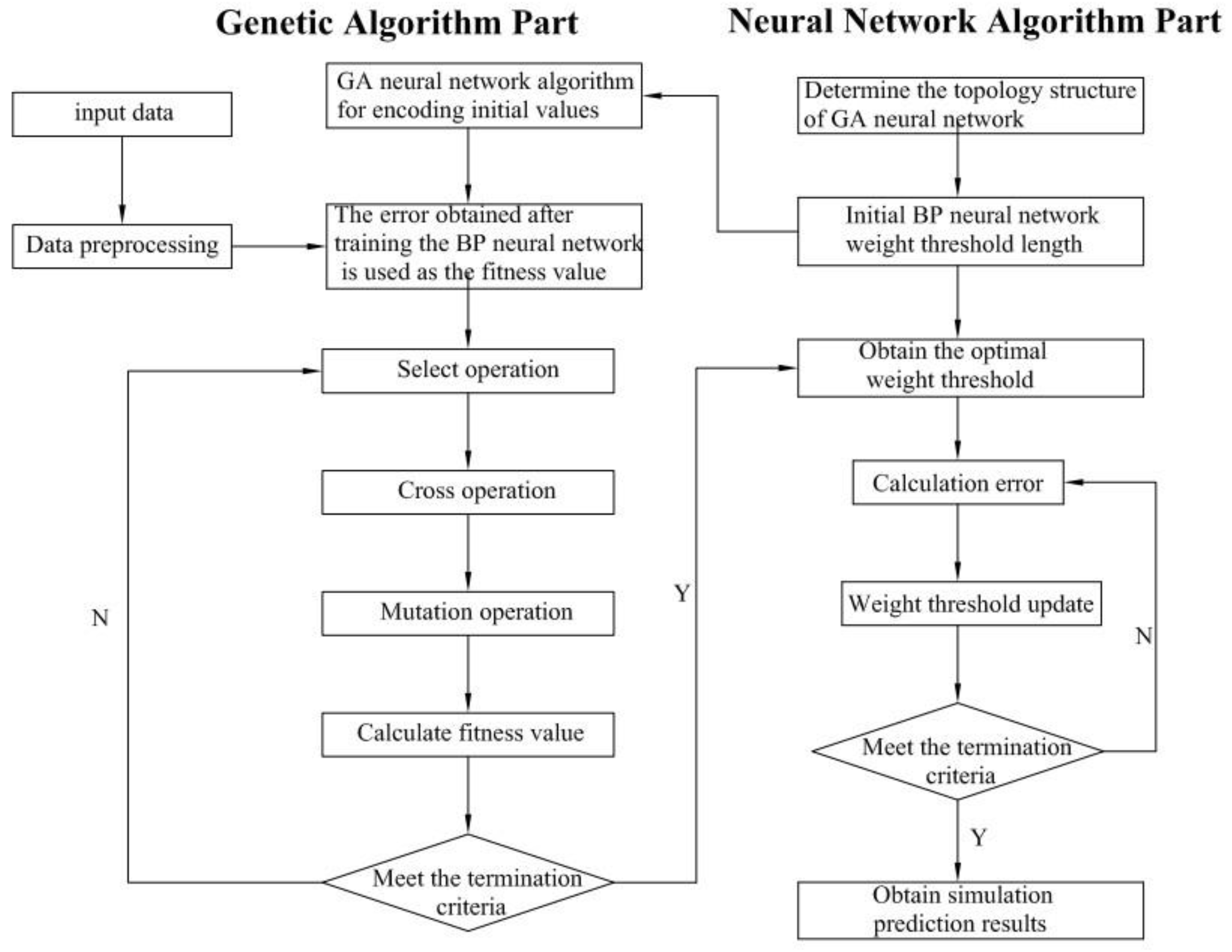
2.6.2. GA-BP Model Construction and Training

The GA-BP neural network optimization model takes full advantage of the global search capabilities of the genetic algorithm to optimize the initial weights and biases of the BP neural network algorithm. This optimization arrangement prevents the BP neural network from falling into a local optimum. It enhances the performance of the model in terms of stability, accuracy, etc., as well as improving the convergence speed and the generalization capacity of the model. The optimization procedure of GA-BP comprises decoding the ideal individual obtained using a genetic algorithm to obtain a set of optimized weights and thresholds. Subsequently, the data are introduced into a BP neural network, and the training set is utilized to train the BP neural network that has been equipped with the most suitable weights and thresholds. The output is determined by forward propagation, the error is calculated, and then the weights and thresholds are changed via back propagation so that the error is constantly reduced. The execution of the genetic algorithm and the training process of the BP neural network are repeated several times to fulfill the termination condition, and the GA-BP algorithm flowchart is shown in Figure 7. GA-BP sets the population size to 120, the number of iterations to 150, the crossover coefficient to 0.8, and the coefficient of variation to 0.2. The chromosome coding format is encoded in real numbers and the fitness function is the gabpEval function.

2.6.3. PSO-BP Model Construction and Training

The PSO-BP neural network optimization model integrates particle swarm population intelligence search. Its ability to start from many initial points avoids searching solely in localized areas. It raises the likelihood of finding a globally optimal solution and improves the generalization ability and the accuracy of predictions made by the model. As the program advances, the PSO-BP algorithm normalizes data to determine the globally optimal particles after multiple rounds of repetitions. Their matching weights and thresholds are the optimized parameters. The weights and thresholds that have undergone optimization are incorporated into a BP neural network and trained with the data from the training set. The output is determined by forward propagation, the error is calculated, and then the weights and thresholds are changed via back propagation to reduce the error further. In the PSO-BP algorithm, the particle swarm size is set at 50, the inertia weight is 0.4, both learning factors are taken as 2, and the maximum number of iterations is set to 120.

3. Results and Discussion

3.1. Analysis of Plackett–Burman Test Results

The simulated angle of repose test of yam beans on PE plates is influenced by numerous factors. Hence, it is essential to conduct a Plackett–Burman test to determine the significance of each factor’s impact on this specific test. Taking the rest angle of the yam bean simulation test as the response value, the parameters for the yam bean rest angle simulation test were screened. A total of 12 test sets were executed, with each set repeated three times to calculate the average value. The experimental methods and results are recorded in

Table 3. Plackett–Burman test protocol and results.

No.	Parametric								Repose Angle θ/(°)
	X1	X2	X3	X4	X5	X6	X7	X8
1	1	1	−1	1	1	1	−1	−1	29.94
2	1	1	−1	−1	−1	1	−1	1	21.10
3	1	1	1	−1	−1	−1	1	−1	25.68
4	−1	1	1	−1	1	1	1	−1	32.62
5	1	−1	−1	−1	1	−1	1	1	31.45
6	−1	−1	−1	−1	−1	−1	−1	−1	21.52
7	−1	1	1	1	−1	−1	−1	1	22.11
8	1	−1	1	1	1	−1	−1	−1	24.97
9	−1	1	−1	1	1	−1	1	1	28.72
10	1	−1	1	1	−1	1	1	1	27.44
11	−1	−1	1	−1	1	1	−1	1	31.76
12	−1	−1	−1	1	−1	1	1	−1	26.35

. The significance analysis of the findings of the Plackett–Burman test is provided in

Table 4. Plackett–Burman test parameter significance analysis.

Parameters	Effect	Mean-Square Sum	Impact Rate	Order of Significance
X1	0.42	0.52	0.33	6
X2	0.28	0.24	0.15	7
X3	0.08	0.02	0.01	8
X4	−1.6	7.68	4.92	4
X5	5.04	76.31	48.84	1
X6	3.29	32.54	20.83	2
X7	2.64	20.96	13.42	3
X8	1.08	3.52	2.25	5

. From Table 4, it can be seen that the coefficient of static friction between yam bean and yam bean, the coefficient of static friction between yam bean and PE plate, and the coefficient of rolling friction between yam bean and yam bean have a significant effect on the angle of repose of the simulation test. Other simulation test settings have a limited impact on the simulation test rest angle. Therefore, it is necessary to analyze further the law of influence of the coefficient of static friction between yam bean and yam bean, the coefficient of static friction between yam bean and PE plate, and the coefficient of rolling friction between yam bean and yam bean on the relative error of the angle of repose of the yam bean between the physical test and the simulation test.

The design proposal and findings of the steepest climb test are depicted in

Table 5. Steepest climbing test design scheme.

No.	Parametric			Repose Angle θ/(°)	Relative Error Y/%
	X5	X6	X7
1	0.31	0.14	0.07	20.57	17.22%
2	0.35	0.18	0.11	22.16	10.83.%
3	0.39	0.22	0.15	24.09	3.05%
4	0.43	0.26	0.19	25.39	2.17%
5	0.47	0.30	0.23	27.04	8.81%
6	0.51	0.34	0.27	30.20	21.54%

. As the static friction coefficient between yam bean and yam bean, the rolling friction coefficient between yam bean and yam bean, and the static friction coefficient between yam bean and PE plate increase, the relative error between the simulated angle of repose of the yam bean and the physical angle of repose shows a tendency to increase firstly and then decrease. The trend may be derived from the threshold effect of inter-particle friction. The higher the coefficient of friction, the higher the inter-particle friction. However, the particles are too tightly packed when the friction is too high, deviating from the actual loose packing state. The fourth group of tests had the smallest relative error. The test levels of Group 4 were selected as the central point for the Central Composite Design experiment, with optimal range intervals of 0.39–0.47, 0.22–0.30, and 0.15–0.23 for X₅, X₆, and X₇.

The scheme and results of the Central Composite Design test are documented in

Table 6. Central Composite Design experiment design scheme and results.

No.	Parametric			Relative Error Y/%
	X5	X6	X7
1	1	1	−1	0.77
2	1	1	1	7.29
3	0	0	0	3.15
4	1.682	0	0	2.82
5	−1	−1	−1	8.24
6	−1	1	−1	3.65
7	0	1.682	0	2.67
8	0	0	0	2.38
9	1	−1	−1	2.33
10	−1	1	1	5.17
11	0	0	1.682	6.13
12	0	0	0	1.47
13	0	0	0	1.93
14	0	0	0	2.86
15	−1.682	0	0	6.73
16	−1	−1	1	8.61
17	0	0	0	2.06
18	0	−1.682	0	6.28
19	0	0	0	2.11
20	0	0	−1.682	2.94
21	0	0	0	2.93
22	0	0	0	3.30
23	1	−1	1	4.85

. The analysis of variance (ANOVA) of the relative error test results of the yam bean rest angle using Design-Expert13 software yielded a quadratic polynomial regression equation of Equation (8):

Y = 2.46 − 1.25A − 0.9681B + 1.19C + 1.11AB + 0.8938AC + 0.6438BC +
0.8973A² + 0.7912B² + 0.8124C²

(8)

The results of the Central Composite Design test regression model variance are shown in

Table 7. Variation analysis of Central Composite Design test quadratic model.

Source of Variance	Mean Square	Degree of Freedom	Sum of Square	p-Value
Model	105.82	9	11.76	<0.0001 **
X5	21.18	1	21.18	<0.0001 **
X6	12.80	1	12.80	<0.0001 **
X7	19.44	1	19.44	<0.0001 **
X5X6	9.92	1	9.92	0.0003 **
X5X7	6.39	1	6.39	0.0017 **
X6X7	3.32	1	3.32	0.0141 **
X52	12.79	1	12.79	<0.0001 **
X62	9.95	1	9.95	0.0003 **
X72	10.49	1	10.49	0.0002 **
Residual	5.36	13	0.4126
Lost proposal	2.25	5	0.4504	0.4057
Pure error	3.11	8	0.3890
Aggregate	111.19	22

Note: ** in Table 7 indicates that the impact is extremely significant (p < 0.01).

. Based on Table 7, it can be concluded that the effect of factors X₅, X₆, X₇ and their interaction terms X₅X₆, X₅X₇, X₆X₇, as well as the quadratic terms X₅², X₆², and X₇² on the relative error of the angle of repose is extremely significant. This is in line with the theory that inter-particle contact properties dominate the stacking behavior in existing studies. For example, there is a significant relationship between the stacking angle of sesame seeds and the inter-particle friction coefficient as derived in the literature [29], which is consistent with the findings of this study. The significance test on the angle of repose regression model indicated a p-value of less than 0.0001, confirming a strongly significant relationship between the angle of repose and the regression equation. The p-value of the misfit term is 0.4057, which is greater than 0.05, indicating that the model fits well without misfit. The coefficient of determination R² of the regression equation is 0.9518 and the corrected coefficient of determination adjusted R² is 0.9184, both of which are close to 1, further indicating that the model has a good fit. Overall, the regression model is significantly valid, effectively mirrors the actual conditions, and can be applied to forecast and analyze the angle of repose in future studies.

3.2. Machine Learning Regression Model Analysis

3.2.1. Model Comparison

The test data from the Central Composite Design underwent regression fit modeling through the application of three algorithms. The software version used for modeling is MATLAB R2022b. Through the comparison of R², MSE, and MAE among the models, the most fitting regression model for the yam bean calibration test procedure was ascertained. The results of model comparison after multiple iterations of training of the three algorithms are shown in

Table 8. Comparison of models.

Arithmetic	R2	MSE	MAE
BP	0.9004	0.5204	0.3554
GA-BP	0.9611	0.2112	0.2809
PSO-BP	0.9485	0.2166	0.2883

.

As can be seen from the table, the comparative findings of R² of the three models are GA-BP > PSO-BP > BP. The BP algorithm is a classic error back propagation method. GA-BP is an integrated algorithm that combines a genetic algorithm with a BP neural network. PSO-BP is an integrated algorithm that combines the particle swarm optimization method with the BP neural network algorithm. In terms of algorithmic search technique, PSO-BP integrates the global searching ability of the particle swarm algorithm and the local searching capacity of the BP neural network. GA-BP combines the global search functionality inherent in genetic algorithms and the local search functionality of BP neural networks. The BP algorithm, on the other hand, relies on local search. The foregoing properties are one reason why GA-BP and PSO-BP fit better than BP. The superiority or inferiority of the three models cannot be assessed from model R² alone and needs to be further studied in conjunction with the models’ MSE and MAE values. The comparison of the model MSE of the three algorithms resulted in GA-BP < PSO-BP < BP. Comparing the mean absolute error for the three algorithmic models yielded that the result was GA-BP < PSO-BP < BP. MSE is used to demonstrate how accurately a model performs, and MAE is utilized to reflect the model’s stability. GA-BP surpasses the other two methods in both MSE and MAE measures, showing that it fits the model with both high accuracy and stability. GA-BP integrates the merits of genetic algorithms and BP neural network algorithms. This integration endows it with the ability to search for global optimal solutions and conduct local optimization, thereby explaining its superior overall performance. The MSE and MAE of PSO-BP are second to GA-BP, displaying better fitting accuracy. PSO-BP depends on population iterations to search for the global optimum, which results in a model that is less accurate than GA-BP and significantly less stable. The BP algorithm is overly dependent on local search and is prone to sliding into local optima; hence, its model accuracy and stability are relatively low. Taken together, GA-BP has the best overall performance, ensuring both precision and stability, which is consistent with the conclusion that GA-BP has advantages in handling smaller datasets, as verified in the literature [24], and is therefore selected for the next step of the study.

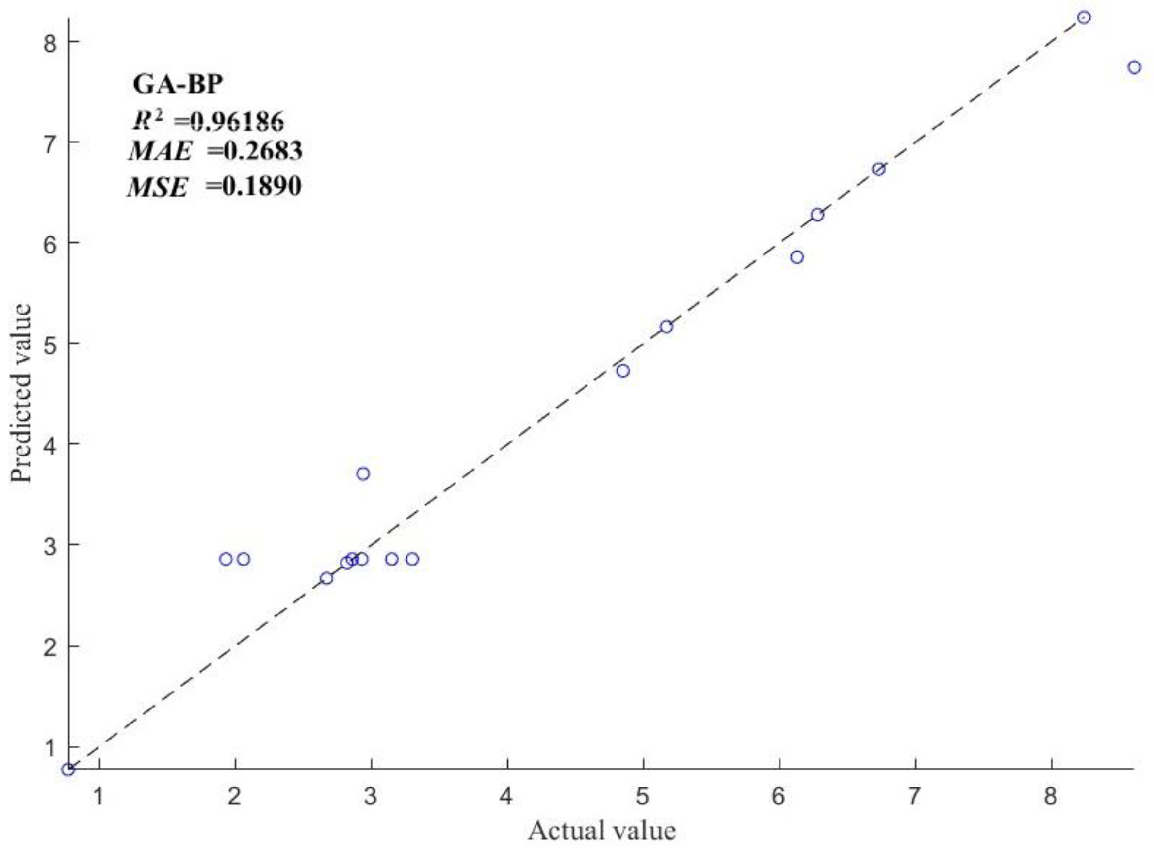
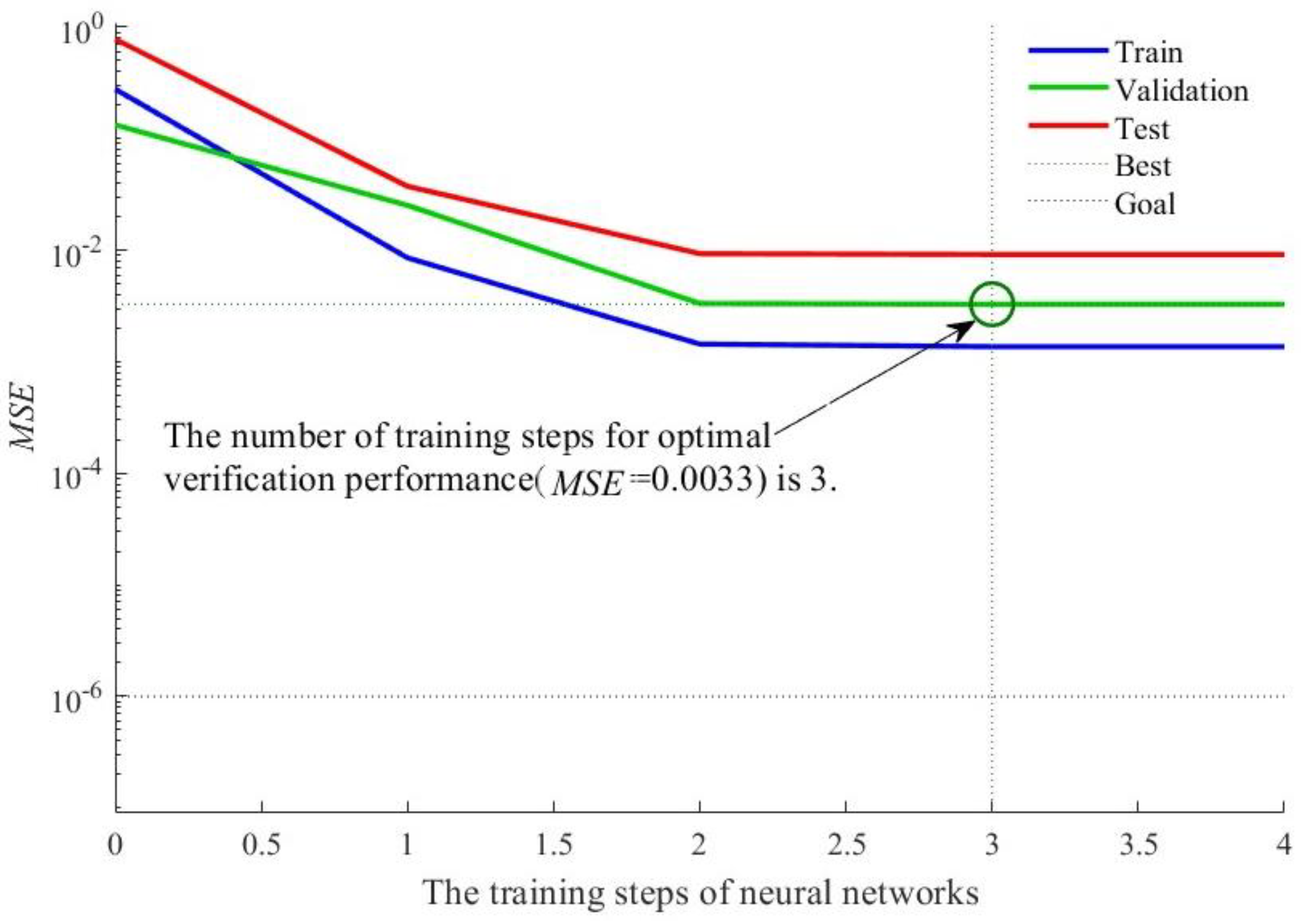
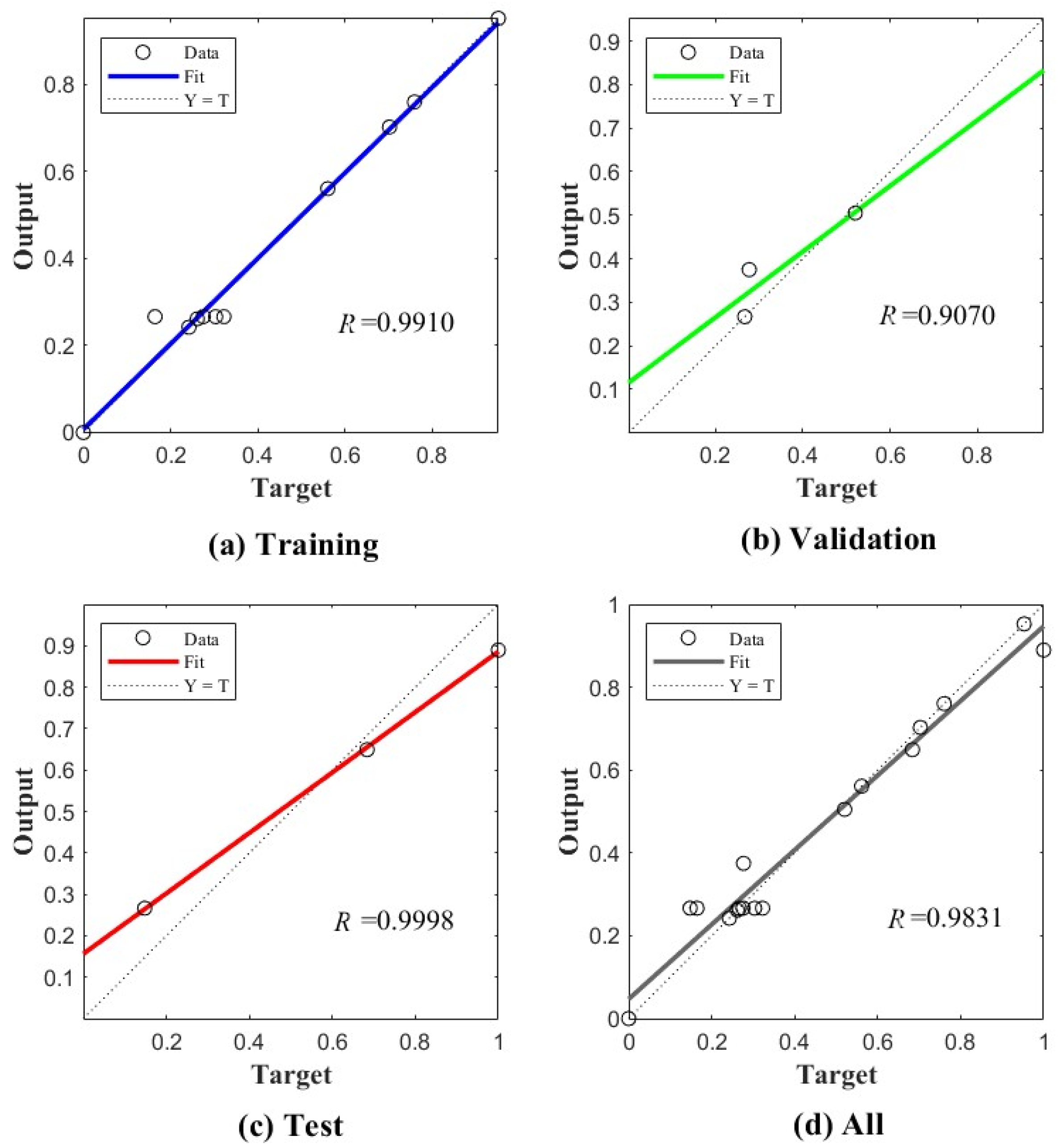
3.2.2. GA-BP Model Training Results

GA-BP combines the advantages of genetic algorithms and BP neural networks so that it can seek the global optimal solution and perform local optimization simultaneously. The R², MSE, and MAE in relation to the model are used as the assessment indexes, and the measured and predicted values of GA-BP are produced, as shown in Figure 8. The evaluation indexes of the GA-BP model are 0.9619 for the R², 0.1890 for the MSE, and 0.2683 for the MAE. In the aspects of model accuracy, stability, and fitting, it demonstrates excellent performance. The results of the study can provide a reliable modeling paradigm for subsequent discrete element-based agricultural material handling studies.

3.2.3. Model Evaluation

Regarding the chosen GA-BP, the MSE of the selected model is evaluated for performance, as shown in Figure 9. Evidently from the figure, the MSE of the model drops continuously throughout the training phase. This represents a gradual improvement in how well the model fits the training data as the training progresses. The best performance is obtained when the training reaches step 3, when the neural network training is almost complete. The foregoing analysis shows that the GA-BP training converges quickly and remains stable, indicating the feasibility of using this model in discrete element simulation experiments.

This study’s analysis of the training, validation, testing, and overall performance of GA-BP is depicted in Figure 10. The graphical results indicate that the correlation coefficients for the training, validation, testing, and combined data are 0.9910, 0.9070, 0.9998, and 0.9831, respectively. This result suggests that the model has a robust fit and good generalization ability. The correlation coefficients of the data are relatively near to each other, showing that there is no overfitting or underfitting. The application of the GA-BP algorithm has enabled this study to create a model with excellent accuracy and good generalization capabilities, which can be employed in the following experimental experiments.

3.2.4. GA-BP Optimization Test

Analysis of the machine learning regression model reveals that the GA-BP model fits the data well and provides accurate results. Loop iterations were performed using GA-BP, setting the number of model loop iterations to 150. The selection ends after the completion of the iteration and results in the individual with the closest fitness. The final results obtained were 0.476 coefficient of static friction between yam bean and yam bean, 0.289 coefficient of static friction between yam bean and PE plate, and 0.161 coefficient of rolling friction between yam bean and yam bean. The simulation of the yam bean’s angle of repose is carried out with GA-BP optimal parameter combinations. The simulated angle of repose was obtained to be 25.15° with an error value of 1.22% from the physical test, which proved the correctness of the discrete element simulation model of the yam bean based on the GA-BP neural network method. The findings of the optimization experiments show that the yam bean model and parameters created in this study can be used to follow discrete element simulation tests.

3.3. Analysis and Discussion of Test Results

When dealing with the optimization problem of discrete element calibration parameters, compared with the traditional regression analysis method, this study, by adopting the GA-BP model for data analysis and processing, combined with a series of physical tests and simulation experiments, can more accurately tap the complex nonlinear relationship between each parameter and the rest angle of the yam bean, although it is necessary to carry out several iterative calculations in the process of parameter optimization, which is important for the discrete element related to the yam bean, as it is of great significance to improve the accuracy of simulation calibration [30]. In the application field, there are fewer studies on the parameter calibration of discrete elemental simulation of the yam bean, especially lacking an accurate grasp of the complex relationship under the combined effect of multiple parameters. In this study, three different neural network models were compared with the traditional analytical method of central combinatorial tests, and the GA-BP model was applied to calibrate the parameters of discrete element simulation of the yam bean. The experimental results are consistent with those of Ma et al. and show that neural network algorithms can be used for discrete meta-parameter calibration of seeds more accurately [28,31]. This study not only provides a more reliable parameter calibration method for discrete element simulation of yam beans, but also provides new ideas and references for other similar particulate materials in terms of parameter calibration for discrete element simulation. This study is conducive to promoting the further application and development of discrete element simulation in areas such as agricultural material handling, and is potentially oriented towards future research in this area and the accurate simulation of granular material behavior in practical production applications.

In a general sense, machine learning algorithms need to have a large amount of data to ensure the accuracy of the model. The center composite test has strong sample coverage, and can cover the center point, axial point, and star point of the parameter space with a small number of samples, although the amount of data is small, but its spatial filler and orthogonality can provide better quality samples for machine learning algorithm model training. In this paper, the central composite test data are used as the dataset, and the model is optimized by machine learning algorithm, and the accuracy of the model is verified through the test. However, due to the large variability of various types of seeds, the advantages and disadvantages of using a small amount of sample data for model optimization of machine learning algorithms need to be further verified, and subsequent validation experiments with different categories of seeds need to be carried out.

4. Conclusions

(1)

By means of physical testing, the intrinsic and contact characteristics of yam beans were measured. The coefficient of static friction between yam bean and yam bean was obtained as 0.41, the coefficient of static friction between yam bean and PE plate as 0.24, the coefficient of rolling friction between yam bean and yam bean as 0.17, the coefficient of rolling friction between yam bean and PE plate as 0.09, the coefficient of recovery from collision between yam bean and yam bean as 0.46 and the coefficient of recovery from collision between yam bean and PE plate as 0.51.

(2)

A physical determination test was carried out on the angle of repose of the yam bean, and the physical angle of repose of the yam bean was obtained at 24.85°. The angle of repose calculations were carried out based on parameters acquired from physical experiments. The simulation parameters were tested for significance by the Plackett–Burman test, and it was obtained that the coefficient of static friction between yam bean and yam bean, the coefficient of static friction between yam bean and PE plate, and the rolling friction coefficient between yam bean and yam bean had a significant effect on the resting angle of the yam bean. The steepest climb test was conducted for the screened significance parameters, and the optimum ranges of values for the coefficient of static friction between yam bean and yam bean, the coefficient of static friction between yam bean and PE plate, and the rolling friction coefficient between yam bean and yam bean were determined to be 0.39–0.47, 0.22–0.30, and 0.15–0.23, using the relative error between the rest angle of the yam bean simulation test and the rest angle of the physical test as the response value. Central Composite Design experiments were conducted employing optimal parameter combinations.

(3)

The coefficient of determination (R²), mean absolute error (MSE), and mean square error (MAE) of three machine learning regression models, back propagation (BP), genetic algorithm back propagation (GA-BP), and particle swarm optimization back propagation (PSO-BP), were compared using the results of the Central Composite Design trial as a dataset. The results show that the GA-BP model performs better in terms of fitting effectiveness, stability, and accuracy. The GA-BP prediction model was analyzed and evaluated. The optimal parameter combinations were finally obtained as 0.476 static friction coefficient between yam bean and yam bean, 0.289 static friction coefficient between yam bean and PE plate, and 0.161 rolling friction coefficient between yam bean and yam bean. The test verified the accuracy of the GA-BP prediction model, and the error between the rest angle of the simulation test and the rest angle of the physical test was 1.22%.

References

1. Tamás, K. Modelling the interaction of soil with a passively-vibrating sweep using the discrete element method. Biosyst. Eng. 2024, 245, 199–222. [Google Scholar] [CrossRef]
2. Fu, J.; Zheng, Y.; Liu, F.; Zhang, J.; Fu, Q. Development and performance analysis of a rotary soil-taking punching device for improving transplanting hole structure in high-speed punching. Comput. Electron. Agric. 2024, 225, 109279. [Google Scholar] [CrossRef]
3. Mao, Z.; Cai, Y.; Guo, M.; Ma, Z.; Xu, L.; Li, X.; Hu, B. Seed Trajectory Control and Experimental Validation of the Limited Gear-Shaped Side Space of a High-Speed Cotton Precision Dibbler. Agriculture 2024, 14, 717. [Google Scholar] [CrossRef]
4. Wang, X.; Zhou, Z.; Chen, B.; Zhong, J.; Fan, X.; Andrew, H. Distribution uniformity improvement methods of a large discharge rate disc spreader for UAV fertilizer application. Comput. Electron. Agric. 2024, 220, 108928. [Google Scholar]
5. Zhou, L.; Lan, Y.; Yu, J.; Wang, Y.; Yan, D.; Sun, K.; Wang, W.; Chen, Y. Validation and calibration of soil parameters based on EEPA contact model. Comput. Part. Mech. 2023, 10, 1295–1307. [Google Scholar] [CrossRef]
6. Salma, A.N.; KuZilati, K.; Lau, K.; Shafirah, S. Material characterization and inter/intra-particle validation for DEM simulation of urea coating process. Particuology 2024, 88, 32–48. [Google Scholar]
7. Li, S.; Diao, P.; Miao, H.; Zhao, Y.; Li, X.; Zhao, H. Modeling the fracture process of wheat straw using a discrete element approach. Powder Technol. 2024, 440, 119762. [Google Scholar] [CrossRef]
8. Liang, Z.; Huang, Y.; Li, D.; Million, E. Parameter determination of a viscoelastic-plastic contact model for potatoes during transient collisions. Biosyst. Eng. 2023, 234, 156–171. [Google Scholar] [CrossRef]
9. Xu, J.; Sun, S.; Li, X.; Zeng, Z.; Han, C.; Tang, T.; Wu, W. Research on the Population Flow and Mixing Characteristics of Pelleted Vegetable Seeds Based on the Bonded-Particle Model. Agriculture 2024, 14, 752. [Google Scholar] [CrossRef]
10. Wan, L.; Li, Y.; Song, J.; Ma, X.; Dong, X.; Zhang, C.; Song, J. Vibration Response of Soil under Low-Frequency Vibration Using the Discrete Element Method. Agriculture 2023, 13, 1958. [Google Scholar] [CrossRef]
11. Duan, J.; Liu, D.; Xie, F.; Zhang, Y.; Zheng, P. Breakage simulations and experiments of granular fertilisers for optimizing a device of side-deep fertilisation by using the discrete element method. Biosyst. Eng. 2024, 238, 105–114. [Google Scholar] [CrossRef]
12. Zhu, A.; Xu, C.; Liu, Y.; Wang, J.; Tan, X. Design and Experiment of Oblique Stubble-Cutting Side-Throwing Anti-Blocking Device for No-Tillage Seeder. Agriculture 2024, 14, 2250. [Google Scholar] [CrossRef]
13. Yan, D.; Deng, W.; Xie, S.; Liu, C.; Ren, Z.; Zhao, H.; Cai, Y.; Zhao, Z. Discrete Element-Based Simulation Analysis and Research of Potato Soil Agglomerate Fragmentation and Separation. Agric. Sci. Technol. 2023, 13, 8416. [Google Scholar] [CrossRef]
14. Fan, J.; Wang, H.; Sun, K.; Zhang, L.; Wang, L.; Zhao, J.; Yu, J. Experimental verification and simulation analysis of a multi-sphere modelling approach for wheat seed particles based on the discrete element method. Biosyst. Eng. 2024, 245, 135–151. [Google Scholar] [CrossRef]
15. Jia, X.; Zhu, J.; Guo, Y.; Huang, Y.; Gao, X.; Zhang, C. Design and test of a novel converging groove-guided seed tube for precision seeding of maize. Biosyst. Eng. 2024, 245, 36–55. [Google Scholar] [CrossRef]
16. Zhu, H.; Wu, X.; Qian, C.; Bai, L.; Ma, S.; Zhao, H.; Zhang, X.; Li, H. Design and Experimental Study of a Bi-Directional Rotating Stubble-Cutting No-Tillage Planter. Agriculture 2022, 12, 1637. [Google Scholar] [CrossRef]
17. Zhang, W.; Peng, X.; Guo, J.; Guo, H.; Cheng, S. Pyrolysis kinetic analysis and model constructions of different ranks of coal and validation by GA-BP neural networks. J. Anal. Appl. Pyrolysis 2024, 182, 106659. [Google Scholar] [CrossRef]
18. Zhu, Y.; Wu, Z.; Zhu, G.; Peng, M. Study on temperature prediction of subway tunnel fire based on improved GA-BP algorithm. J. Therm. Anal. Calorim. 2024, 11, 1–18. [Google Scholar] [CrossRef]
19. Lu, K.; Liang, J.; Liu, M.; Lu, Z.; Shi, J.; Xing, P.; Wang, L. Research on Transmission Efficiency Prediction of Heavy-Duty Tractors HMCVT Based on VMD and PSO-BP. Agriculture 2024, 14, 539. [Google Scholar] [CrossRef]
20. Wei, W.; Shang, Y.; Peng, Y.; Cong, R. Prediction Model of Sound Signal in High-Speed Milling of Wood-Plastic Composites. Materials 2022, 15, 3838. [Google Scholar] [CrossRef]
21. Li, Y.; Tian, X.; Zhao, Y.; Liu, X.; Zhou, M.; Diao, F.; Wang, W. Parameter Calibration and Experiment of Polyhedral Cottonseed Discrete Element Based on Tavares Model. Trans. Chin. Soc. Agric. Mach. 2024, 55, 124–131+220. [Google Scholar]
22. Dun, G.; Wang, L.; Ji, X.; Jiang, X.; Zhao, Y.; Guo, N. Calibration and Verification of Discrete Element Parameters of Jinxiang Purple Garlic Seeds. J. Agric. Sci. Technol. 2024, 55, 124–131+220. [Google Scholar]
23. China Standard Press. Grain and Oil Standard Compilation of Determination Methods Volume Under the Fourth Edition; China Standard Press: Beijing, China, 2018. [Google Scholar]
24. Chen, Y.; Gao, X.; Jin, X.; Ma, X.; Hu, B.; Zhang, X. Calibration and Analysis of Seeding Parameters of Cyperus esculentus Seeds Based on Discrete Element Simulation. J. Agric. Sci. Technol. 2023, 54, 58–69. [Google Scholar]
25. Guo, X.; Wang, S.; Chen, S.; Li, B.; Tang, Z.; Hu, Y. Impact of Structural Parameters on the Collision Characteristics and Coefficient of Restitution of Soybean Particles on Harvester′s Cleaning Screens. Agriculture 2024, 14, 1201. [Google Scholar] [CrossRef]
26. Cui, J.; Li, X.; Zeng, F.; Bai, H.; Zhang, Y. Parameter Calibration and Optimization of a Discrete Element Model of Plug Seedling Pots Based on a Collision Impact Force. Appl. Sci. 2023, 13, 6278. [Google Scholar] [CrossRef]
27. Liu, W.; Su, Q.; Fang, M.; Zhang, J.; Zhang, W.; Yu, Z. Parameters Calibration of Discrete Element Model for Corn Straw Cutting Based on Hertz-Mindlin with Bonding. Appl. Sci. 2023, 13, 1156. [Google Scholar] [CrossRef]
28. Ma, X.; Guo, M.; Tong, X.; Hou, Z.; Liu, H.; Ren, H. Calibration of Small-Grain Seed Parameters Based on a BP Neural Network: A Case Study with Red Clover Seeds. Agronomy 2023, 13, 2670. [Google Scholar] [CrossRef]
29. Ma, W.; Zhang, S.; Yin, X.; Chen, K.; Zhu, L. A Calibration of the Contact Parameters of a Sesbania Seed Discrete Element Model Based on RSM. Processes 2023, 11, 3381. [Google Scholar] [CrossRef]
30. Yaro, N.S.Y.; Sutanto, M.H.; Habib, N.Z.; Madzlan, N.; Aliyu, U.; Ashiru, M. Comparison of Response Surface Methodology and Artificial Neural Network approach in predicting the performance and properties of palm oil clinker fine modified asphalt mixtures. Constr. Build. Mater. 2022, 324, 126618. [Google Scholar] [CrossRef]
31. Ding, X.; Wang, B.; He, Z.; Shi, Y.; Li, K.; Cui, Y.; Yang, Q. Fast and precise DEM parameter calibration for Cucurbita ficifolia seeds. Biosyst. Eng. 2023, 236, 258–276. [Google Scholar] [CrossRef]
Figure 1. Uniaxial compression test of yam bean.
Processes 13 01537 g001
Figure 2. Crash test.
Processes 13 01537 g002
Figure 3. Static friction coefficient measurement test.
Processes 13 01537 g003
Figure 4. Physical stacking angle test.
Processes 13 01537 g004
Figure 5. Geometric and simulation models of yam bean.
Processes 13 01537 g005
Figure 6. Neuron model.
Processes 13 01537 g006
Figure 7. GA-BP optimization algorithm flow.
Processes 13 01537 g007
Figure 8. Measured versus predicted values.
Processes 13 01537 g008
Figure 9. MSE performance evaluation of the model.
Processes 13 01537 g009
Figure 10. Regression analysis.
Processes 13 01537 g010