Article

Study on the Influence of Pump Performance Curve Fitting and Seal Ring Wear on Pump Intelligent Monitoring

1
School of Energy and Mechanical Engineering, Hunan University of Humanities, Science and Technology, Loudi 417000, China
2
National Research Center of Pumps, Jiangsu University, Zhenjiang 212013, China
3
Jiangsu State Spring Pump Manufacturing Co., Ltd., Zhenjiang 212009, China
*
Author to whom correspondence should be addressed.
Processes 2025, 13(5), 1529; https://doi.org/10.3390/pr13051529
Submission received: 19 March 2025 / Revised: 7 May 2025 / Accepted: 8 May 2025 / Published: 15 May 2025
(This article belongs to the Section Process Control and Monitoring)

Abstract

:
With increasing demands for energy efficiency and environmental sustainability in pump stations, the development of digital and intelligent pump systems has become crucial. In this study, we focus on three speed ratios of pumps and propose a classification algorithm for pump performance curve fitting using the polyfit function based on the least squares principle. Software programs were developed to model and analyze pump performance curves. Additionally, the impact of seal ring clearance on pump performance and energy consumption was analyzed for pumps with specific speeds of 96.2, 185.5, and 493.3. External characteristic tests were conducted to evaluate these effects. When the clearance value of the sealing ring increases, the head and efficiency of the submersible sewage pump gradually decrease, while the shaft power of the pump presents different variation trends with an increase in the specific speed of the pump. When the specific speed is low–medium, the shaft power of the pump gradually increases. However, when the specific speed is relatively high (ns > 300), the shaft power initially decreases, then increases, and finally decreases again. For intelligent monitoring, key variables and auxiliary power parameters were identified and mathematical models (Q-P and Q-H) were established as the basis for a soft measurement system. The results show that the Q-H, Q-P, and Q-η curves are generally fitted with polynomial curves of the third~fourth order. The maximum polynomial degree without inflection points is 3, while the maximum number of inflection points is 4, the two inflection points are fitted by segmentation. The pump monitoring system can integrates with an industrial cloud platform, enabling real-time parameter display, control, alarm of functions, recording and analyzing the historical data and operation trends. This research is significant for safe operation monitoring and energy conservation in pump systems.

1. Introduction

At present, many pump station monitoring systems operate in conventional semi-automatic mode, which has the disadvantages of low measurement accuracy, poor real-time performance, and insufficient reliability. Due to the highly nonlinear characteristics and complex control tasks in the monitoring system of the pump, pump monitoring mainly describes its characteristics through technical indicators such as flow, head, shaft power, efficiency, and rotational speed. The traditional method uses flowmeters, pressure gauges, etc., to measure flow rate and pressure.
With the continuous development of the modern pump industry, the research on pump foundation theory, performance optimization, and the design of pump schemes has progressed significantly. Concurrently, intelligent monitoring technologies require iterative improvements to align with evolving industrial demands [1,2,3,4,5]. Research has aimed to develop the energy efficiency of the operation of pumping equipment in systems for monitoring the efficient operation of large-scale pumping stations in the Republic of Uzbekistan [6]. Yang et al. [7] used the motor operating current to check the characteristics of centrifugal pump operating conditions, combined with the pressure signal as an auxiliary signal. Guo et al. [8] described GSHP-based remote data monitoring MODBUS and TCP/IP protocols, enabling comprehensive performance assessment through reliable data acquisition. Niu et al. [9] monitored the operating conditions of pumps with the vibration signal as the main focus. Song et al. [10] enhanced parameter calibration based on the LAB view fitting method. Panaras G et al. [11] designed an automated control system with a modular architecture, integrating motor start–stop logic, valve control, and dynamic data processing. Chen et al. [12] established a remote monitoring system based on PLC. Parameters such as the pump speed, starting liquid level, and stopping liquid level are promptly adjusted according to the influence of astronomical and meteorological conditions for operational safety. Bian et al. [13] established an intelligent monitoring platform with real-time status tracking and historical data analytics.
The leakage flow through the seal ring clearance has always been a hot topic in research on centrifugal pumps [14,15]. As a wear-prone component, the seal ring experiences gradual clearance enlargement due to operational wear [16,17]. It is of great significance to control the leakage flow in the seal ring clearance in order to improve the efficiency of the centrifugal pump and reduce energy consumption. Lomakin [18] investigated the stresses at the seal ring clearance of a centrifugal pump and found that the stability of the pump was closely related to the size of the seal ring clearance. Ayad et al. [19] investigated the effect of seal ring clearance on a semi-open centrifugal pump and found that the pump head and efficiency are inversely proportional to the seal ring clearance. Zhou et al. [20] found that a reduction in the ring clearance could effectively enhance the head and efficiency of centrifugal pumps, and achieved a 5% efficiency. Zhao et al. [21] found that the external characteristics of the centrifugal pump with different annulus clearances are consistent with the experimental data, reporting a < 5% relative error (except for a 1.06 mm clearance). Gao et al. [22] investigated the effect of the seal ring clearance on the impeller force and pressure pulsation in the pump through calculations and experimental proofs. Zhao et al. [23] conducted a numerical calculation of the influence of the seal ring clearance on a centrifugal pump with a multi-turbulence model and increasing clearance. Chen et al. [24] investigated the influence of the seal ring on the external characteristics of the pump and the influence on the highest efficiency point of the centrifugal oil pump. To explore the influence of the front ring clearance on the normal operation and internal flow characteristics of centrifugal pumps, the reliability of numerical simulation was verified by comparing the test head with the simulated head. A comparative analysis of five front-ring clearance pumps was carried out. The results showed that enlarged clearance exacerbates backflow and induces impeller flow instability, which leads to a decrease in the head efficiency [25].
In general, current advancements in pumping station monitoring methods are oriented toward intelligent, real-time, and integrated systems. In this paper, we designed a soft measurement method based on power instead of flow. The new pump and pump station monitoring device was developed using soft measurement technology: the pump power was measured, and the algorithm realized the flow to monitor the pump. The monitoring accuracy requirements were met while maintaining cost-effectiveness.

2. Pump Test System and Characteristic Curve Fitting Method

2.1. Pump Test Object and System

In this paper, a combined theoretical and experimental analysis of the pump performance across three specific speed regimes (ns = 96.2, 185.5, and 493.3) was conducted. The investigation focused on the completion of pump external characteristic curve fitting, the establishment of a remote intelligent pump monitoring system, and the development of a pump device curve solution to explore the effect of different sealing ring clearances on the performance of the pump. Figure 1 shows three kinds of submersible pumps. Table 1 shows the specific parameters of the three kinds of submersible pumps.
The experimental pipeline system of the pump consists of a valve, a DN150 electromagnetic flowmeter, a pressure transmitter, a DN150 pressure-test pipe, two 90° elbows, a 90 cm DN150 straight pipe section, and a 300 cm DN150 straight pipe section. The system structure diagram of the experimental pipeline of submersible pumps is shown in Figure 2. The test facilities and measurement methods adhered to the measurement requirements previously described [26]. The system includes a flow control device, a data acquisition device, and a data processing device. During the experiment, the flow and pressure were measured with an electromagnetic flowmeter and pressure sensor and the shaft power was measured with a shaft power tester. Then, under the valve opening adjustment, the inlet and outlet pressure and shaft power at different flow rates were obtained for calculation.
In the pump performance test, the pump efficiency is defined as follows [27]:
η = ρ g Q H P S × 100 % ,
where η is the pump efficiency, Q is the flow rate (m3/s), H is the pump head (m), and Ps is the output power of the motor (W).
H = p o u t p i n ρ g ,
where pin is the inlet total pressure and pout is the outlet total pressure (the pin and pout units are Pa).

2.2. Characteristic Curve Fitting Method

According to the specific rotational speed Formula (3), used to calculate the specific rotational speed, due to the mixed-flow pump and axial pump characteristic curves, an inflection point will appear, so the fitting mode is divided into “centrifugal pump”, “mixed-flow pump”, and “axial pump”. “centrifugal pump”is selected for ns < 300, “mixed-flow pump” is selected for 300 ≤ ns ≤ 500, and “axial pump” is selected for ns > 500, as shown in Figure 3.
n s = 3.65 n Q H 3 / 4 ,
where n is the speed (r/min).
The first step is to select five points in the vicinity of the point and obtain the third-order approximation expression g(x) = ax3 + bx2 + cx + d by the polyfit function based on the principle of least squares, and then substitute the corrected point X into g(x) to obtain g(X correction) = y1; in the second step, the correction point X is corrected for the neighboring points 1 and 3 to obtain the equation of a straight line, and then X is substituted into y2; in the third step, (y1 + y2)/2 is substituted for the y value of the correction point, and the relative error of the two is calculated. Similarly, other points can be corrected. The data correction GUI interface is shown in Figure 4.
Part of the program is as follows:
p = polyfit(X,Y,3);% (fit five data points to a cubic curve);
x = floor(x1):0.2:ceil(x2);
y = polyval(p,x);
y11 = polyval(p,xp);% (obtain the least squares correction point values);
......
y22 = a × xp + δ;% (obtain the data value obtained by correcting two adjacent points in a straight line);
yxz = (y11 + y22)/2;% (obtain the final corrected value);
pcz = (yxz − yp)/yp;% (calculate the percentage error before and after correction).

3. Results and Discussion

3.1. Pump Performance Curve Fitting

The current common curve fitting methods include polynomial fitting and Spline interpolation fitting. Data blending occurs using polynomial data fitting, while Spline interpolation achieves sound effective smoothing. However, there are excessive parameters for this interpolation method, making it less practical for general curve fitting. At the same time, all of the measurement data are assumed to contain noise when performing curve fitting. Therefore, the final fit curve does not require passing each known data point, and the criterion for measuring the fit data is that the error of the overall data is minimal. The polyfit function addresses the computational complexity and time consumption of traditional fitting algorithms while maintaining an exceptionally high fitting accuracy [28]. The general pump test data error is obtained by the interpolation method used to obtain the correction point data. In this paper, the test data are corrected by the polyfit function method based on the least squares method and the average value of the interpolation method, which further improves the accuracy of the corrected point data.
a = P o l y f i t ( x , y , n )
In Formula (4), a represents the polynomial coefficients from the highest to lowest degree; x and y are the external characteristics of the test measured data, such as x for the flow rate and y for the head; and n indicates the polynomial degree used for fitting the flow–head curve.
When using the polynomial to apply the least squares method, high-degree polynomials (typically with degree ≥ 7) violate the fundamental principle that pump characteristic curves should have minimal inflection points [29], while first-degree polynomials (linear fitting) fail to represent the actual nonlinear behavior of pump curves. Therefore, the polynomial degree is constrained to 6 for optimal fitting.
In this paper, the Q-H and Q-P curves of the centrifugal pump are fitted with second- to sixth-degree polynomials. Since the Q-η curve of the centrifugal pump is generally flat, a fixed third-degree polynomial is employed. In the polynomial fitting process, increasing the degree of fittings can improve the fitting accuracy, but excessive polynomial degrees may lead to the Runge phenomenon [30], and care should be taken to prevent this from happening.

3.1.1. Centrifugal Pump External Characteristic Curve Fitting

In this paper, the external characteristic curve is fitted with a centrifugal pump with a rotational speed of 47.9.
Table 2 shows the external characteristic data of the centrifugal pump.
The number of Q-H curve fittings of the centrifugal pump was selected 2 to 6 times, and the polynomial fitting curve was compared as shown in Figure 5.
The Q-P curve fitting of the centrifugal pump was selected 2 to 6 times, and the polynomial fitting curve was compared as shown in Figure 6.
The Q-η curve fitting of the centrifugal pump was selected 3 times.
Table 2 shows that as the polynomial fitting order increases, the correlation coefficient approaches unity, and the root mean square, the absolute error maximum, and the relative error maximum exhibit monotonic reduction. This confirms that higher-degree polynomials achieve superior fitting accuracy.
In summary, the selection principle of the number of fittings of the centrifugal pump is the number of fitting times with the highest number of selections in 2 to 6 times the absence of the Runge phenomenon.
In order to judge the magnitude of the error in the case of different fitting times, the analysis of all the cases is shown in Table 3.
As shown in Table 2, based on the calculated correlation coefficient, root mean square, absolute error maximum, and relative error maximum, the degree of curve fitting can be judged. A correlation coefficient closer to 1 indicates a better fit. The fitting correlation coefficients > 0.999, the root mean square < 1, the maximum absolute error < 2, and the maximum relative error < 1%, confirming that the fitting curve not only achieves a high precision but also maintains minimal deviations from the original data points.
In summary, the pump Q-H curve is fitted by the cubic polynomial, the pump Q-P curve is fitted by the fourth-order polynomial, and the pump Q-η curve is fitted by the cubic polynomial.
The fitted pump performance curve is shown in Figure 7.
The formula for fitting the curve is as follows:
H = 9.496827 × 10 7 Q 3 + 3.513044 × 10 4 Q 2 0.1424137 Q + 137.3357 P = 2.42893 × 10 9 Q 4 3.80352 × 10 6 Q 3 + 0.00158785 Q 2 0.0532399 Q + 61.0879 η = 9.723 × 10 7 Q 3 0.0014816 Q 2 + 0.61676 Q + 0.42226

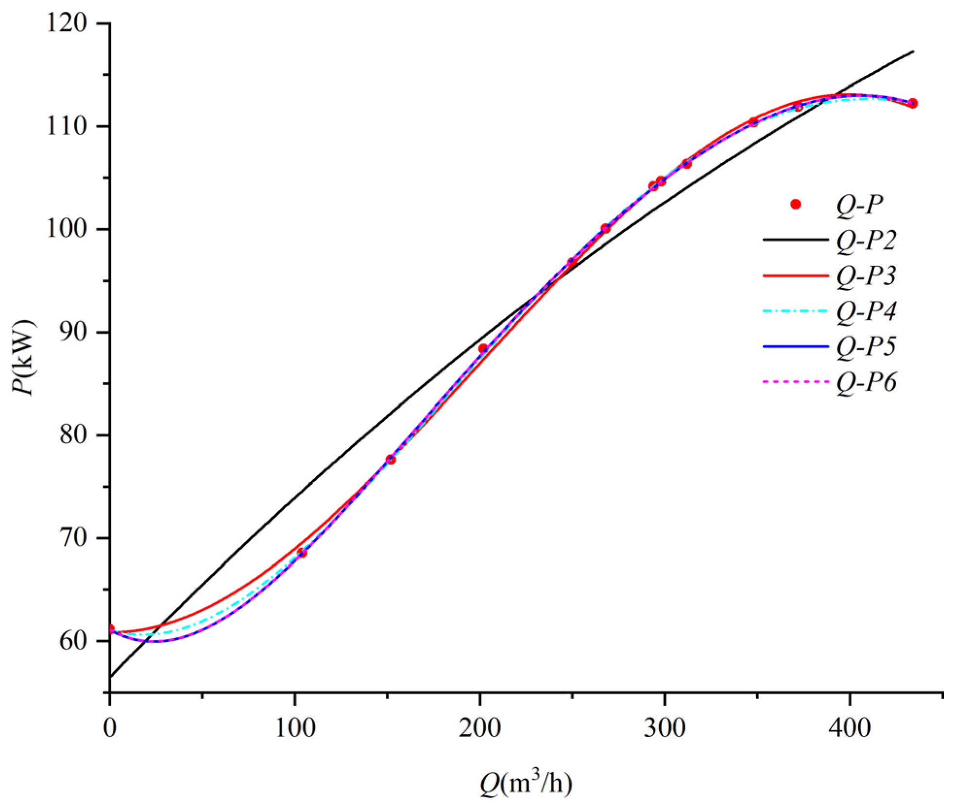
3.1.2. Axial Flow Pump External Characteristic Curve Fitting

Aiming at a situation where the external characteristic curve of the existing axial flow pump is prone to an irregular shape and it is difficult to express the actual curve behavior, a piecewise least squares polynomial fitting method is designed to connect the adjacent segmented curves using the interpolation fitting method [31,32].
The Q-H curve is partitioned into three segments: the first segment is a quadratic polynomial, and the others are cubic polynomials. The first segment is from left to right (the first segment of the Q-H curve with a negative partial derivative of Q). The second segment us from left to right (the segment where the Q-H curve has a positive partial derivative of Q). This segment is formed by interpolation fitting to connect the first and third segments. The third segment is from left to right (the second segment with a negative derivative of Q-H curve versus Q).
The Q-P curve segmentation method is consistent with the flow–head curve fitting method.
The Q-η curve is fitted with a third-degree polynomial curve, and the fitting degree is determined as above.
It can be seen from Table 4 that the pump exhibits a high fitting accuracy. The correlation coefficients of the three fitted curves exceed 0.989, the fitting errors were minimal, with the mean root square < 1, the absolute value relative error maximum < 2, and the relative error maximum < 1%. Moreover, this method not only ensures a high fitting precision but also preserves the saddle-shaped curve characteristics without introducing the Runge phenomenon, thereby validating the correctness of the fitting approach.
Key Improvements:
The formula for fitting the curve is as follows:
H = 9.14 × 10 5 Q 2 + 0.0672 Q 2.45 420.39 Q < 524.64 1.026 × 10 5 Q 3 + 0.0173 Q 2 9.75 Q + 1832   524.64 Q 586.26   4.53 × 10 8 Q 3 1.16 × 10 4 Q 2 + 0.0927 Q 15.5 586.26 < Q 999.18
P = 2.41 × 10 4 Q 2 + 0.177 Q + 0.233 420 . 39 Q < 524 . 64 4.17 × 10 5 Q 3 + 0.0701 Q 2 39.1 Q + 7290   524 . 64 Q 586.26   2.63 × 10 8 Q 3 + 5.10 × 10 5 Q 2 0.0394 Q + 40.3 586 . 26 < Q 999 . 18
η = 7.29 × 10 8 Q 3 + 1.24 × 10 - 4 Q 2 0.00290 Q + 18.8

3.1.3. Mixed-Flow Pump External Characteristic Curve

According to the external characteristic curve of the mixed-flow pump, the Q-H curve is fitted to the 2nd~6th polynomial curve fitting, the Q-P curve employs the piecewise polynomial curve fitting, and the Q-η adopts the cubic polynomial fitting.
The Q-H curve fitting method is the same as the centrifugal pump Q-H curve fitting method, and the Q-P curve follows the same approach as axial flow pumps.

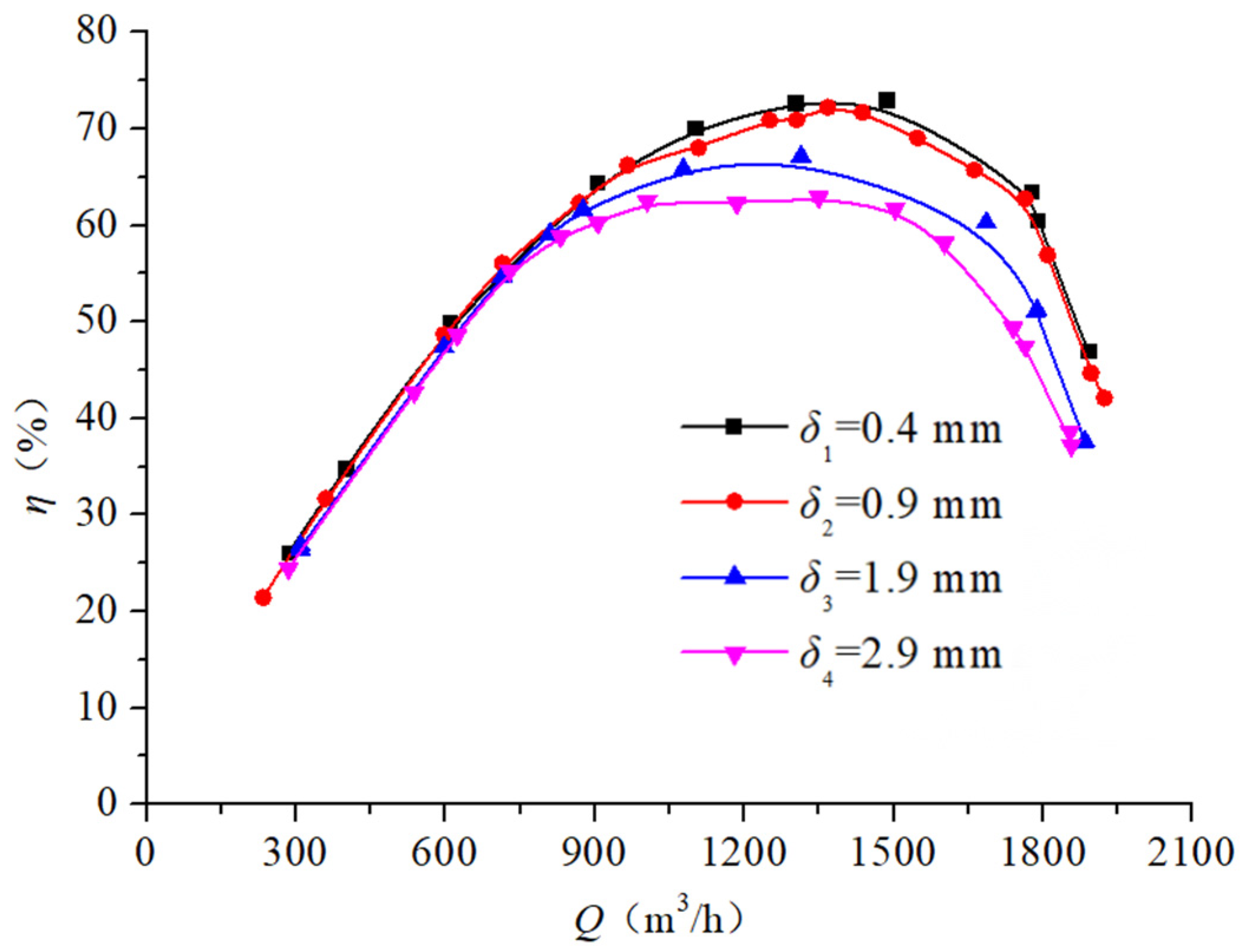
3.2. Experimental Research of the Effect of Different Seal Ring Clearances on the External Characteristics of the Pump

The seal ring is a change in the impeller seal that affects the amount of leakage and significantly impacts the external characteristics of the pump. As shown in Figure 8, the common seal ring structure has a clearance δ. Under normal conditions, prolonged operation leads to wear of the impeller seal ring, resulting in gradual changes in the pump’s external characteristics.

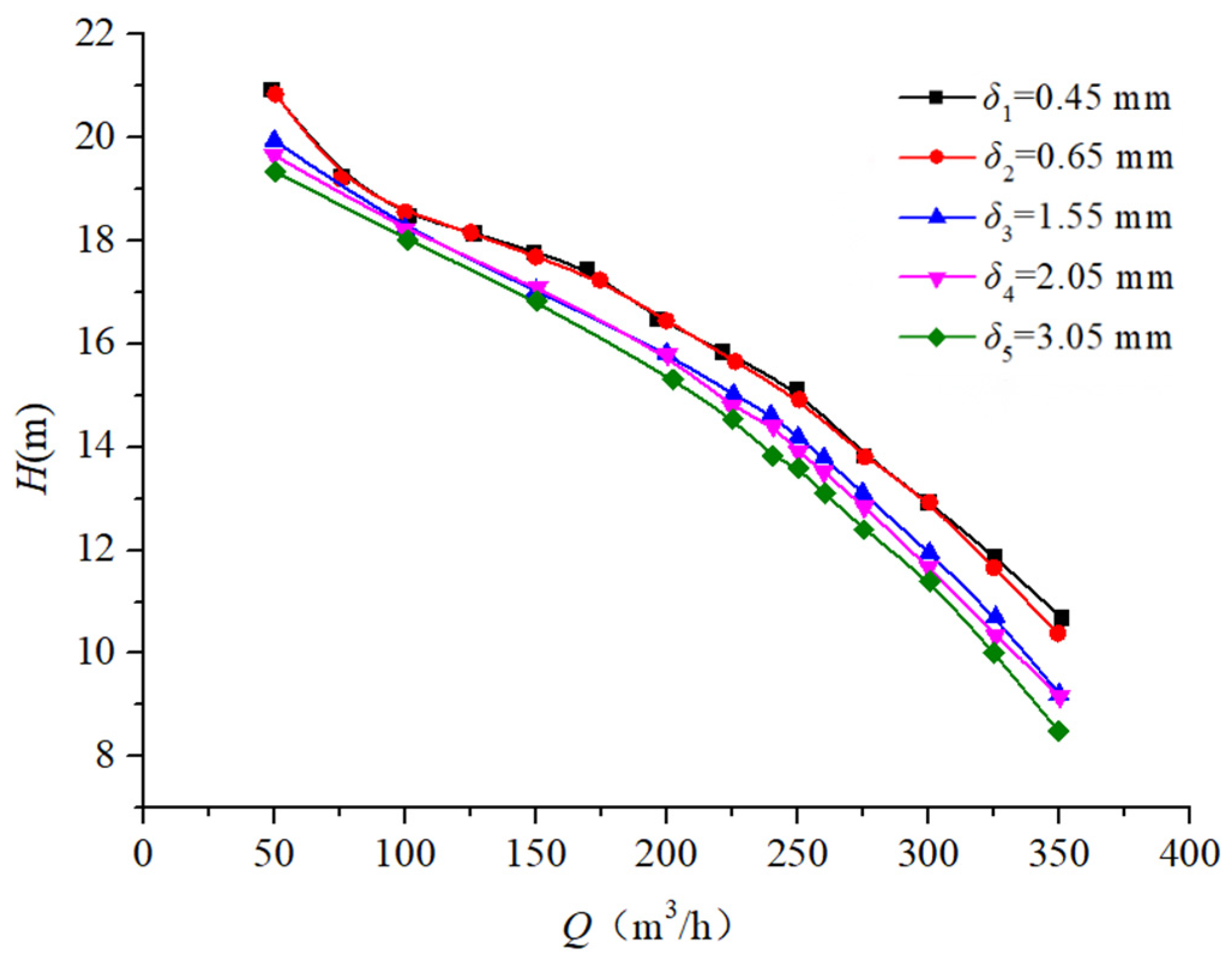
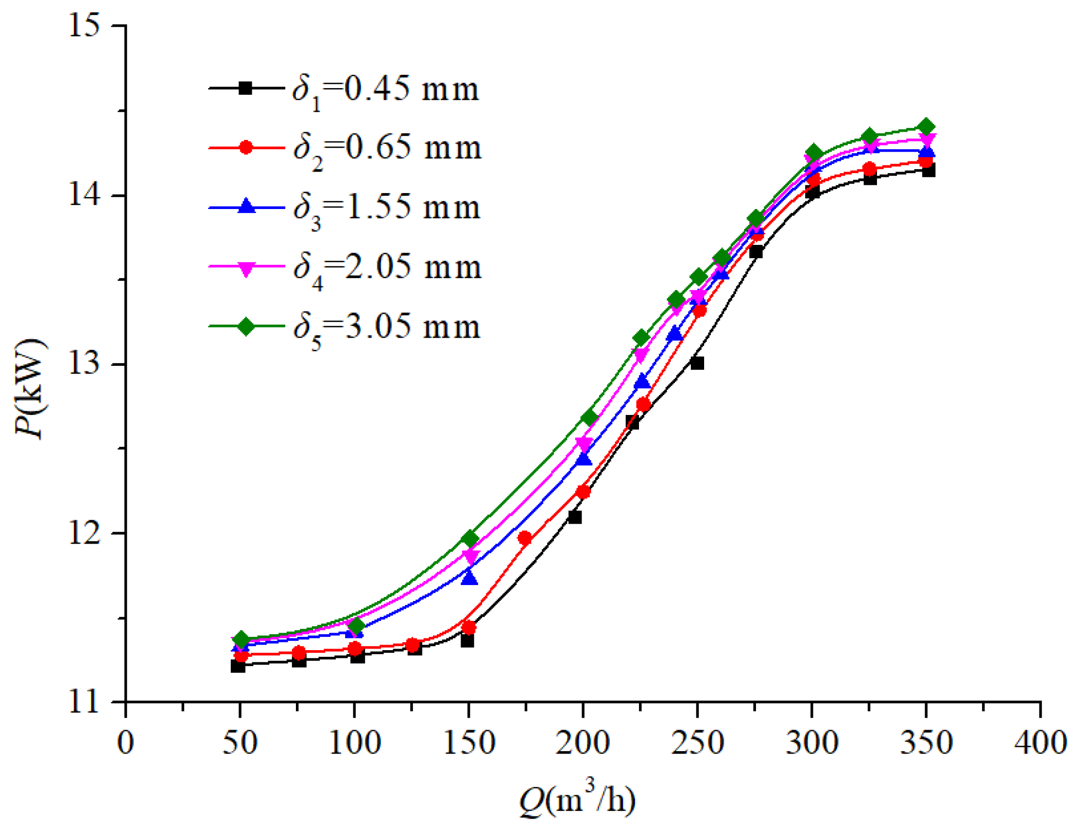
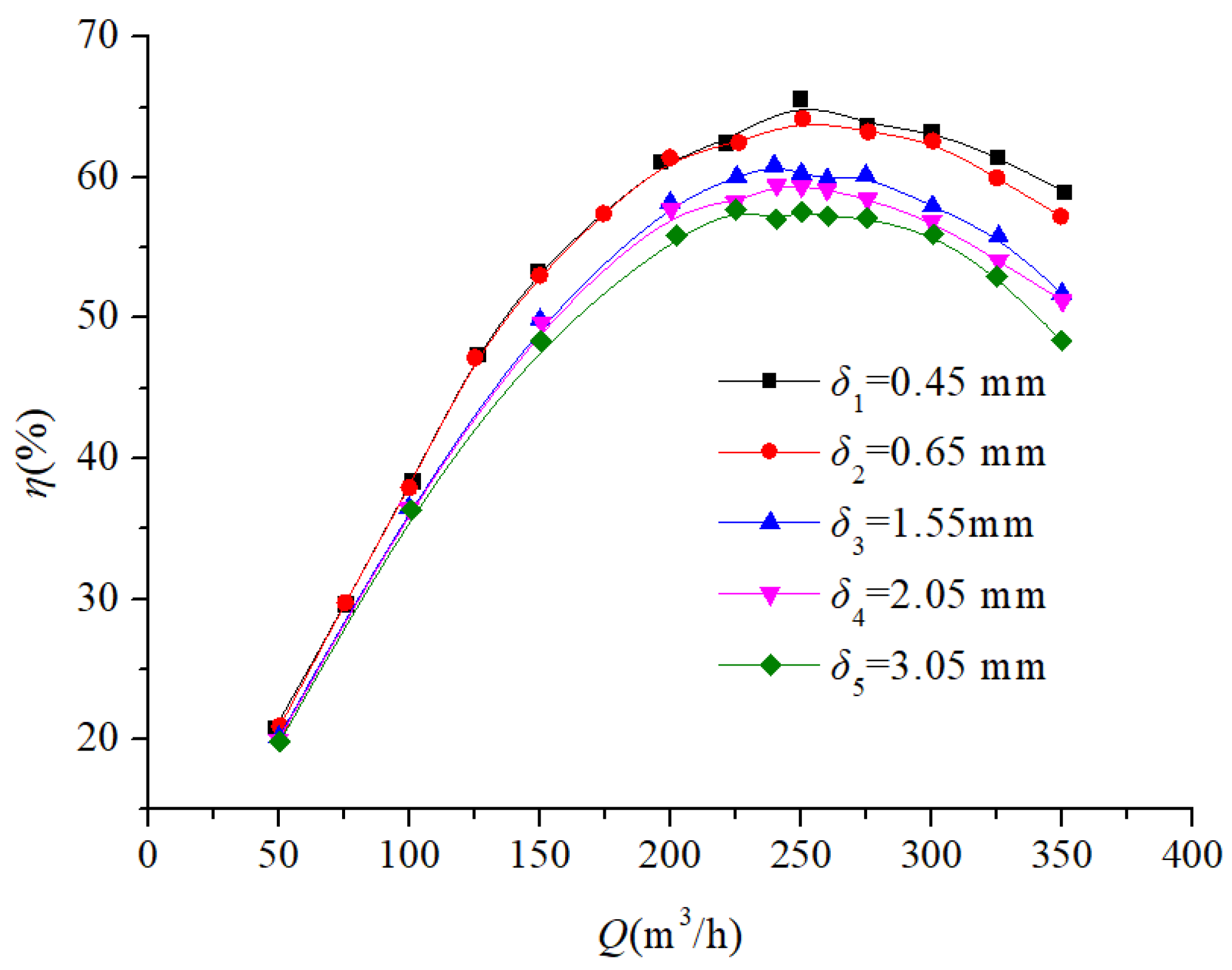
3.2.1. Effect of Different Seal Ring Clearances on Pump External Characteristics at a Speed of ns = 96.2

It can be seen from Figure 9, at a speed of ns = 96.2, that the pump head curve shows distinct behavioral changes when the clearance increases from 0.45 mm to 2.55 mm. When the clearance variation is below 0.2 mm, the head remains virtually unchanged. However, when the clearance change value exceeds 0.6 mm, the head begins to change significantly. With an increase in the clearance value, the head gradually decreases, but the decrease is small. The head is 0.93 m under the 1.2Q condition and 0.24 m under the 0.6Q conditions.
Figure 10 illustrates that the pump power curve changes at ns = 96.2, when the seal ring clearance increases from 0.45 mm to 2.55 mm. When the clearance change is below 0.2 mm, the power remains essentially constant. When the clearance change increases to 0.6 mm, the power begins to change significantly. As the clearance value increases further, the power gradually increases, but the increase is not large. The maximum power increase is 1.18209 kW under the 1.2Q condition, and the lowest power is 0.4629 kW under the 0.6Q conditions.
Figure 11 demonstrates the impact of seal ring clearance variation on the pump efficiency at ns = 96.2 when the clearance increases from 0.45 mm to 2.55 mm. When the clearance change is below 0.2 mm, the power remains essentially constant. When the clearance change increases to 0.6 mm, the efficiency begins to change significantly. As the clearance value increases, the efficiency gradually decreases and reaches 1.6% under the 1.2Q operating conditions.
The curve variation trends observed in Figure 9, Figure 10 and Figure 11 after changing the clearance of the seal ring showed that excessive clearance between the impeller and pump casing creates leakage pathways, allowing working fluid to bypass the impeller. This will lead to a decrease in the flow rate and head of the pump, thus reducing the efficiency of the pump and causing an increase in the shaft power of the pump.

3.2.2. Effect of Different Seal Ring Clearances on Pump External Characteristics at a Speed of ns = 185.5

Figure 12 demonstrates the effect of the seal ring clearance variation on the pump head characteristics at ns = 185.5 as the clearance increases from 0.45 mm to 3.05 mm. When the clearance change is below 0.2 mm, the head has almost no change. When the clearance change increases to 1.1 mm, the head begins to change significantly. With the increase in the clearance, the head gradually decreases, but the decline is not large. The maximum and minimum reductions are 2.21 m under 1.4Q and 0.95 m under 0.6Q operating conditions.
Figure 13 demonstrates the effect of seal ring clearance variation on the pump head characteristics at ns = 185.5 as the clearance increases from 0.45 mm to 3.05 mm. When the clearance change is below 0.2 mm, the power hardly changes. When the clearance change increases to 1.1 mm, the power begins to change significantly. As the clearance value increases, the power gradually increases, but the increase is small; the power rise is 0.60317 kW under 0.6Q and 0.23068 kW under 1.2Q operating conditions.
It can be seen from Figure 14 that the pump efficiency curve changes when the seal ring clearance increases from 0.45 mm to 3.05 mm at ns = 185.5. When the clearance change below 0.2 mm, the efficiency hardly changes. When the clearance change increases to 1.1 mm, the efficiency begins to change significantly. As the clearance increases, the efficiency decreases gradually, with an efficiency drop of at least 4.78% and up to 10.59%. As the clearance of the seal ring increases, the leakage and the flow loss will increase. This will lead to a decrease in the pump’s head and volumetric efficiency, thus causing an increase in the shaft power.

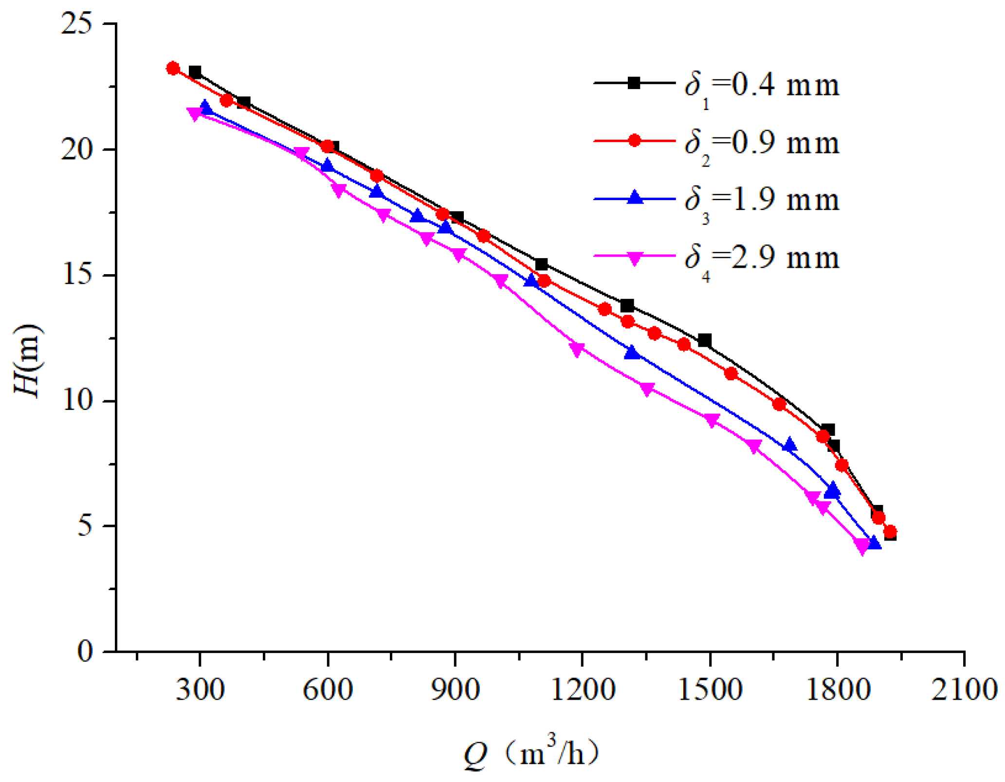
3.2.3. Effect of Different Clearances on Pump External Characteristics at a Speed of ns = 493.3

It can be seen from Figure 15 that the pump head curve changes when the clearance increases from 0.4 mm to 2.9 mm at ns = 493.3. When the clearance change is below 0.5 mm, the head exhibits minimal changes, whereas when the clearance change increases to 1.5 mm, the head begins to change significantly. With the increase in the clearance, the head gradually decreases, but the decline is not large. The maximum drop of the head is 3.07 m under 1.27Q and the minimum is 1.71 m under 0.43Q conditions.
Figure 16 demonstrates the variation in the pump power characteristics with seal ring clearance at ns = 493.3. As the clearance increases from 0.4 mm to 2.9 mm. The shaft power initially decreases, then increases, before decreasing again. This trend contrasts with the power curves observed in low-to-medium specific speed pumps (ns < 300) and is characteristic of mixed-flow impeller designs. The observed trend matches the typical shaft power characteristics of mixed-flow sewage pumps, consistent with established research findings [27]. When the clearance change is below 0.5 mm, the power changes significantly. As the clearance value increases, the power gradually decreases. The maximum power drop is 8.804 kW under 1.27Q and the minimum power is 2.544 kW under 0.43Q conditions.
Figure 17 shows the pump efficiency curve changes when the seal ring clearance increases from 0.4 mm to 2.9 mm at ns = 493.3. When the clearance change is below 0.5 mm, the efficiency shows minimal variation. When the change is beyond 1.5 mm, the efficiency begins to change significantly. As the clearance value increases, further clearance enlargement leads to progressive efficiency degradation, reaching maximum reductions of 16.03% under 1.27Q and 3.66% under 0.43Q operating conditions.

3.3. Intelligent Monitoring System for Pumps Based on Soft Measurement

This study establishes the relationship between the Q-H, Q-P, and Q-η curves and implements a soft measurement approach to determine pump power through auxiliary variable measurement, thereby avoiding the direct measurement of challenging flow parameters.
In this subsection, an intelligent monitoring system based on the soft measurement was designed, combined with cost factors and actual control requirements. The CPU module of PLC 200SMART is used as the control core.

3.3.1. Functional Requirements of the Monitoring System

  • Data acquisition—collect the pump’s operating parameters, including current, voltage, frequency, power, and liquid level. Data processing—calculate derived parameters through processing, including the flow, head, etc. Data storage—temporarily retains processed and raw data for monitoring and analysis.
  • Status display and parameter setting functions, which can collect the parameters, and set the control thresholds (including start/stop levels).
  • Alarm function, which analyzes the collected data in real time; if the liquid level exceeds predefined thresholds, it will cause alarm events with timestamped records.
  • Remote monitoring function, in which all collected data can be displayed visually in real time through a mobile application and industrial cloud platform.
In this paper, test data were collected for a pump with a rated flow of 290 m3/h and a head of 102 m, and the relative error of the flow, head, and efficiency was solved to judge the accuracy of the software system. As shown in Table 5, the system maintains relative errors below 0.5% across most operating conditions (0.1Q–1.3Q), with slightly higher fluctuations (3–4%) observed at extreme operating points. The distribution of other high-density data around the measurement points ensures reliable soft measurement results. An adequate quantity and proper spatial distribution of initial data points are essential to minimize errors. Error occurrence correlates strongly with insufficient valid data points in the vicinity of the target measurement location, highlighting the importance of comprehensive initial data collection.

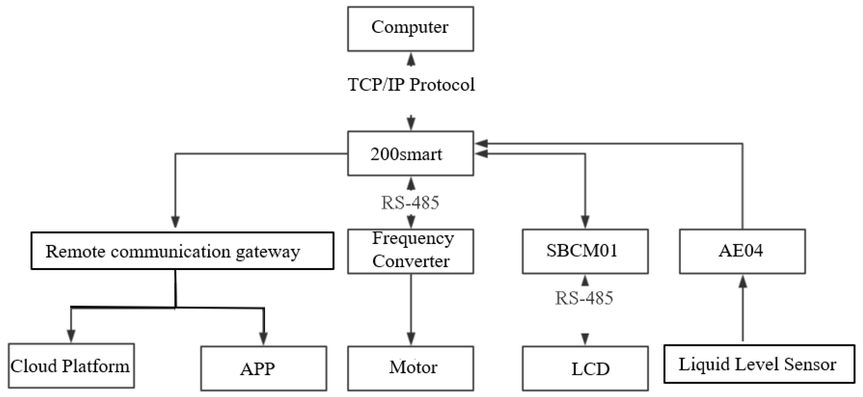
3.3.2. Hardware System in the Monitoring System

The hardware system relationship structure is shown in Figure 18. With the PLC200 smart CPU module as the central processing unit, the expansion module includes an AE04 analog input module and SBCM01 communication expansion board. The SBCM01 module is connected to the inverter and the touchscreen through an RS485 communication line. The PLC obtains the inverter’s current, voltage, frequency, power, and other parameters through the MODbus-RTU communication protocol. The inverter controls the speed through an inverter–motor linkage. The AE04 analog module is connected to the level sensors, while the PLC is connected to the remote communication gateway via the TCP/IP protocol. The remote communication gateway sends data to the mobile application and the cloud platform. The host computer deploys the Step 7 program to the PLC while enabling data feedback to the monitoring terminal. The communication protocol between the computer and the PLC is TCP/IP.
Figure 19 shows the actual diagram of the PLC control cabinet. The numbers in the figure indicate the following elements:
  • The power switch of the control cabinet, which is responsible for the power switch of the whole cabinet.
  • A transformer, which is used to convert the input 240 V voltage into 24 V voltage to supply power to the CPU.
  • A 200smart CPU. When the indicator light is green, it means that the CPU is running normally.
  • The AE04 analog module. When the indicator light is green, the module is running normally.
  • The SBCM01 communication expansion board.
  • The remote communication gateway. When the display light is blue, the gateway communication is normal.
  • An analog input port.
  • The power output interface.
  • The power input interface.
  • The inverter.
  • A liquid crystal display.

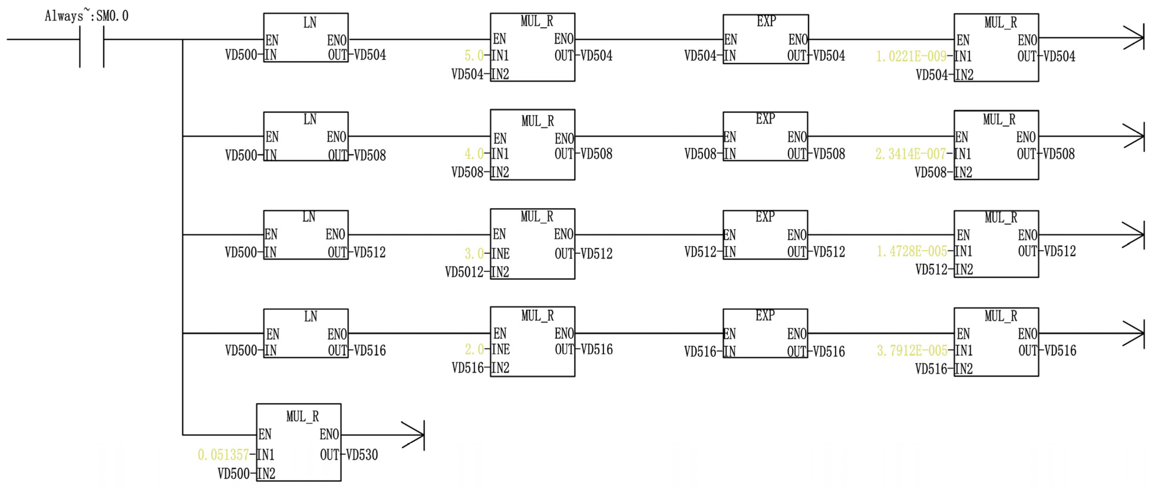
3.3.3. Monitoring System Software

The specific parameters of the pump are as follows: 100 QW-80-6-2.2; the diameter is 100 mm; the rated flow is 80 m3/h; the rated head is 6 m; the rated power is 2.2 kW; the rated speed is 980 r/min; and the number of motor stages is 6.
It is determined that the Q-H curve is a 5th degree polynomial fitting, and the Q-P curve is a second-degree polynomial fitting.
The formula of the Q-H curve is:
H = −1.6775e – 9 × Q5 + 5.5417e – 7 × Q4 − 7.0749e – 5 × Q3 − 0.0041525 × Q2 − 0.13942Q + 9.9271
The formula of the Q-η curve is:
P = 5.5773 × 10 − 5Q2 + 0.0025071Q + 1.2306
The inverse function of the flow–power curve is obtained by Matlab. The procedure is as follows:
syms x;
f = sym (5.5773e – 5 × (x2) + 0.0025071 × x + 1.2306);
finverse (f).
The Q-H and Q-P characteristic curves are programmed into the PLC’s Step 7 environment, with a partial program logic diagram displayed in Figure 20. The PLC obtains variable parameters such as power, current, voltage, and frequency from the inverter and the sensor. The data acquisition Step 7 program is shown in Figure 21. After processing and calculation, the data are transmitted to the computer and the remote communication gateway. Data can be displayed on WINCC via PC Access and further processed and stored in real time. The remote communication gateway sends the data transmitted from the PLC to the mobile phone through the 4G signal, and the data can be displayed on the mobile phone application in real-time.

4. Conclusions

(1)
Compared with the centrifugal pump flow Q-H and Q-P curves with a speed lower than 300, the Q-η curve displays third-order polynomial fitting. The Q-H and Q-P curves of the axial flow pump with a rotational speed higher than 500 are fitted by a piecewise interpolation polynomial; the first segment is a second-order polynomial and the remaining segments are third-order polynomials. However, the Q-η curve retains third-order polynomial fitting. In the mixed-flow pump with speeds between 300 and 500, the Q-H curve adopts the same fitting method as the centrifugal pump. The Q-P curve uses the same fitting method as the axial pump. The Q-η curve is fitted with a third-order polynomial.
(2)
The characteristic curves (Q-H, Q-P, and Q-η) are typically fitted using third- to fourth-order polynomials. The maximum polynomial order without inflection points is 3, the maximum polynomial order of inflection points is 4, and the two inflection points are fitted by segmentation.
(3)
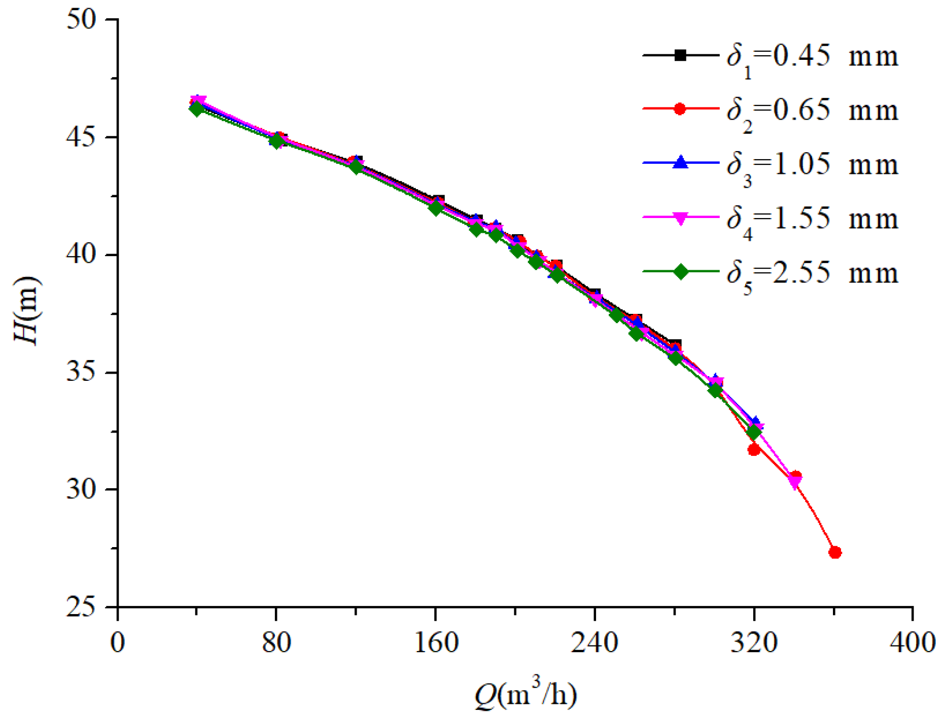
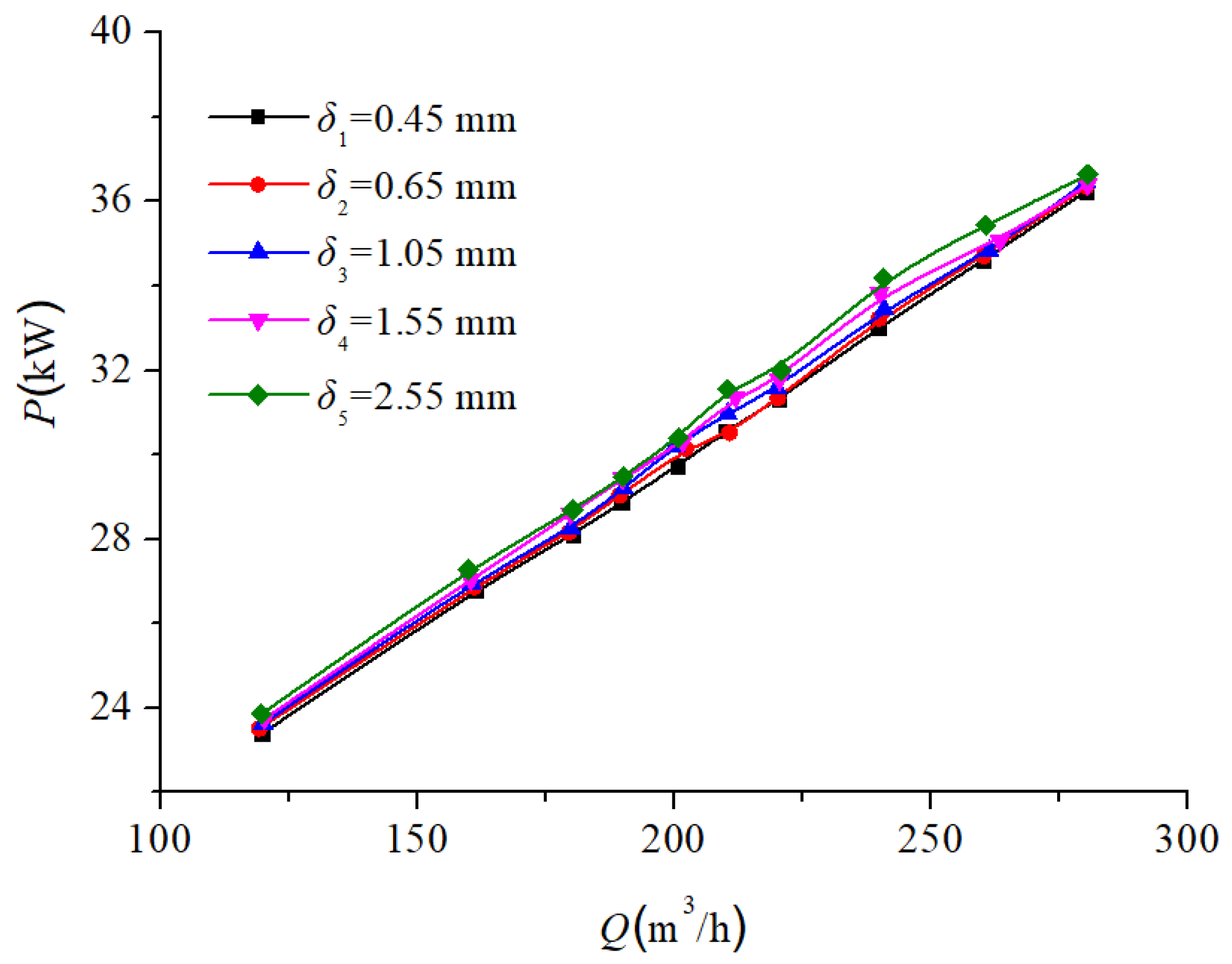
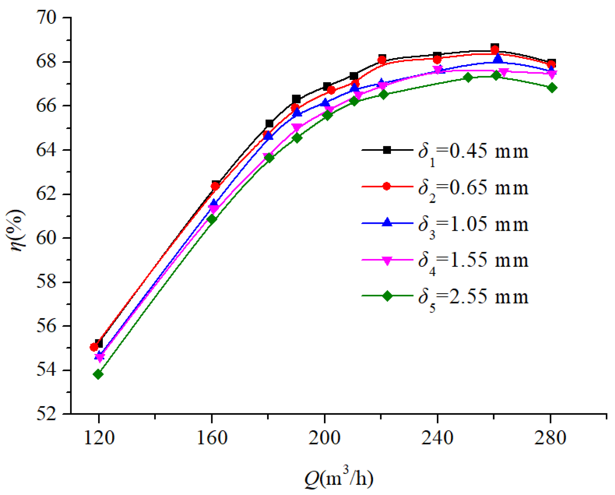
This study investigates pumps with specific speeds of 96.2, 185.5, and 493.3, systematically analyzing the impact of seal ring clearance variations on the pump performance through external characteristic testing. Progressive decreases in both the head and efficiency occur with increasing seal ring clearance, while the shaft power of the pump presents different variation trends with the increase in the specific speed. When the specific speed is low–medium, the shaft power of the pump gradually increases. However, when the specific speed is relatively high (ns > 300), the shaft power initially decreases, then increases, and finally decreases again.
(4)
This paper presents a remote monitoring system and utilizes motor power as the auxiliary variable, using the soft measurement method to ensure that the relative measurement error is <0.5%. All parameters can be displayed via an LCD screen, computer, mobile application, and industrial cloud platform, comprising an integrated alarm system for abnormal conditions. Programmable liquid level thresholds (start/stop) are presented via the LCD interface.

Author Contributions

Conceptualization, Y.L. and P.L.; methodology, Y.L.; software, P.L.; validation, Y.Z., Y.L. and P.L.; formal analysis, W.Q. and R.Z.; investigation, Y.Z.; resources, P.L.; data curation, W.Q.; writing—original draft preparation, W.Q.; writing—review and editing, P.L.; visualization, R.Z.; supervision, Y.L.; project administration, Y.L.; funding acquisition, P.L. All authors have read and agreed to the published version of the manuscript.

Funding

This research was funded by the Science and technology innovation Program of Hunan Province (grant number 2022RC1140), the Natural Science Foundation of Hunan Province (grant number 2023JJ50088), the Hunan Provincial Department of Education Project (grant number 22A0607), and the key R&D program of Hunan Province (grant number 2024AQ2001).

Data Availability Statement

The raw data supporting the conclusions of this article will be made available by the authors, without undue reservation, to any qualified researcher.

Conflicts of Interest

Author Rongsheng Zhu was employed by the company Jiangsu State Spring Pump Manufacturing Co., Ltd. The remaining author declares that the research was conducted in the absence of any commercial or financial relationships that could be construed as a potential conflicts of interest.

References

  1. Olszewski, P. Genetic optimization and experimental verification of complex parallel pumping station with centrifugal pumps. Appl. Energy 2016, 178, 527–539. [Google Scholar] [CrossRef]
  2. Fetyan, K.; El_Gazzar, D. Effect of motor vibration problem on the power quality of water pumping stations. Water Sci. 2014, 28, 31–41. [Google Scholar] [CrossRef]
  3. Mohamed, M.M.A.; Abdellatif, M.M. Flow Improvement at Pump Intake by the Use of Baffle Posts. Beni-Suef Univ. J. Basic Appl. Sci. 2017, 6, 127–137. [Google Scholar] [CrossRef]
  4. Joo, J.G.; Jeong, I.S.; Kang, S.H. Deep Reinforcement Learning for Multi-Objective Real-Time Pump Operation in Rainwater Pumping Stations. Water 2024, 16, 3398. [Google Scholar] [CrossRef]
  5. Moreno-Rodenas, A.M.; Duinmeijer, A.; Clemens, F.H. Deep-learning based monitoring of FOG layer dynamics in wastewater pumping stations. Water Res. 2021, 117482. [Google Scholar] [CrossRef]
  6. Shaazizov, F. Accounting for the energy efficiency of the operation of pumping equipment in the monitoring system of large pumping stations of the Republic of Uzbekistan. E3S Web of Conf. 2023, 410, 8. [Google Scholar] [CrossRef]
  7. Yang, W. Checking the Characteristics of Centrifugal Pump Working Condition by Using Motor Running Current. Equip. Manag. Maint. 1997, 4, 28–29. [Google Scholar]
  8. Guo, L.; Hao, B.; Liu, Y. Research and Application of the Remote Data Monitoring for GSHP(Ground Source Heat Pump) based on MODBUS and TCP/IP Protocol. In Proceedings of the International Conference on Management Science and Intelligent Control(ICMSIC 2011), Hefei, China, 24–26 August 2011; pp. 24–34. [Google Scholar]
  9. Niu, G. Working Condition Detection System Based on Vibration Signal Analysis; Harbin Institute of Technology: Harbin, China, 2016. [Google Scholar]
  10. Song, M.; Wang, T.; Dang, B. Intelligent Calibration of Submersible Electric Pump Monitoring System Based on LabVIEW. Mech. Eng. Autom. 2016, 147–149. Available online: https://xueshu.baidu.com/usercenter/paper/show?paperid=9b1d8c9f0279ca147b59c3fe13c97fec&site=xueshu_se (accessed on 7 May 2025).
  11. Panaras, G.; Mathioulakis, E.; Belessiotis, V. A method for the dynamic testing and evaluation of the performance of combined solar thermal heat pump hot water systems. Appl. Energy 2014, 114, 124–134. [Google Scholar] [CrossRef]
  12. Chen, C. Design and Implementation of Intelligent Monitoring System for Sewage Pumping Station. Archit. Eng. Technol. Des. 2018, 12, 959. [Google Scholar]
  13. Bian, Y.; Yang, Y.; Guo, Z. Design of Computer Monitoring System for Pumping Stations in Water Conservancy Irrigation District. J. Autom. 2018, 39, 94–96. [Google Scholar]
  14. Schleer, M.; Abhari, R.S. Clearance Effects on the Evolution of the Flow in the Vaneless Diffuser of a Centrifugal Compressor at Part Load Condition. J. Turbo Mach. 2008, 130, 79–87. [Google Scholar] [CrossRef]
  15. Langthjem, M.A.; Olhoff, N. A numerical study of flow-induced noise in a two-dimensional centrifugal pump. Part I. Hydrodynamics. J. Fluids Struct. 2004, 19, 349–368. [Google Scholar] [CrossRef]
  16. Dular, M.; Bachert, R.; Stoffel, B.; Širok, B. Experimental evaluation of numerical simulation of cavitating flow around hydrofoil. Eur. J. Mech.-B Fluids 2005, 24, 522–538. [Google Scholar] [CrossRef]
  17. Choi, C.-H.; Noh, J.-G.; Kim, D.-J.; Hong, S.S.; Kim, J. Effects of floating-ring seal clearance on the pump performance for turbopumps. J. Propuls. Power 2009, 25, 191–195. [Google Scholar] [CrossRef]
  18. Lomakin, A. Calculation of critical speed and securing of dynamic stability of hydraulic high-pressure pumps with reference to the forces arising in the gap seals. Energomashinostroenie 1958, 4, 1158. [Google Scholar]
  19. Ayad, A.F.; Abdalla, H.M.; Aly, E.A. Effect of semi-open impeller side clearance on the centrifugal pump performance using CFD. Aerosp. Sci. Technol. 2015, 47, 247–255. [Google Scholar] [CrossRef]
  20. Zhou, Z.; Wang, H.; Wang, Y.; Li, X.; Lin, Q. Influence of ring clearance on the performance of two-stage high-speed centrifugal pumps. J. Rocket Propuls. 2023, 49, 66–72. [Google Scholar]
  21. Zhao, C.; Han, X.; Cui, Z. Numerical simulations of flow characteristics of wear-ring clearance in the centrifugal pump. Chin. J. Ship Res. 2020, 15, 159–167. [Google Scholar]
  22. Gao, B.; Wang, Z.; Yang, L.; Du, W.; Li, C. Effect of wear-ring clearance on performance and flow characteristics of centrifugal pump. J. Drain. Irrig. Mach. Eng. (JDIME) 2017, 35, 13–17. [Google Scholar]
  23. Zhao, W.; Wu, G.; Li, Y.; Wang, Y. Study on effects of wear-rings clearance modifications on performance of centrifugal pump. J. Hydroelectr. Eng. 2014, 33, 211–215. [Google Scholar]
  24. Chen, Y.; Fei, Z.; Cai, Y.; Yang, R.; Li, W. Effect of the clearance of wear-rings on the performance of centrifugal oil pump while handling water. Fluid Mach. 2006, 34, 1–5. [Google Scholar]
  25. Fu, Q.; Chen, Y.; Huang, Q.; Zhu, R.; Wang, X. Influence of front ring clearance on internal flow characteristics of centrifugal pump. J. Chongqing Univ. Technol. Nat. Sci. 2022, 36, 203–209. [Google Scholar]
  26. ISO 9906; Rotodynamic Pump-Hydraulic Performance Acceptance Tests-Grades 1 and 2. International Standardization Orgnization: Geneva, Switzerland, 1999.
  27. Guan, X. The Hydraulic Design of Centrifugal Pumps and Mixed-Flow Pumps. In Modern Pumps Theory and Design; China Astronautic Publishing House: Beijing, China, 2011; pp. 241–265. [Google Scholar]
  28. Wu, X.; Ding, D.; Hu, S. Fitting and Mapping of Characteristic Curve of Centrifugal Pump Based on MATLAB. China Rural. Water Hydropower 2010, 144–146. Available online: https://irrigate.whu.edu.cn/EN/Y2010/V0/I11/144 (accessed on 7 May 2025).
  29. Liu, H.; Sun, T.; Liu, W.; Wang, L.; Wei, J. Fitting of Centrifugal Pump Performance Curve Based on Visual Basic Programming. Contemp. Chem. Ind. 2014, 43, 648–651. [Google Scholar]
  30. Du, D.; Liu, Q.; Fang, G.; Wang, Y. Performance Curve Fitting of Pump Based on Polynomial-Markov. J. Hydroelectr. Eng. 2014, 7, 144–146. [Google Scholar]
  31. Tang, Y.; Xiao, M.; Tang, L. Piecewise least squares polynomial fitting algorithm for pump performance curve. J. Drain. Irrig. Mach. Eng.(JDIME) 2017, 35, 744–748. [Google Scholar]
  32. Dharmarajan, R.; Rowley, P.; Stein, J.; Scott, S. Performance Validation and Curve Fit Generation of Natural Gas and Electric Heat Pump VRF Systems. ASHRAE Trans. 2024, 130, 466–474. [Google Scholar]
Figure 1. Three kinds of submersible pumps with different specific speeds. (The calculation formula is shown in Formula (3)).
Processes 13 01529 g001
Figure 2. System structure diagram of the experimental pipeline of the submersible pumps.
Processes 13 01529 g002
Figure 3. Specific speed calculation and data import interface.
Processes 13 01529 g003
Figure 4. Test error data correction interface.
Processes 13 01529 g004
Figure 5. Comparison of Q-H curve 2–6 polynomial fitting.
Processes 13 01529 g005
Figure 6. Comparison of Q-P curve 2–6 polynomial fitting.
Processes 13 01529 g006
Figure 7. Centrifugal pump performance curve fitting diagram.
Processes 13 01529 g007
Figure 8. Seal ring structure of the pump.
Processes 13 01529 g008
Figure 9. Changes in the head of different clearance schemes.
Processes 13 01529 g009
Figure 10. Power variation under different clearance schemes for a 96.2 pump.
Processes 13 01529 g010
Figure 11. Change in efficiency for different clearance schemes at a speed of 96.2.
Processes 13 01529 g011
Figure 12. Comparison of different seal ring clearance heads at a speed of 185.5.
Processes 13 01529 g012
Figure 13. Comparison of the power of five different clearance schemes for centrifugal pumps at a speed of 185.5.
Processes 13 01529 g013
Figure 14. Comparison of the efficiency of five different clearance schemes at a specific speed of 185.5.
Processes 13 01529 g014
Figure 15. Comparison of the head of four different seal ring clearances at a specific speed of 493.3.
Processes 13 01529 g015
Figure 16. Comparison of the power of the four different seal ring clearances with a specific speed of 493.3.
Processes 13 01529 g016
Figure 17. Comparison of the efficiency of the four different seal ring clearances with a specific speed of 493.3.
Processes 13 01529 g017
Figure 18. Hardware relationship structure diagram.
Processes 13 01529 g018
Figure 19. Actual diagram of the PLC control cabinet.
Processes 13 01529 g019
Figure 20. Calculation program in PLC.
Processes 13 01529 g020
Figure 21. Step 7 program.
Processes 13 01529 g021
Table 1. Specific parameters of three kinds of submersible pumps.
Pump Parameters150 QW-260-38-45200 QW-250-15-15350 QW-1388-13-90
Rotational speed (r/min)148014801480
Flow rate (m3/h)2602501388
Head (m)37.281512.88
Power (kW)451590
Specific speed96.2185.5493.3
Pipe diameter (mm)150150350
Table 2. Centrifugal pump external characteristic data.
Flow m3/hHead mPower kWEfficiency %
0137.5661.119310
104124.4268.5359551.43
152120.4677.6238762.45
202115.9388.3960872.17
250109.1596.7827876.8
268106.16100.0530677.46
294101.85104.1513678.32
298100.69104.6578.1
31298.16106.3547678.45
34889.82110.391177.14
37283.92111.8977676
43464.35112.2335667.79
Table 3. Comparison of Q-H and Q-P curve fitting error parameters of 2nd~6th order fitting times.
2nd Order3rd Order4th Order5th Order6th Order
Correlation coefficientQ-H0.994830.999760.999930.999970.99997
Q-P0.980610.999570.999910.999960.99996
Root mean squareQ-H1.90190.409610.222010.141790.13811
Q-P3.2730.490890.222980.156860.15685
Absolute error maximumQ-H3.71960.854920.482820.234890.23047
Q-P6.01451.05070.579960.347960.34713
Relative error maximumQ-H1.5177%0.296%0.1544%0.11364%0.10696%
Q-P2.6647%0.3645%0.16915%0.11867%0.l1802%
Table 4. Axial flow pump external characteristic data.
Flow m3/hHead mPower kWEfficiency %
420.399.6232.1718434.25
479.238.8830.2232738.37
498.888.1428.3062139.1
524.647.6927.1052840.52
586.268.0329.4425343.54
646.638.2428.9955850.06
696.558.1528.7960753.72
748.227.9228.6684456.28
780.487.3927.6921156.71
862.067.1527.4717861.08
910.22726.913864.45
999.186.3425.5867367.47
Table 5. Relative error table for solving flow, head, and efficiency.
Actual Power (kW)Solving Flow (m3/h)Solving Head (m)Solving
Efficiency
Actual Flow (m3/h)
61.1193139.2048131.504522.963%0
68.53595103.2173124.726951.135%104
77.62387151.9494120.415264.167%152
88.39608204.5221115.135372.517%202
96.78278248.0516109.501676.399%250
100.05306267.0092106.558577.412%268
104.15136293.9204101.791978.199%294
104.650297.5546101.092378.247%298
106.35476310.855198.41478.304%312
110.3911352.643188.759377.186%348
111.89776380.503581.258575.219%372.01
Actual Head (m)Actual EfficiencyRelative Error of FlowRelative Error of HeadRelative Error of Efficiency
137.560−inf−4.402%inf
124.4251.43%0.75263%0.24605%−0.57376%
120.4664.25%0.033315%−0.03716%−0.12991%
115.9372.17%−1.2486%−0.68554%0.48067%
109.1576.8%0.77937%0.32214%−0.52206%
106.1677.46%0.36969%0.37538%−0.06212%
101.8578.32%0.027088%−0.05705%−0.15443%
100.6978.1%0.14947%0.3995%0.18849%
98.1678.45%0.36696%0.25876%−0.18667%
89.8277.14%−1.3342%−1.11809%0.05966%
83.9276%−2.2831%−3.1715%−1.0272%
Disclaimer/Publisher’s Note: The statements, opinions and data contained in all publications are solely those of the individual author(s) and contributor(s) and not of MDPI and/or the editor(s). MDPI and/or the editor(s) disclaim responsibility for any injury to people or property resulting from any ideas, methods, instructions or products referred to in the content.

