Long Short-Term Memory Networks for State of Charge and Average Temperature State Estimation of SPMeT Lithium–Ion Battery Model

Abstract

Lithium–ion batteries are the dominant battery type for emerging technologies in the efforts to slow climate change. Accurate and quick estimations of state of charge (SOC) and internal cell temperature are vital to battery-management systems to enable the effective operation of portable electronics and electric vehicles. Therefore, a long short-term memory (LSTM) recurrent-neural network is proposed which completes the state estimation of SOC and internal average cell temperature (Tavg) of lithium–ion batteries under varying current loads. The network is trained and evaluated using data compiled from a newly developed extended single-particle model coupled with a thermal dynamic model. Results are promising, with root mean square values typically under 2% for SOC and 1.2 K for Tavg, while maintaining quick training and testing times. In addition, we examined a comparison of a single-feature versus multi-feature network, as well as two different approaches to data partitioning.

1. Introduction

As a result of the ongoing climate crisis, alternatives to traditional forms of energy such as coal and gas are becoming more and more popular [1,2,3]. Lithium–ion batteries are a promising candidate for energy-storage systems, and are already being used in many portable applications and electric vehicles [1,2,3,4,5]. A battery-management system (BMS) is what controls the battery during operation, and relies on accurate data to operate effectively [2,5,6]. One key parameter to BMS operations is state of charge (SOC); SOC quantifies the difference between a battery in use and its nominal/fully charged capacity [2,5,6,7,8,9]. Another very important characteristic when it comes to battery control and design is the internal temperature of the cell [3,10,11]. Several safety concerns arise when operating batteries if the internal temperature is outside the appropriate limit, in addition to accelerated degradation and poor performance [3,10,11]. Therefore, it is vital to have an accurate estimation of the internal temperature of a cell during charging/discharging under varying current loads. Moreover, the speed of obtaining these estimations (SOC and temperature) must be fast enough to be utilized in real-time applications [2,3,5,6,7,8,9,10,11].

The estimation of SOC has been extensively studied, and may be separated into four main categories: direct measurement methods, book-keeping methods, adaptive methods, and hybrid methods [9]. Given the recent advancements in machine learning (ML) and studies of deep learning networks, there is increasing interest in utilizing data-driven and algorithm approaches instead of more traditional methods. The general idea behind machine learning is that an algorithm is utilized to learn a pattern between a set of inputs and outputs [12]. There are two primary categories of machine learning: statistic-based learning, and neural networks. While statistic-based learning has its merits, the more suitable approach in this case is the use of neural networks; neural networks typically show better RMSE values than that of conventional regression methods, and thus are the preferred method of choice for battery state estimation [13]. Some forms of neural networks include convolutional NNs (CNNs) and recurrent NNs (RNNs). While CNNs are efficient at extracting positional invariant features, they are also hierarchical in nature [12,13]. Meanwhile, RNNs provide more flexibility, and are better suited for sequential modelling as they take into account previous state information [12]. The hidden state which is calculated via Equation (1) is what enables this [12].

$$h_t=f_w(h_{t-1},x_t)$$

(1)

where $h_t$ is the new hidden state, $h_{t-1}$ is the old hidden state, $x_t$ is the input vector at some discrete time step t, $f_w$ is a function with parameters w, and w refers to a set of weights [12]. In “vanilla” RNNs’ $f_w$ is often a hyperbolic tangent function to provide nonlinearity [12].

However, traditional RNNs struggle with the so-called vanishing gradients problem [2,12,14]. To handle this issue, the long-short-term-memory (LSTM) network architecture was developed [2,12,14]. LSTM networks are a form of multi-layer RNN, which are composed of four different gates, and have two hidden states (hidden state and cell state) which must be maintained instead of one [2,12,14]. As there are four interacting internal states as opposed to one, LSTM networks can add or remove information to the cell state which preserves the older cell memory after multiple time steps [2,12,14]. Figure 1 outlines the main steps involved in RNNs in general, while Figure 2 illustrates the internal structure of an LSTM network. While studies such as Yi et al. and Jiang et al. have completed SOC estimation for varying ambient temperatures using LSTM, typically the data are obtained from a database or using an equivalent circuit model, which eliminates the reflection of the internal characteristics of the cell during charging [1,3,15]. Most existing approaches are limited in their ability to explicitly capture internal temperature dynamics, primarily due to challenges related to limited observability and nonlinear system behavior. Enhanced estimation of state-of-charge and internal temperature can substantially improve battery performance and safety, with potential benefits such as extended driving range and reduced thermal degradation in electric vehicles [16].

Motivated by the above work and findings, the contribution of this work is to combine “model” and “data-driven” estimation methods using data from previous work [17], considering model-based state estimation of distributed parameter systems is challenging [18]. More specifically, this manuscript generates high-fidelity simulation data using the newly developed extended single-particle model coupled with a thermal model [17], and further leverages the supervised machine learning method, namely, the LSTM algorithm, for estimating both state of charge and average cell temperature for a lithium–ion battery for four different C-Rates. Thus, the generalizability of the previous modelling work is extended, and the internal characteristics of the cell dynamics have some reflection in the estimation of the cell states [9,19].

The contributions of this manuscript are as follows: (1) a new extended single-particle battery PDE model coupled with thermal dynamics is developed and used for high-fidelity simulations and data generation under varying current loads; (2) an LSTM network is proposed for accurate estimation of the state of charge and internal cell temperature in lithium–ion batteries; and (3) the proposed method achieves promising results, with root mean square errors typically under 2% for the state of charge and 1.2 K for the average temperature.

The remainder of this paper is organized as follows: problem formulation which contains a comprehensive literature review and network architecture, discussion, results, and finally conclusions. Additional information such as abbreviations, nomenclature, and hyperparameter definitions can be found in Appendix A, Appendix B and Appendix C, respectively.

2. Problem Formulation

To approach this daunting task, first, a literature review considering state estimation of SOC and internal cell temperature is completed, and the network theory and architecture are reviewed.

2.1. Literature Review

Data-driven methods, such as neural networks, support-vector machines, regression techniques, and more, have been utilized to predict various measures of battery life; namely, the SOC, state of health, and remaining-useful life. Roman et al. designed a machine learning pipeline to estimate battery capacity fade, and then evaluated the model on 179 cells which were cycled under different operating conditions [20]. The process involved refining and substantial testing of ML algorithms for application to capacity fade estimation [20]. Meanwhile, the work of Danko et al. reviewed commonly used SOC estimation methods of all types, with advantages and disadvantages for each method described [21]. Neural networks in this instance/context are classified as an adaptive method; they use mathematical algorithms to process data and solve relations between numerous initial complex components [21].

More specifically, Zhao et al. contribute an extensive review of the three primary steps for completing different types of SOC estimation methods via ML [9]. The advantages and disadvantages of traditional NNs versus deep learning networks are also described [9]. Particularly of note is that traditional methods of SOC determination have difficulty resolving the complex battery models’ responsiveness to model parameters, poor flexibility, and high computational complexity [9]. Such lacking efficiencies which are a consequence of the uncertainty and complexity inherent to most battery models highlight the necessity for further work in real-time capabilities, accuracy, robustness, and flexibility of SOC estimations [9]. One path to improving the accuracy of SOC estimation, generalizability of the models, and overall model performance is the use of high-quality datasets [9]. Such datasets contribute greatly to this field of research by expanding the variability of data, and facilitating more precise predictions and optimizations concerning SOC determination models [9]. Moreover, the comparison of hyperparameters—which are manually manipulated and directly affect model performance and generalizability—is of great interest when reviewing studies pertaining to this topic [9].

Table 1. Hyperparameters for SOC estimation.

Hyperparameters (SOC Estimation)
Parameter	This Paper	Paper [9]	Paper [2]	Paper [5]	Paper [6]
Epochs	150	3000		150	2000
Initial Learning Rate	0.01	0.01	0.01	0.01	0.01
Learning Rate Drop Period	25
Minibatches	32	89	60	64	60
Loss Function Optimizer	ADAM	ADAM	ADAM	ADAM

and

Table 2. Hyperparameters for temperature estimation.

Hyperparameters (Temperature Estimation)
Parameter	This Paper	Paper [9]	Paper [2]	Paper [5]	Paper [6]
Epochs	300	8	1000	5000
Initial Learning Rate	0.01	5		0.01	0.00001
Learning Rate Drop Factor	0.5	0.9999	0.2	0.1	0.1
Learning Rate Drop Period	25		200	1000
Minibatches	32		256
Loss Function Optimizer	ADAM		ADAM		ADAM

compare some of the hyperparameters used in this work with others in the literature, including epochs, initial learning rate, learning rate drop period, minibatches, and loss function optimizer.

Possible evaluation metrics for these models include mean average error (MAE), mean squared error (MSE), and the root mean square error (RMSE) [9]. Typically, most of the studies in the literature use RMSE, and some combination of MSE, MAE, or another form of error value [2,9,21]. Equations (2)–(5) were used to calculate the general standard deviation and standardization, RMSE, and MSE respectively.

$$\sigma =\sqrt{{\displaystyle \frac{1}{n}}\sum _{i=1}^n{(X_i-\mu )}^2}$$

(2)

$$X_{std}={\displaystyle \frac{(X-\mu )}{\sigma }}$$

(3)

$$RMSE=\sqrt{{\displaystyle \frac{1}{n}}\sum _{i=1}^n{(Y_{pred,i}-Y_i)}^2}$$

(4)

$$MSE={\displaystyle \frac{1}{n}}\sum _{i=1}^n{(Y_{pred,i}-Y_i)}^2$$

(5)

where $X_i$ is a general variable X at instance i, $\mu$ is the mean of variable X, n is the size of the population, and $\sigma$ is the standard deviation of X. In this instance, $Y_{pred}$ is the predicted value from the network and $Y_i$ is the testing value from that particular time step. Some of these performance-evaluation metrics will be employed to assess the proposed method in Section 3.

As mentioned in the introduction, the use of LSTM algorithms in this application has been shown to be effective and accurate, with benefits over traditional NNs and some other RNN configurations [9,12,13]. Yang et al. extended a previous study which completed SOC estimation using a gated RNN by proposing an LSTM network to describe the complex behaviors of lithium–ion batteries under diverse ambient temperatures [2,6]. Furthermore, an unscented Kalman filter (UKF) is integrated to filter out noise from the data and provide an even more accurate estimation [2]. The method presented is model-free and entirely data-driven, and provides satisfying SOC estimation under multiple operating temperatures [2]. One particular reason LSTM is more suited for state estimation as opposed to classic RNN configurations is that instead of gradient backpropagation occurring exponentially, the LSTM allows gradient flow to be unchanged by using a cell state [2,12]. Moreover, the four different gates as shown in Figure 2 decide which data are retained vs. “forgotten” and thus able to address long-term dependencies [2,12]. Two major roadblocks with regards to SOC determination from complex battery systems are the inability to cope directly with varying ambient temperatures, and the flat regions of the OCV-SOC curves (especially present in LFP batteries and studies of porous electrode theory) can cause large fluctuations in the SOC due to small errors in voltage measurement [2]. The benefit of using ML methods, and LSTM networks in particular is that these deficiencies may be addressed without increasing the run time of the simulations [2,5]. There must be a trade-off, however, between testing accuracy and training cost; the work of Yang determined an epoch number of approximately 8000, with a 1.7 h training time [2].

There have also been efforts, although more limited than that of SOC estimation, concerning the state estimation of cell temperatures via ML. While traditional methods have been used for temperature estimation such as the measurement-based one as by Richardson et al. or a simplified thermal model combined with a Kalman filter, a common drawback of these approaches is the assumptions required to implement such models [8,15,22]. These assumptions can limit the applicability and reduce the estimation accuracy of the models [15]. Consequently, there have been increased investigations into the use of NNs for the determination of temperature [11,15]. Two types of RNNs, an LSTM and a gated recurrent unit (GRU) algorithm, are proposed for the estimation of the surface temperature of LIBs during discharging under varying ambient temperatures by Jiang et al. [15]. Datasets from the Prognostics Center of Excellence were used to train, validate, and test the two different networks [15]. While in previous studies the temperature was fixed as the output, Jiang et al. elected instead to adopt the temperature difference along the time axis as the output [15]. The results are promising, with both RNN types demonstrating accurate real-time temperature estimation [15]. Additionally, the LSTM network shows better performance in trend tracking of the temperature variance when compared to the GRU NN, although a slightly longer training time is required [15]. Similarly, Cho et al. proposed a hybrid LSTM-physics-informed neural network (PINN) method for estimating LIB pack temperature [10]. In this instance, the algorithm makes use of an exponential function and shows more accurate results for a direct current fast charge protocol [10]. The PINN is an NN-type approach that conducts learning by incorporating physics laws into the loss function; while this method has recently attracted attention in many applications, it does not include representation of the electrochemical mechanics present during discharging/charging of LIBs [10]. Another example of the use of LSTM for temperature prediction is that of Yi et al. [3]. The work demonstrates a digital twin (DT) technology and LSTM-based method for real-time temperature prediction and degradation analysis of lithium–ion batteries [3]. Other techniques aside from LSTM have been utilized in recent studies to capture significant battery dynamics. For example, a data-driven approach to capture degradation dynamics using operable sparse identification of systems (OASIS) was developed by Bhadriraju et al. [23]. The method uses two models (inter- and intra-OASIS) to accurately predict the SOC and voltage dynamics [23]. Another method to predict intra-cycle capacity fade is proposed in the work of Hwang et al, a battery model that combines a form of enhanced SPM model with first principle-degradation mechanics [24]. The newly developed battery model yields a superior current-input profile in terms of intra-cycle capacity fade minimization when compared with the traditional CC-CV charging protocol [24]. Meanwhile, Lee et al. proposed a multi-scale model via a kinetic Monte Carlo approach (kMC) which again acts to capture degradation dynamics (in this case, specifically in the form of dendrite growth in the anode) [25]. The kMC is combined with an SPM-type electrochemical model; thus, the integrated electrochemical model illustrates the macroscopic properties and the kMC model describes the microscopic dynamics [25]. This approach is intriguing as it demonstrates the effect of major variables such as cell voltage and Li–ion concentration on the evolution of microscopic properties [25]. Alternatively, Sitapure and Kwon highlight the potential of transformers by developing, testing, and comparing first-generation time-series transformers (TSTs) with existing models [26]. Additionally, a groundbreaking TST-based model predictive controller (MPC) further demonstrates the impressive capabilities of TSTs [26]. The TSTs possess a parallelization-friendly architecture (in RNN-type sequential models) which allows for the training of extraordinarily large models [26]. This could be applied in implementing more comprehensive battery models to maintain computation speed. The DT model is formulated based on lumped thermal equivalent circuit models (ECMs) to describe the dynamic thermal behavior of LIB cells, and the results from two different C-Rates are compared [3]. This proposed approach provides acceptable accuracy for real-time temperature prediction for the charging process and uses the Pearson correlation coefficient (PCC) to extract parameters displaying high correlation with the DT model parameters from the charging curve [3]. However, ECMs lack representation of the electrochemical dynamics within the cell and thus do not fully describe the internal physical characteristics that occur during charging/discharging cycles [1,3]. Deep learning approaches were combined with Kalman filters to suppress transient signal oscillations and enhance the accuracy of state-of-charge (SOC) estimation in [27,28], which may face drawbacks such as high computational cost and challenges in real-time implementation. A summary of reviewed methods of lithium–ion battery estimation is shown in

Table 3. Summary of reviewed methods for SOC and temperature estimation in lithium–ion batteries.

Methods	Applications	Advantages	Disadvantages
LSTM [6,9,12,13]	SOC estimation	Accurate, model-free	Sufficient data, high compute cost
LSTM + UKF [2]	SOC estimation	Noise filtering, better dynamic performance	High complexity and compute cost
GRU/LSTM [15]	Temperature estimation	Accurate tracking	Sufficient data, high compute cost
LSTM+PINN [10]	Temperature estimation	Incorporates physics, better accuracy	No electrochem. included, complex to train
Digital Twin + LSTM [3]	Temperature prediction, degradation analysis	Real-time prediction	High compute cost
OASIS [23]	SOC and voltage prediction	Interpretable, captures degradation	Model integration complexity
Enhanced SPM + degradation [24]	Intra-cycle capacity fade prediction	Physically grounded, better control input	Electrochem. knowledge needed
kMC + SPM [25]	Demonstrates the effect of major variables	Links micro–macro behavior, interpretable	High computation, complex modelling
Transformers [26]	Battery modelling and MPC	Parallelizable training	Needs large data
DL + Kalman Filter [27,28]	SOC estimation	Suppresses transient oscillations, improves accuracy	High compute cost, real-time implementation limits

, including applications, advantages, and disadvantages. The next section of this paper will discuss LSTM theory in more detail and why it is the chosen algorithm for this problem, as well as the architecture and settings of the developed network.

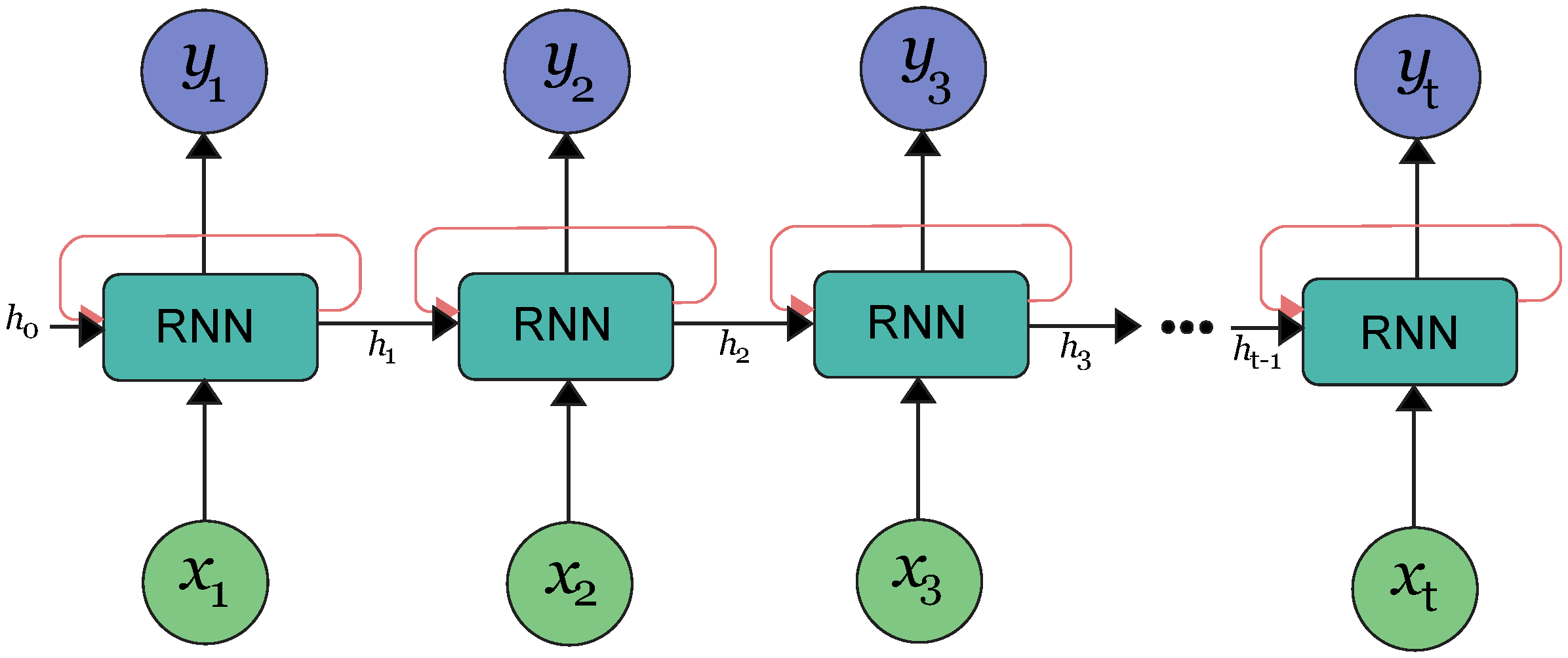
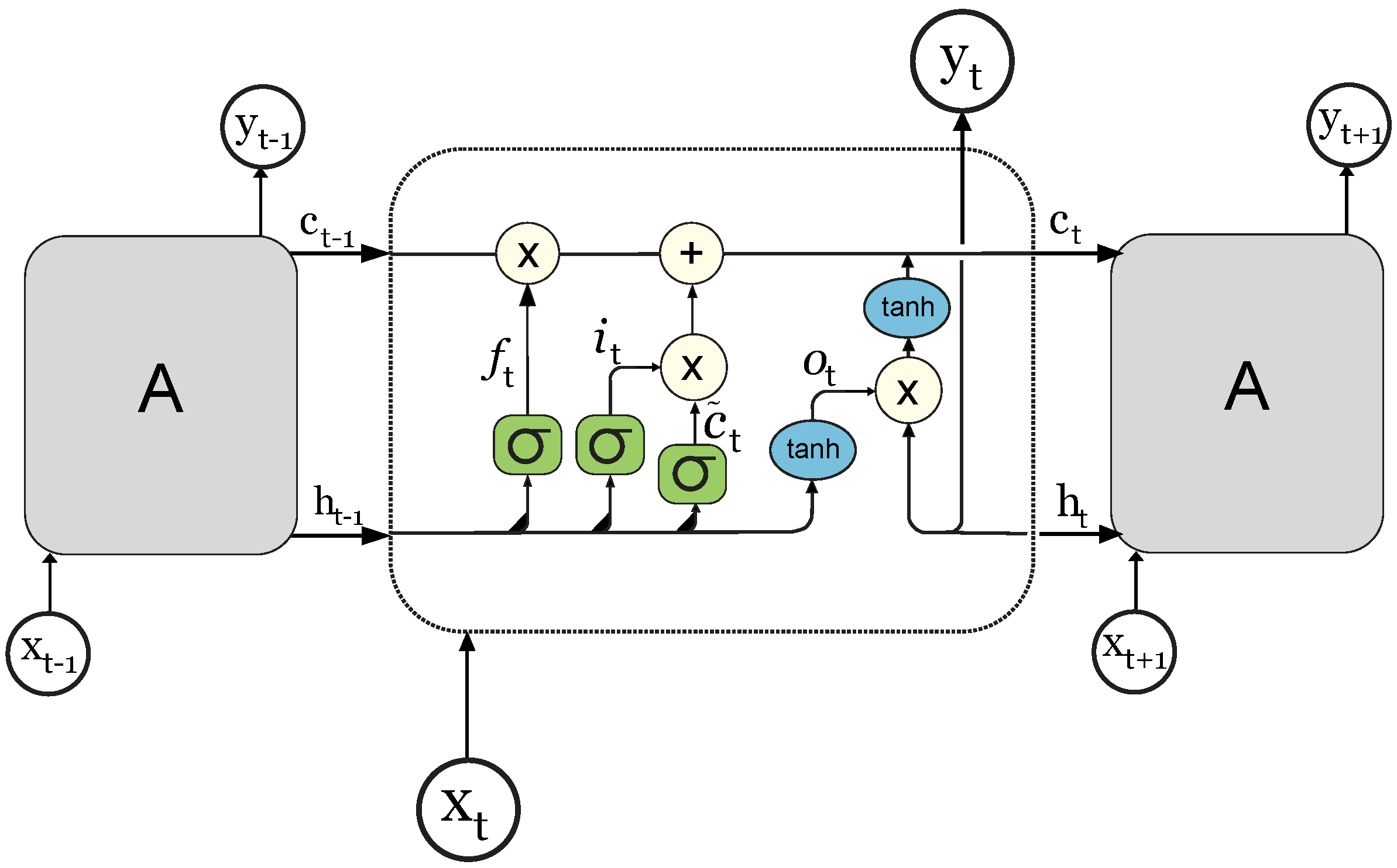
2.2. LSTM Architecture

LSTM is a form of multi-layer RNN which was developed by Hochreiter and Schmidhuber to help deal with the vanishing gradients problem [2,12,14]. The vanishing gradients problem refers to error signals vanishing during conventional backpropagation; the tendency to vanish arises from overly long learning time, which yields time lags between relevant inputs [2,14]. Moreover, there is the issue of older inputs being “forgotten” by the network as time steps increase with previous RNN configurations [2,14]. One of the key features of LSTM networks is the uninterrupted gradient flow, which can be thought of as a gradient highway, as opposed to the backpropagation of gradients which is present in classic RNNs [12]. LSTM achieves this through the implementation of a cell state $c_t$, which is an internal state that provides (in combination with the four internal gates) the ability to remove or add information and address long-lasting reliances [2,12]. The four aforementioned gates are the input, forget, output, and gate gate.

$$\left(\begin{array}{c}i\\ f\\ o\\ \tilde{c}\end{array}\right)=\left[\begin{array}{c}\sigma \\ \sigma \\ \sigma \\ tanh\end{array}\right]w^l\left(\begin{array}{c}{h}_t^{l-1}\\ h_{t-1}^l\end{array}\right)$$

(6)

where i, f, o, and $\tilde{c}$ are the input, forget, output, and gate gate, respectively [12]. Note that each gate has a different associated nonlinearity, such as a sigmoid function ($\sigma$) or hyperbolic tangent (tanh) [12]. $b_k$ and $w_k$ where $k\in i,f,o,g$ is the bias and weight matrices, respectively, and correspond to the associated gate [5,12].

$$\left(\begin{array}{c}{i}_t\\ f_t\\ o_t\\ {\tilde{c}}_t\end{array}\right)=\left[\begin{array}{c}\sigma (w_i[h_{t-1},x_t]+b_i)\\ \sigma (w_f[h_{t-1},x_t]+b_f)\\ \sigma (w_o[h_{t-1},x_t]+b_o)\\ tanh(w_c[h_{t-1},x_t]+b_c)\end{array}\right]$$

(7)

To begin the forward pass, the forget gate f is the first, and determines which information is kept; the previous hidden state $h_{t-1}$ and current input $x_t$ are concatenated and then go through this gate which is calculated by Equation (7) [12]. The sigmoid function provides an output between 0 and 1 for each element in $c_t$, where 1 indicates keep completely and 0 is erase completely [12]. Next, the input gate determines which value to update; once again $h_{t-1}$ and $x_t$ and inputs to calculate the gate as in Equation (7), with 1 meaning update completely, and 0 ignore completely [12]. Subsequently, the gate gate creates candidate values for the cell state via Equation (7) [12]. Due to the hyperbolic tangent, the output from this gate is a number between −1 and 1 for each element to be added to $c_t$ [12]. The cell state is updated by erasing data from it as determined by the forget gate, and then the new values are added as determined by the gate gate; the mathematical formulation is shown as [12]:

$$c_t=f_t\odot c_{t-1}+i_t\odot {\tilde{c}}_t$$

(8)

where ⊙ refers to Hadamard product (element-wise product). Next is the output gate which produces the output $y_t$ from the cell state [12]. This is determined by using the $h_{t-1}$ and $x_t$ once again to output a number between 0 and 1 for each element which must be revealed from the cell state to the output $y_t$, as shown in Equation (7) [12].

Finally, the hidden state is updated as dictated by the output gate and updated cell state and passed through a hyperbolic tangent to limit the values between −1 and 1, which is calculated as [12]:

$$h_t=o_t\odot tanh\left(c_t\right)$$

(9)

As previously stated, Figure 2 is a representation of the internal structures outlined [12]. Considering the backwards pass, the backpropagation from $c_t$ to $c_{t-1}$ is only elementwise multiplication by the forget gate, and does not involve multiplication by the weight matrix as in traditional RNNs [12].

The presented walkthrough of the forward pass and mechanisms allow the LSTM network to remember previous inputs from multiple time steps prior—which is vital for a sequential/time-series problem [2,12,13]. Moreover, the hyperbolic tangent function can provide quicker convergence than an analogous process with a non-symmetric activation function (such as a sigmoid function) [2]. The backwards pass uses a loss-optimization function which is set by the user; most often in literature for LSTM networks, this is designated as the adaptive moment estimation (ADAM) [2,5,9]. The ADAM algorithm minimizes total loss by updating the weights and biases of the network as indicated by the gradient of the loss function [2,9]. Note that during training, a single epoch refers to one or more batches, with each batch consisting of a forwards and backwards pass [2]. The training process continues through batches while the forwards and backwards passes continually update the network until a convergence or validation criteria are met [2,12].

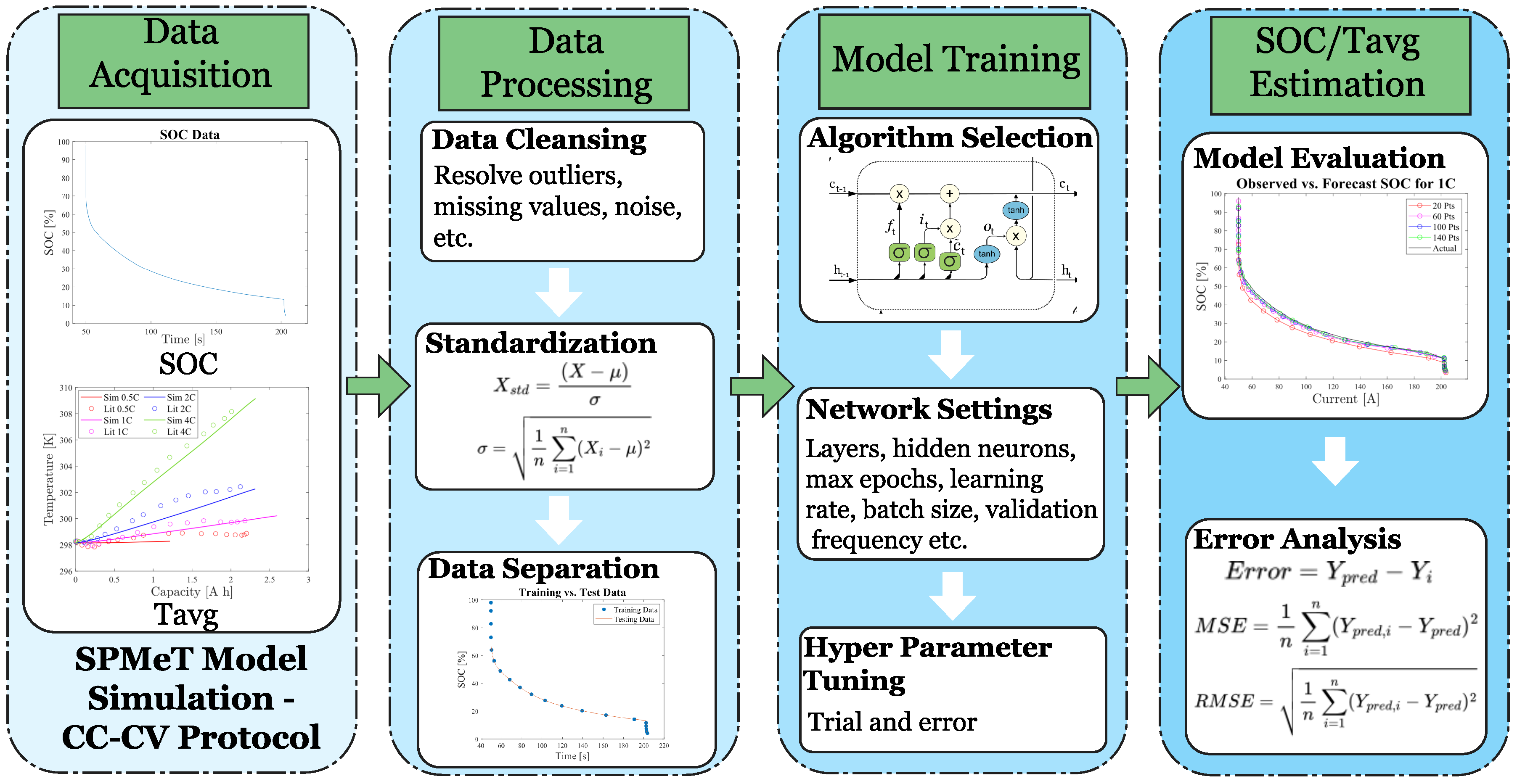
2.3. The Proposed LSTM-Based State-Estimation Method

An overview of the workflow for machine learning-based state estimation is illustrated in Figure 3. The process consists of four main modules: data acquisition, data processing, model training, and estimation of state-of-charge (SOC) and averaged temperature. In the first stage, the SPMeT model developed in [17] is simulated to generate reference SOC and temperature data. The data-processing module includes data cleaning, standardization, and partitioning into training and testing sets. An LSTM model is then trained to estimate SOC and temperature based on the processed data. Finally, the trained model is evaluated on the test dataset using mean squared error (MSE) and root mean squared error (RMSE) as performance metrics.

Choosing the inputs/features and outputs/responses for an ML problem is one of the most important and challenging issues [12]. For the purposes of this paper, the SOC and average cell temperature were chosen as the responses to the network. SOC was selected as it is one of the most significant battery health indicators and is of utmost interest to manufacturers, BMS usage, and more [2,5,6,9]. Meanwhile, average cell temperature was chosen due to its significance in contributing to degradation, safety implications, and ensuring high efficiency in charging/discharging procedures [10,15,29,30]. In this work, the average temperature is defined as the sum of core and surface temperatures divided by two, as posed by Perez et al. [19]. The input into the algorithm in this work was the applied current, with four different C-Rates considered (0.5C, 1C, 2C, and 4C). This choice is the most logical as it is what is applied to charge a battery in practice, and is the input into the electrochemical–thermodynamic model developed in the previous work [1]. However, an examination of the implementation of a multi-input single-output (MISO) network was completed, where the current, voltage, and capacity were taken as inputs. With the resulting network, it is much more complex to ensure acceptable results; cross-validation checks were implemented with five folds total, as well as dropout layers for regularization and to prevent overtraining, and two layers of hidden units as opposed to one (containing 100 hidden units each). The dropout layers have a rate of 20% [2]. To elaborate, the purpose of the cross-validation was to determine the optimal amount of training data versus testing data; in this instance, the validation data used were a portion of the training data to ensure the testing data remained unseen by the algorithm before testing [9]. In contrast, the single-feature designation was evaluated at varying amounts of training data to enable a more in-depth investigation. The multi-feature configuration performs sufficiently, but it has a much longer run time (approximately a minute longer in total) when compared to the single-input single-output configuration. Nonetheless, it was of great interest to examine this option, and it does provide greater flexibility for included features and improved generalizability of the model [9].

The specification of network hyperparameters plays an important role in the effectiveness of the state-estimation method. Table 1 and Table 2 summarize the hyperparameters used in this study, along with those reported in related literature. For the hyperparameters for SOC estimation, a default initial learning rate of 0.01 and the use of the ADAM optimizer are common choices. However, other hyperparameters, particularly the number of training epochs, show substantial variation across studies. The maximum number of epochs ranges from 150 to 3000 in previous works [2,5,6,9]. In the case of temperature estimation, the only consistent hyperparameter observed is the optimizer, with ADAM again being the preferred choice [10,11,15,30]. As with SOC, significant variation in epoch settings is noted, ranging from 8 to 5000 [10,11,15,30]. The selection of the maximum number of epochs is especially important, as it requires a careful trade-off between computational cost and the risk of overfitting [2,9]. Based on these findings, the hyperparameters used for SOC and temperature estimation in this study are detailed in Table 1 and Table 2, respectively.

3. Results

This section contains the state-estimation results from the LSTM network and is organized into five subsections: data separation, SOC estimation, temperature estimation, estimation using multiple inputs, and estimation using noisy data.

3.1. Data Generation

A new extended single-particle battery model (described by partial differential equations) coupled with thermal dynamics (described by ordinary differential equations), named SPMeT, has been developed in our recent work [17]. The model is validated with experiment data from literature and has shown great potential for efficient and high-fidelity simulations. In this section, we have used the proposed SPMeT model for data generation under varying current loads.

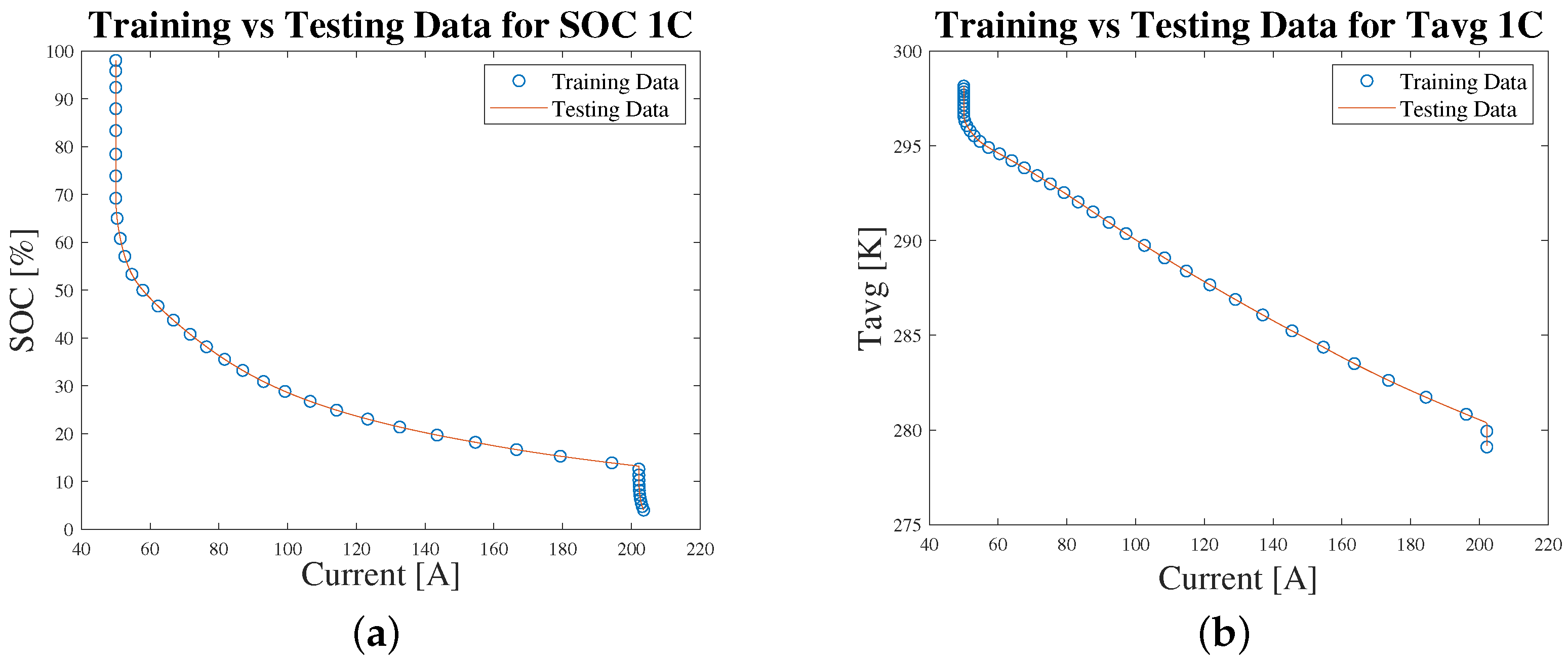
3.2. Data Separation

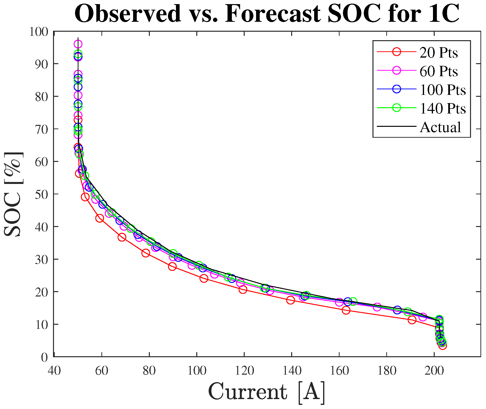
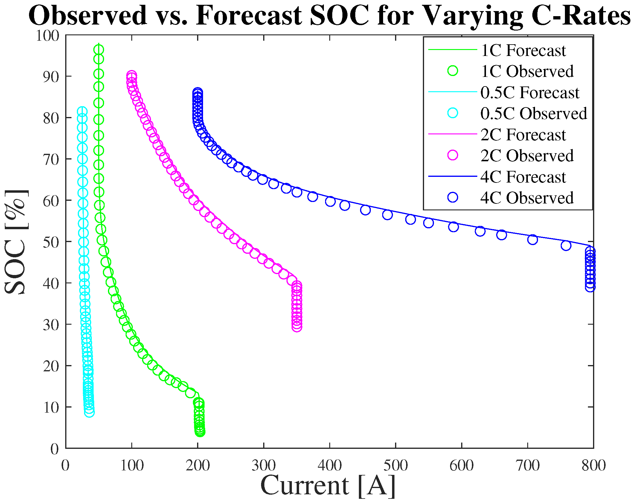
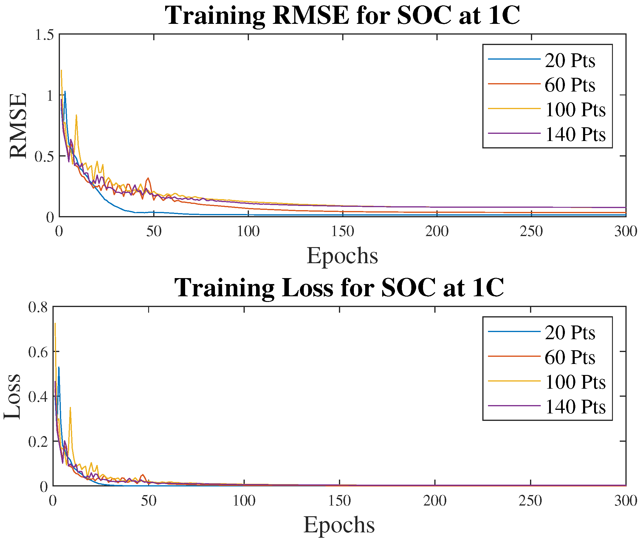
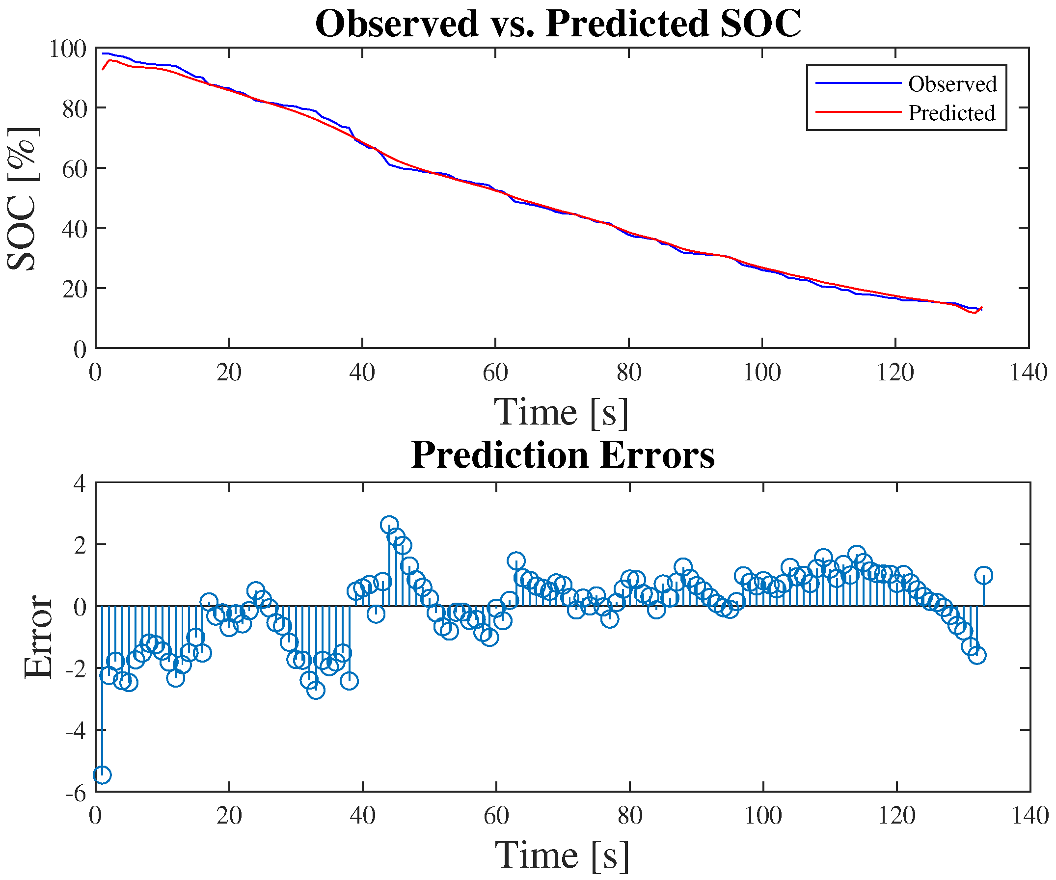
Two figures showing the two different methods for data partitioning examined in this work are presented; the evenly spaced training data with 40 points, and the first 70% of data for training (as is traditional) for the multiple-input configuration are depicted for both SOC and Tavg in Figure 4 and Figure 5, respectively. To ensure the validity of the model and provide a comprehensive analysis, both separation methods were used, where the primary format is shown in Figure 4, and the method in Figure 5 is used as verification.

3.3. SOC Estimation

Figure 6 shows the observed versus forecast values of SOC for varying amounts of training data at 1C. From Figure 6, one can see that the prediction performance is reasonably good in different cases, and as more points are used, better prediction performance is obtained. Meanwhile, a similar figure shows these results for multiple C-Rates instead in Figure 7. As can be seen in Figure 6, as the number of training data points increases, the algorithm predicts closer to the actual data; this is as expected. Moreover, the LSTM results in Figure 7 are promising, with the forecast values increasing in accuracy as the C-Rate decreases. Comparing the error values of the separation methods, there is a slight increase in error when applying traditional data partitioning but it is negligible. To be specific, for the 1C case, the customary approach yielded an RMSE of 2.504%, MSE of 6.270%, MAE of 0.454%, and PCC of 0.9934. Meanwhile, the corresponding values for the primary form of data separation are shown in

Table 4. Evaluation metrics for SOC estimation.

Evaluation Metrics—SOC
C-Rate	Training Points	RMSE (K)	MSE (K)	MAE (%)	PCC
0.5	20	4.166	17.356	3.732	0.9991
	60	1.372	1.881	1.226	0.9999
	100	0.835	0.696	0.735	0.9999
	140	0.894	0.800	0.561	0.9996
1	20	5.461	29.817	4.728	0.9991
	60	1.826	3.334	1.581	0.9999
	100	1.913	3.658	1.050	0.9986
	140	2.564	6.576	0.857	0.9965
2	20	3.206	10.276	3.136	0.9995
	60	1.054	1.110	1.022	0.9999
	100	0.669	0.447	0.617	0.9999
	140	0.950	0.903	0.480	0.9991
4	20	2.473	6.117	2.435	0.9997
	60	1.118	1.251	0.854	0.9987
	100	1.017	1.035	0.544	0.9982
	140	0.995	0.989	0.405	0.9980

; where the RMSE of the standard data separation is lower than the training results using 20 and 140 training points. Therefore, we have verified that the method of evenly spaced data partitioning across the entire dataset is valid for training.

The training progress is illustrated in Figure 8, and features the RMSE and loss throughout training. While lower amounts of training results exhibit smoother curves for training progress, the overall values are typically higher. This is supported by the evaluation metrics shown in Table 4.

Lastly, Figure 9 displays the error distribution for SOC for varying C-Rates. While the higher C-Rates show lower error values, they exhibit higher frequencies of such errors; consequently, this generally yields a tighter distribution of errors as the C-Rate increases. For predictions with a 4C-Rate, the most frequent error range is between 0 and $-1$%.

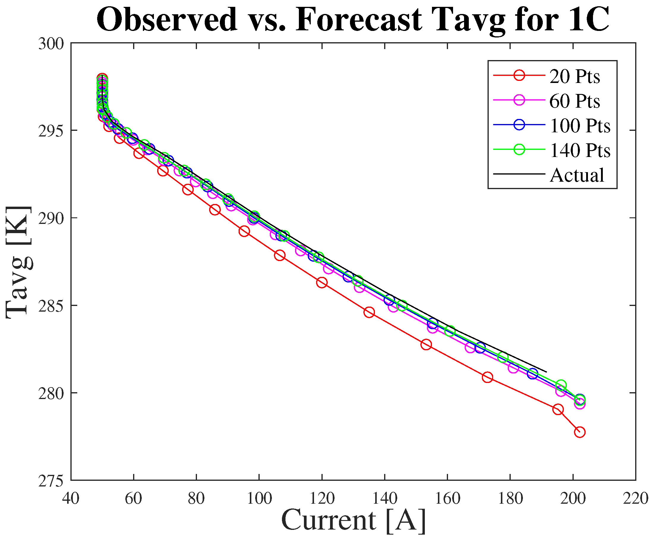
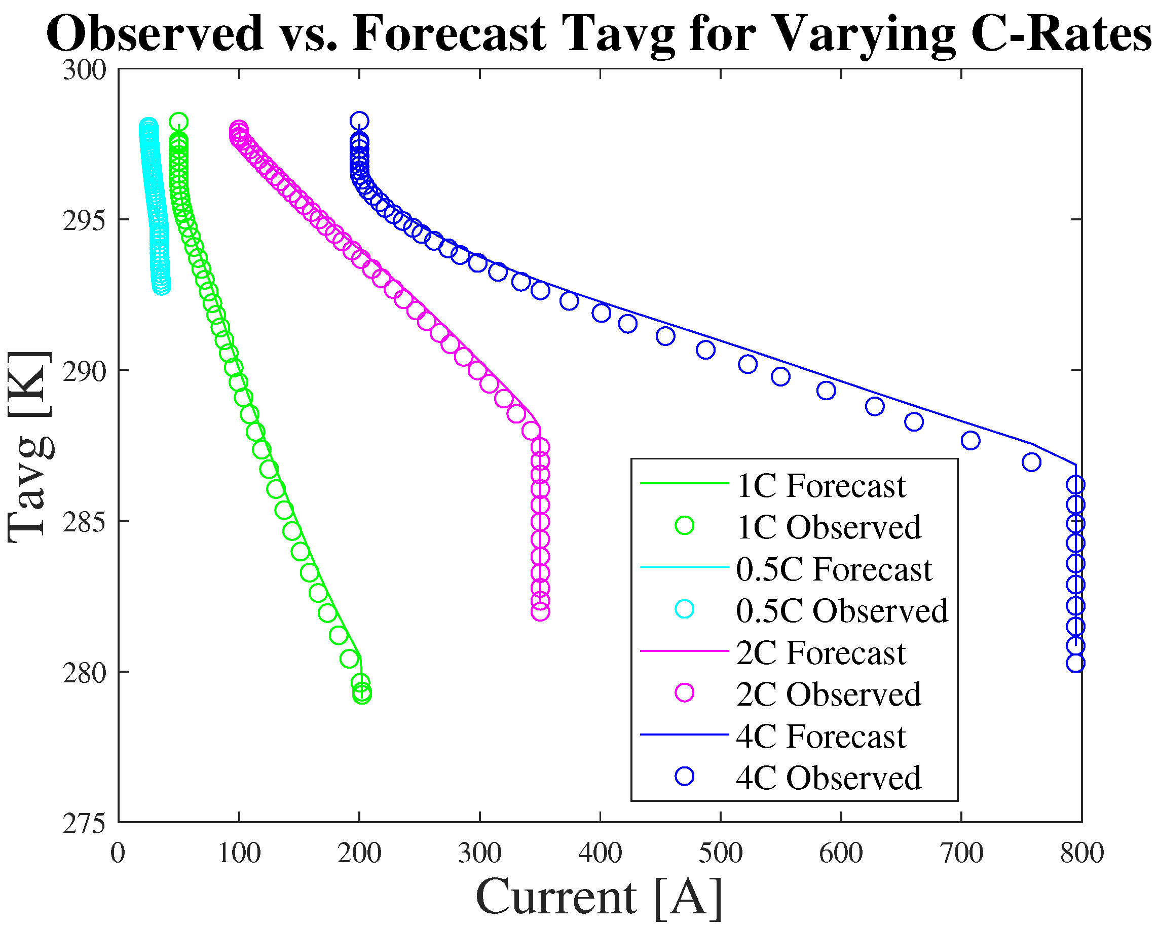
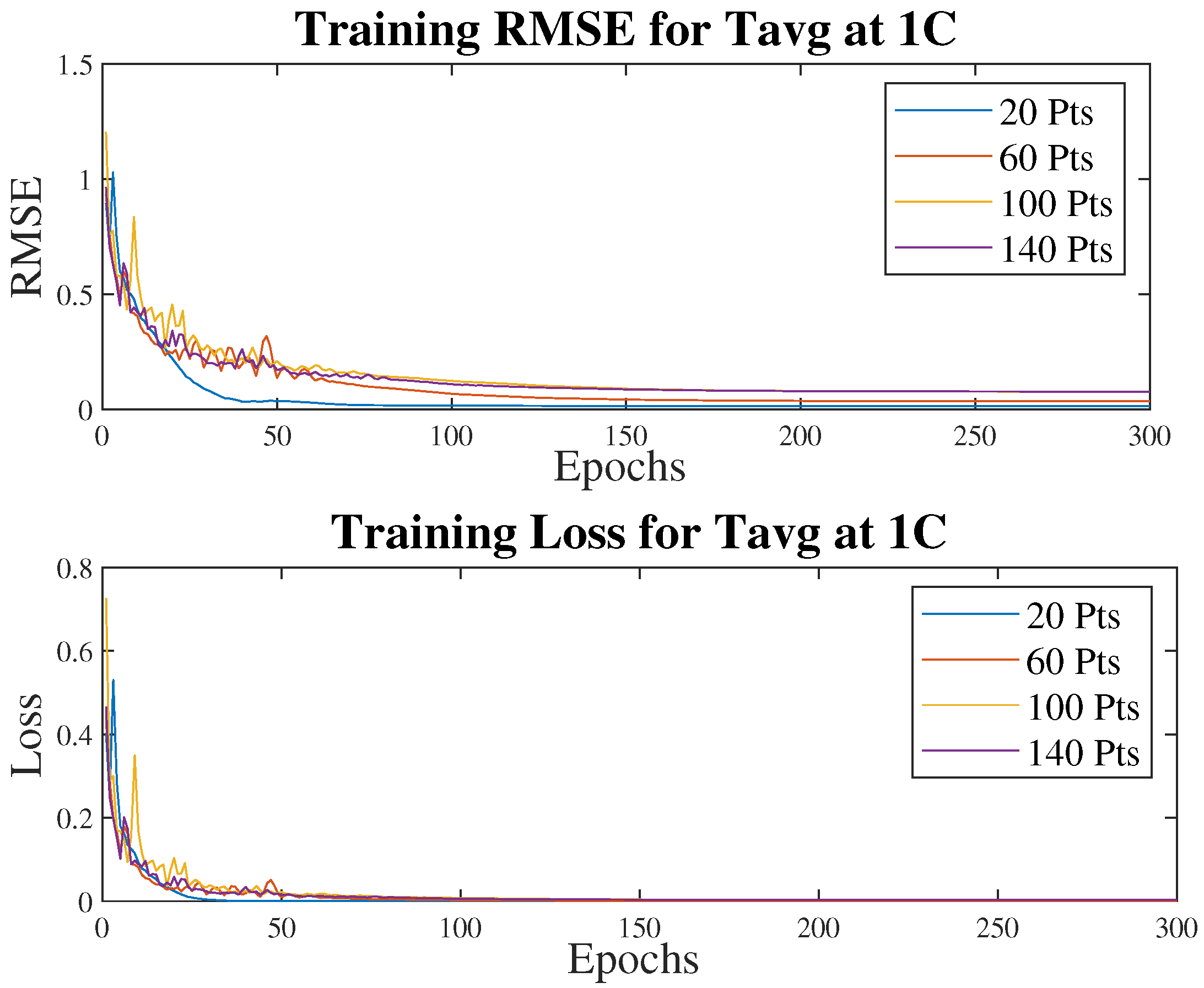
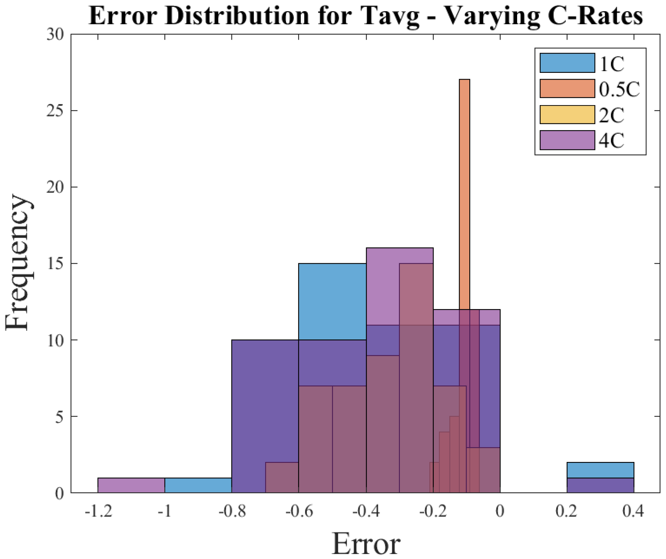
3.4. Temperature Estimation

Once again, Figure 10 illustrates the observed versus forecast values of Tavg for varying amounts of training data for 1C conditions. Similarly to the trends in Figure 6, as the number of training points increases the algorithm yields predictions closer to the actual values.

Concurrently to Figure 7, Figure 11 features the observed versus predicted values for varying C-Rates. Once again it is discerned that as C-Rate increases, the resulting forecast values stray further from the associated observed data.

The training progress, namely the RMSE and loss development, is shown in Figure 12 as a function of epochs. While decreasing the amount of training data yields a smoother curve, again the overall errors are larger. This is supported by

Table 5. Evaluation metrics for Tavg estimation.

Evaluation Metrics—Tavg
C-Rate	Training Points	RMSE (K)	MSE (K)	MAE (%)	PCC
0.5	20	0.311	0.097	0.296	0.9993
	60	0.092	0.009	0.090	0.9999
	100	0.059	0.004	0.055	0.9999
	140	0.063	0.004	0.041	0.9995
1	20	1.174	1.377	1.038	0.9990
	60	0.383	0.147	0.315	0.9995
	100	0.257	0.066	0.192	0.9996
	140	0.238	0.057	0.143	0.9995
2	20	0.963	0.927	0.872	0.9998
	60	0.301	0.091	0.269	0.9999
	100	0.259	0.067	0.170	0.9992
	140	0.239	0.057	0.119	0.9990
4	20	1.136	1.292	0.982	0.9995
	60	0.380	0.144	0.307	0.9994
	100	0.317	0.100	0.195	0.9989
	140	0.298	0.089	0.144	0.9987

, which shows the evaluation metrics for varying C-Rates and training points for Tavg.

Figure 13 shows the error distribution for the average cell temperature training for varying C-Rates. Interestingly, the figure shows an opposite trend to that in Figure 9; instead, as the C-Rate decreases so does the spread of errors, while the frequency increases. This is likely a result of the data the algorithm is trained on—given that the settings for each C-Rate remained the same and the plot contains data using runs from the same amount of training data. The results in Table 5 also mirror this observation. For 0.5 C-Rate settings, the most frequent error ranged from 0 K to −0.2 K.

3.5. Estimation Using Multiple Inputs

Figure 14 depicts the observed versus forecasted values for the SOC estimation with multiple features as the input. Additionally, the prediction error evolution is depicted in Figure 14 as well. As the settings of the network were altered to complete these simulations there are some differences in the results when compared to Figure 6. The increased resolution of data (decreasing downsampling factor) yields a less smooth curve for the observed values. Moreover, the distribution of the prediction errors is more widely spread, with the highest errors occurring at the beginning of the simulation.

The evaluation metrics are as follows:

• RMSE = 1.54
• MSE = 2.370
• MAE = 0.257
• PCC = 0.994

These metrics demonstrate improved accuracy compared to the results reported for the 1C-Rate SOC simulations in Table 4. Specifically, the prediction error metrics (including RMSE, MSE, and MAE values) are lower than those observed in the SISO case, while the PCC value remains comparable. This is expected as the associations between multiple features and one output are much more varied than those of a single feature and single output.

Meanwhile, the same set of figures is also depicted for the average cell temperature in Figure 15. The observed curve is once more less smooth due to the increased resolution of data (reduced downsampling factor). In contrast to Figure 14, the highest errors are at the end of the simulation. The evaluation of the MISO configuration for Tavg delivered the errors and PCC as:

• RMSE = 0.346
• MSE = 0.120
• MAE = 0.148
• PCC = 0.9984

Similar to the SOC estimation case, the comparison between single-input and multi-input cases for average temperature estimation shows superior predictive performance for the MISO configuration compared to the results shown in Table 5. This improvement is particularly evident when the number of training samples is limited to approximately 60 or fewer. For instance, at 60 training points, the RMSE achieved with the MISO model is 0.383 K, which is slightly higher than the 0.346 K obtained using the optimized single-input network. Additionally, the MAE remains comparable or lower across all cases with different numbers of training points, indicating that the multi-input architecture consistently provides improved accuracy. Moreover, the PCC value of 0.9984, although slightly lower than those in the SISO case, aligns with the expected trade-offs introduced by the increased complexity of mapping multiple input features to a single output. These findings suggest that MISO configurations offer a more effective modelling framework for both SOC and Tavg, particularly when training data is limited.

While there is increased accuracy overall with multiple features included in the network, the tradeoff is model complexity and run-time. Depending on the application of the network, either configuration could be appropriate as both show promising results in short run time.

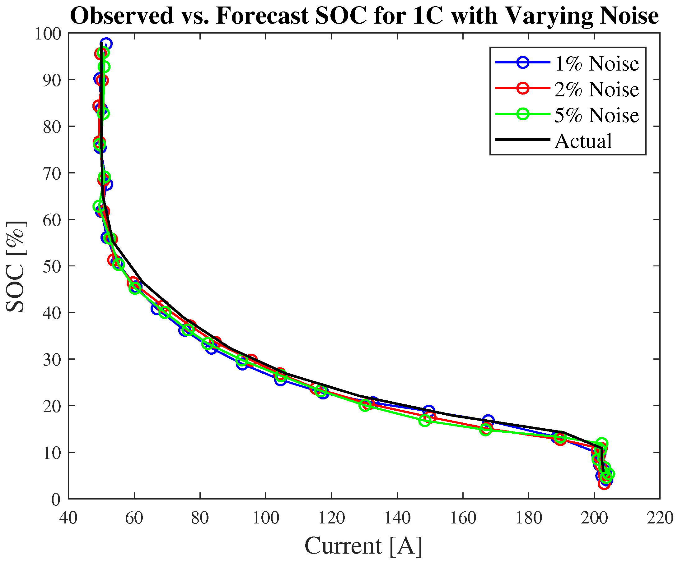
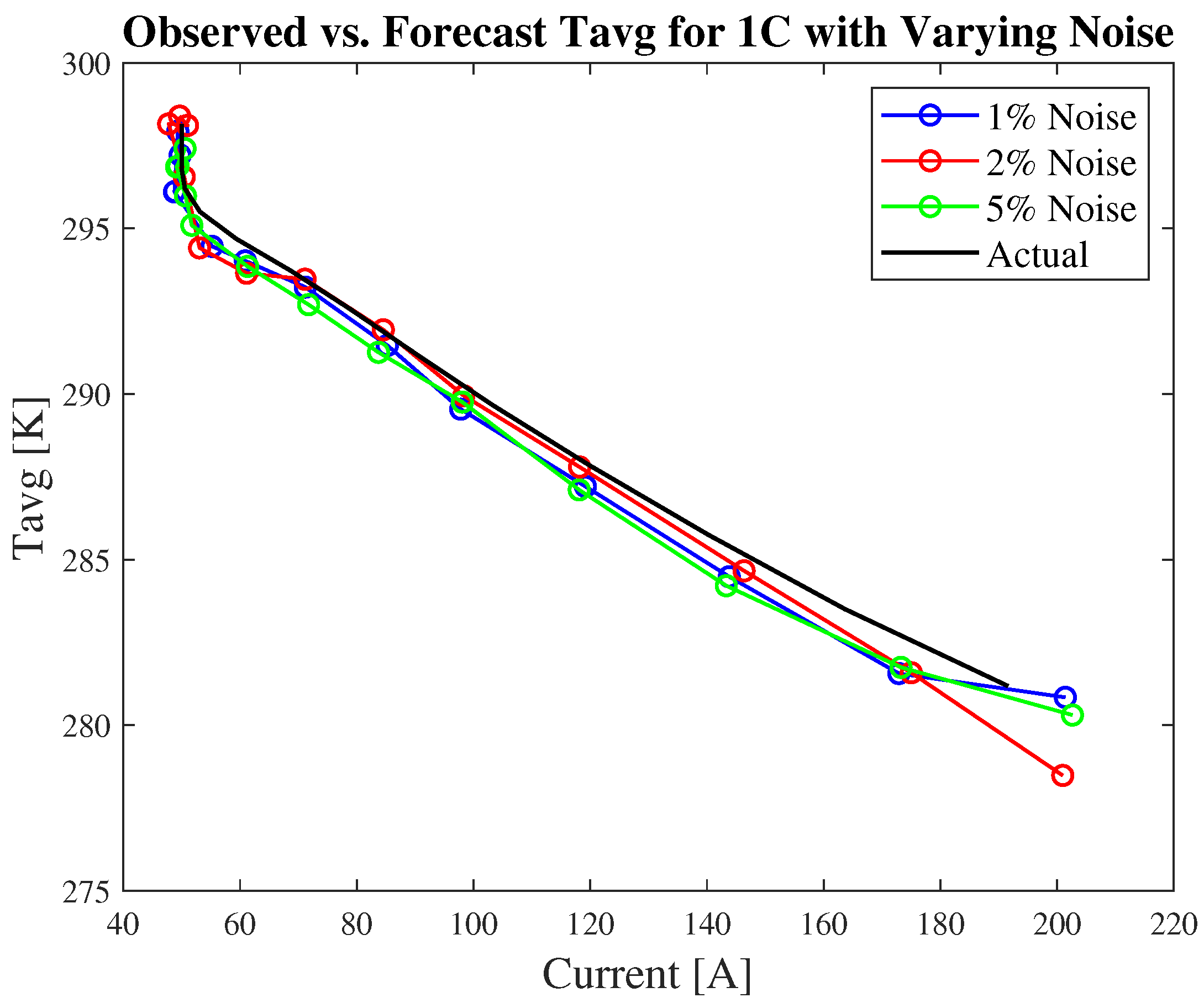
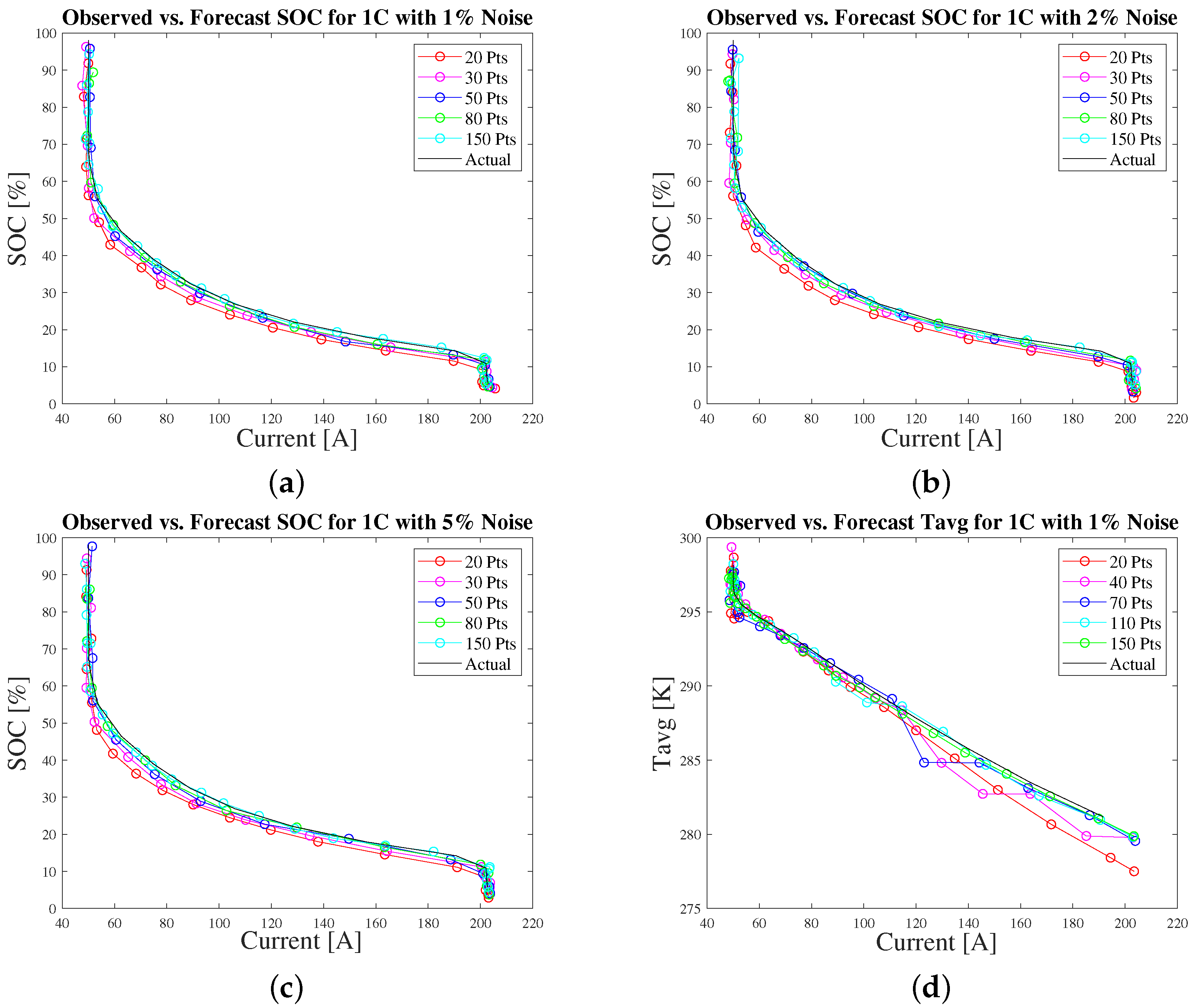
3.6. Estimation Using Noisy Data

To include the effect of noise on the simulations, the white Gaussian noise function in Matlab was used, where the input is the array representing applied current and SOC. The noise is termed “white” because it is spectrally flat (uniform energy distribution) across the entire sampling bandwidth [31]. Similarly, Du et al. also applied similar methods in verifying an ECM model performance with online parameter identification and noise interference [32]. A variance of 8 mA² was considered, which is approximately 0.8% of the highest value for the input current [32]. Meanwhile, for this work, a variance of 1.0% is used for noise generation on the input current. Another instance demonstrating the effect of noise on practical LIB application can be found in Lin et al.’s work [33]. In the test discharge experiments, the maximum noise set value used in the SOC estimation approach was 0.002 [33]. In terms of sampling frequency, this parameter varies widely in the industry and also depends on what type of measurement is taking place. For example, a simple thermocouple typically has a sampling time of 0.2 s, but this value increases with more advanced instruments. Given that the noise in the current work has a uniform distribution, the sampling time is comparable to this value. Moreover, one example of a minimum sampling frequency for a BMS is 50 Hz, meaning 50 samples considered per second [34].

Figure 16 presents a comparison between observed and forecasted SOC values under varying noise levels (1%, 2%, and 5%) at a 1C discharge rate. As shown in the figure, the prediction results remain generally accurate across the different noise levels. While a gradual degradation in prediction performance is observed with increasing noise, the overall impact on model accuracy remains limited. The predicted curves largely follow the observed trend, indicating that the network maintains robust performance even under moderate noise conditions.

Moreover, the observed versus forecast data are shown for deviating noise quantities in Figure 17. The effect of noise is much more obvious in Figure 17 than Figure 16. The simulations with 1 and 2% noise show some correctional behaviors at lower amounts of training data, where much larger deviations are noted for the 5% noise setting. Nonetheless, when 110 training points or more are used, the inclusion of noise appears to have very little influence on the accuracy of the algorithm.

Another foremost assessment of machine learning networks is the speed of convergence, which can be considered by the epoch at which the validation criteria are met [2,12]. In the simulations of the SOC at varying C-Rates, this occurs at approximately epoch 150 or prior, with decreased amounts of training data resulting in quicker convergence (as seen in Figure 18). A similar result is observed in examining the results of the Tavg simulations as illustrated in Figure 18.

Overall, the estimation of SOC using the single-feature configuration produces satisfactory results with RMSE values for all C-Rates using 60 training points or more ranging between 0.669–1.826%, and MAE between 1.581–0.405%. Additionally, all correlation values are above 0.99. The results of the average internal cell temperature are also sufficient. Values of RMSE for all C-Rates and all training points are between 0.059 K and 1.174 K, MSE between 0.004 K and 1.377 K, and MAE ranging from 0.041 to 1.038%. The PCC values also indicate a strong correlation with values above 0.99 for all cases. The issue of increased error at higher SOC values is also present in the literature, as shown in [2].

4. Conclusions

This paper developed an LSTM-based approach for estimating the SOC and average temperature of lithium–ion batteries under different current loads, using synthetic data generated by a previously established SPMeT model. The contributions of this paper are as follows: (1) The proposed method contributes a reliable and accurate data-driven framework for real-time battery state estimation. (2) The proposed method enhances the generalizability of model-based estimation while preserving essential physical insights. The influence of using multiple features in the network versus a single feature was examined, demonstrating the effectiveness of the MISO format for enhanced prediction accuracy. Additionally, the study evaluated the impact of different data-partitioning strategies, providing validation for the robustness of the proposed method. The performance of the model was evaluated based on RMSE, MSE, MAE, and the PCC. The key findings of this paper include the following: (1) The values of RMSE and MAE for SOC are typically below 1.5% for all C-Rates. Even stronger performance is shown by the network when estimating average internal cell temperature, with RMSE and MAE values below 1%. (2) The MISO format produced overall more accurate predictions while the network required to yield such results was much more complex and had a longer run time. (3) These metrics demonstrate that the network produces very accurate SOC and temperature estimations in suitable run time for real-time applications.

Some possible extensions to this work would be to apply the network to estimate the concentration of Li–ions as a spatial-temporal state by using the structure of the SPMeT model. The approach in the current manuscript leverages the resulting machine learning model as a surrogate through which much faster simulations of battery charging can take place. However, some challenges can arise and lead to errors when applying this method to a practical system. Foremost is a potential mismatch in parameters, battery type, or charging protocol. Given that these areas vary widely in battery research and application, this is very likely and could lead to errors in state estimation. To address this, future work should explore the integration of additional physico-chemical models, incorporation of heterogeneous battery systems, and investigation of hybrid model configurations. Moreover, the robustness of the model will be tested using experimental data from real batteries. An additional consideration for future studies is from the work of Sitapure and Kwon, wherein an LSTM controller is proposed [35]. The robust time series prediction capabilities of LSTM were utilized to allow for the prediction of future inputs via evaluation of state evolution from the current and previous time steps [35]. This framework provides an exciting avenue for advancement in BMS development.

References

1. Planella, F.B.; Ai, W.; Boyce, A.M.; Ghosh, A.; Korotkin, I.; Sahu, S.; Sulzer, V.; Timms, R.; Tranter, T.G.; Zyskin, M.; et al. A continuum of physics-based lithium–ion battery models reviewed. Prog. Energy 2022, 4, 042003. [Google Scholar] [CrossRef]
2. Yang, F.; Zhang, S.; Li, W.; Miao, Q. State-of-charge estimation of lithium–ion batteries using LSTM and UKF. Energy 2020, 201, 117664. [Google Scholar] [CrossRef]
3. Yi, Y.; Xia, C.; Feng, C.; Zhang, W.; Fu, C.; Qian, L.; Chen, S. Digital twin-long short-term memory (LSTM) neural network based real-time temperature prediction and degradation model analysis for lithium–ion battery. J. Energy Storage 2023, 64, 107203. [Google Scholar] [CrossRef]
4. Khah, M.V.; Zahedi, R.; Eskandarpanah, R.; Mirzaei, A.M.; Farahani, O.N.; Malek, I.; Rezaei, N. Optimal sizing of residential photovoltaic and battery system connected to the power grid based on the cost of energy and peak load. Heliyon 2023, 9, e14414. [Google Scholar] [CrossRef] [PubMed]
5. Chen, J.; Zhang, Y.; Wu, J.; Cheng, W.; Zhu, Q. SOC estimation for lithium–ion battery using the LSTM-RNN with extended input and constrained output. Energy 2023, 262, 125375. [Google Scholar] [CrossRef]
6. Yang, F.; Li, W.; Li, C.; Miao, Q. State-of-charge estimation of lithium–ion batteries based on gated recurrent neural network. Energy 2019, 175, 66–75. [Google Scholar] [CrossRef]
7. Chung, D.; Ko, J.; Yoon, K. State-of-Charge Estimation of Lithium–ion Batteries Using LSTM Deep Learning Method. J. Electr. Eng. Technol. 2022, 17, 1931–1945. [Google Scholar] [CrossRef]
8. Zhang, C.; Li, K.; Deng, J. Real-time estimation of battery internal temperature based on a simplified thermoelectric model. J. Power Sources 2016, 302, 146–154. [Google Scholar] [CrossRef]
9. Zhao, F.; Guo, Y.; Chen, B. A Review of Lithium–Ion Battery State of Charge Estimation Methods Based on Machine Learning. World Electr. Veh. J 2024, 15, 131. [Google Scholar] [CrossRef]
10. Cho, G.; Zhu, D.; Campbell, J.J.; Wang, M. An LSTM-PINN Hybrid Method to Estimate Lithium–Ion Battery Pack Temperature. IEEE Access 2022, 10, 100594–100604. [Google Scholar] [CrossRef]
11. Yao, Q.; Lu, D.D.; Lei, G. A Surface Temperature Estimation Method for Lithium–Ion Battery Using Enhanced GRU-RNN. IEEE Trans. Transp. Electrif. 2023, 9, 1103–1112. [Google Scholar] [CrossRef]
12. Li, F.; Krishna, R.; Xu, D. Lecture 10: Recurrent Neural Networks. 2021. Available online: https://cs231n.stanford.edu/2021/slides/2021/lecture_10.pdf (accessed on 7 January 2025).
13. Yin, W.; Kann, K.; Yu, M.; Schütze, H. Comparative Study of CNN and RNN for Natural Language Processing. arXiv 2017, arXiv:1702.01923. [Google Scholar] [CrossRef]
14. Hochreiter, S. The Vanishing Gradient Problem During Learning Recurrent Neural Nets and Problem Solutions. Int. J. Uncertain. Fuzziness Knowl.-Based Syst. 1998, 6, 107–116. [Google Scholar] [CrossRef]
15. Jiang, Y.; Yu, Y.; Huang, J.; Cai, W.; Marco, J. Li–ion battery temperature estimation based on recurrent neural networks. Sci. China Technol. Sci. 2021, 64, 1335–1344. [Google Scholar] [CrossRef]
16. Wang, L.; Luo, F.; Xu, Y.; Gao, K.; Zhao, X.; Wang, R.; Pan, C.; Liu, L. Analysis and estimation of internal temperature characteristics of Lithium–ion batteries in electric vehicles. Ind. Eng. Chem. Res. 2023, 62, 7657–7670. [Google Scholar] [CrossRef]
17. Chevalier, B.; Xie, J.; Dubljevic, S. Enhanced Dynamic Modeling and Analysis of a Lithium–Ion Battery: Coupling Extended Single Particle Model with Thermal Dynamics. 2024; under review. [Google Scholar]
18. Xie, J.; Dubljevic, S. Discrete-time Kalman filter design for linear infinite-dimensional systems. Processes 2019, 7, 451. [Google Scholar] [CrossRef]
19. Perez, H.E.; Dey, S.; Hu, X.; Moura, S.J. Optimal Charging of Li-Ion Batteries via a Single Particle Model with Electrolyte and Thermal Dynamics. J. Electrochem. Soc. 2017, 164, A1679. [Google Scholar] [CrossRef]
20. Roman, D.; Saxena, S.; Robu, V.; Pecht, M.; Flynn, D. Machine learning pipeline for battery state-of-health estimation. Nat. Mach. Intell. 2021, 3, 447–456. [Google Scholar] [CrossRef]
21. Danko, M.; Adamec, J.; Taraba, M.; Drgona, P. Overview of batteries State of Charge estimation methods. Transp. Res. Proc. 2019, 40, 186–192. [Google Scholar] [CrossRef]
22. Richardson, R.; Ireland, P.; Howey, D.; Richardson, R.; Ireland, P.; Howey, D. Battery internal temperature estimation by combined impedance and surface temperature measurement. J. Power Sources 2014, 265, 254–261. [Google Scholar] [CrossRef]
23. Bhadriraju, B.; Kwon, J.S.I.; Khan, F. An adaptive data-driven approach for two-timescale dynamics prediction and remaining useful life estimation of Li–ion batteries. Comput. Chem. Eng. 2023, 175, 108275. [Google Scholar] [CrossRef]
24. Hwang, G.; Sitapure, N.; Moon, J.; Lee, H.; Hwang, S.; Sang-Il Kwon, J. Model predictive control of Lithium–ion batteries: Development of optimal charging profile for reduced intracycle capacity fade using an enhanced single particle model (SPM) with first-principled chemical/mechanical degradation mechanisms. Chem. Eng. J. 2022, 435, 134768. [Google Scholar] [CrossRef]
25. Lee, H.; Sitapure, N.; Hwang, S.; Kwon, J.S.I. Multiscale modeling of dendrite formation in lithium–ion batteries. Comput. Chem. Eng. 2021, 153, 107415. [Google Scholar] [CrossRef]
26. Sitapure, N.; Kwon, J.S.I. Exploring the potential of time-series transformers for process modeling and control in chemical systems: An inevitable paradigm shift? Chem. Eng. Res. Des. 2023, 194, 461–477. [Google Scholar] [CrossRef]
27. Shi, Y.; Ahmad, S.; Tong, Q.; Lim, T.M.; Wei, Z.; Ji, D.; Eze, C.M.; Zhao, J. The optimization of state of charge and state of health estimation for lithium-ions battery using combined deep learning and Kalman filter methods. Int. J. Energy Res. 2021, 45, 11206–11230. [Google Scholar] [CrossRef]
28. Li, M.; Li, C.; Zhang, Q.; Liao, W.; Rao, Z. State of charge estimation of Li–ion batteries based on deep learning methods and particle-swarm-optimized Kalman filter. J. Energy Storage 2023, 64, 107191. [Google Scholar] [CrossRef]
29. Chen, Y.; Kang, Y.; Zhao, Y.; Wang, L.; Liu, J.; Li, Y.; Liang, Z.; He, X.; Li, X.; Tavajohi, N.; et al. A review of lithium–ion battery safety concerns: The issues, strategies, and testing standards. J. Energy Chem. 2021, 59, 83–99. [Google Scholar] [CrossRef]
30. Naguib, M.; Kollmeyer, P.; Vidal, C.; Emadi, A. Accurate Surface Temperature Estimation of Lithium–Ion Batteries Using Feedforward and Recurrent Artificial Neural Networks. In Proceedings of the 2021 IEEE Transportation Electrification Conference & Expo (ITEC), Chicago, IL, USA, 21–25 June 2021; pp. 52–57. [Google Scholar] [CrossRef]
31. Marmarelis, V.Z. Appendix II: Gaussian White Noise. In Nonlinear Dynamic Modeling of Physiological Systems; John Wiley & Sons, Ltd.: Hoboken, NJ, USA, 2004; pp. 499–501. [Google Scholar]
32. Du, X.; Meng, J.; Liu, K.; Zhang, Y.; Wang, S.; Peng, J.; Liu, T. Online Identification of Lithium–ion Battery Model Parameters with Initial Value Uncertainty and Measurement Noise. Chin. J. Mech. Eng. 2023, 36, 7. [Google Scholar] [CrossRef]
33. Lin, L.; Kawarabayashi, N.; Fukui, M.; Tsukiyama, S.; Shirakawa, I. A Practical and Accurate SOC Estimation System for Lithium-Ion Batteries by EKF. In Proceedings of the 2014 IEEE Vehicle Power and Propulsion Conference (VPPC), Coimbra, Portugal, 27–30 October 2014; pp. 1–6. [Google Scholar] [CrossRef]
34. Su, X.; Sun, B.; Wang, J.; Zhang, W.; Ma, S.; He, X.; Ruan, H. Fast capacity estimation for lithium–ion battery based on online identification of low-frequency electrochemical impedance spectroscopy and Gaussian process regression. Appl. Energy 2022, 322, 119516. [Google Scholar] [CrossRef]
35. Sitapure, N.; Kwon, J.S.I. Machine learning meets process control: Unveiling the potential of LSTMc. AIChE J. 2024, 70, e18356. [Google Scholar] [CrossRef]
36. The MathWorks Inc. Statistics and Machine Learning Toolbox; The MathWorks Inc.: Natick, MA, USA, 2022; Available online: https://www.mathworks.com/help/stats/index.html (accessed on 7 January 2025).
Figure 1. General RNN configuration—unrolled [12].
Processes 13 01528 g001
Figure 2. LSTM internal diagram [5,12].
Processes 13 01528 g002
Figure 3. State estimation overview.
Processes 13 01528 g003
Figure 4. Data separation—evenly spaced for 1C; (a) training vs. testing data for SOC; (b) training vs. testing data for Tavg.
Processes 13 01528 g004
Figure 5. Data separation—traditional format for 1C; (a) training vs. testing data for SOC; (b) training vs. testing data for Tavg.
Processes 13 01528 g005
Figure 6. Observed vs. forecast 1C.
Processes 13 01528 g006
Figure 7. Observed vs. forecast all C-Rates.
Processes 13 01528 g007
Figure 8. Training progress.
Processes 13 01528 g008
Figure 9. Error distribution.
Processes 13 01528 g009
Figure 10. Observed vs. forecast 1C.
Processes 13 01528 g010
Figure 11. Observed vs. forecast all C-Rates.
Processes 13 01528 g011
Figure 12. Training progress.
Processes 13 01528 g012
Figure 13. Error distribution.
Processes 13 01528 g013
Figure 14. MISO configuration results for 1C—SOC.
Processes 13 01528 g014
Figure 15. MISO configuration results for 1C—Tavg.
Processes 13 01528 g015
Figure 16. SOC observed vs. forecast with varying noise levels.
Processes 13 01528 g016
Figure 17. Tavg observed vs. forecast with varying noise levels.
Processes 13 01528 g017
Figure 18. SOC and Tavg estimation using noisy data for varying training data points.
Processes 13 01528 g018aProcesses 13 01528 g018b