Predicting Indirect Tensile Strength of Rejuvenated Asphalt Mixes Using Machine Learning with High Reclaimed Asphalt Pavement Content

Abstract

Predicting the performance of hot mix asphalt (HMA) is crucial for ensuring pavement durability, especially as the use of rejuvenated reclaimed asphalt pavement (RAP) increases in sustainable construction. Indirect tensile strength (ITS) is a critical parameter that indicates a pavement’s resistance to cracking and distress under traffic loads. This study developed statistical and machine learning models—linear regression, support vector machine (SVM), and artificial neural network (ANN)—to predict ITS and ITS loss in RAP-incorporated HMA rejuvenated with waste cooking oil (WCO) and waste engine oil (WEO). The models used key input variables, including rejuvenator type and the composition of asphalt, rejuvenator, and RAP. Results showed that WCO increased initial ITS, while WEO enhanced durability by reducing ITS loss. Additionally, lower RAP and asphalt content contributed to improved pavement durability. Among the predictive models, ANN demonstrated the highest accuracy, exhibiting lower error metrics and less variation in scatterplots compared to regression and SVM models. The only exception was ITS loss percentage prediction, where the mean absolute error was nearly identical across all models. These predictive models provide valuable insights for designing and testing modified asphalt mixtures, particularly those containing RAP. By optimizing mix design and enabling proactive maintenance strategies, they contribute to the development of more durable and sustainable pavement infrastructure with the provision of accurate and workable models for prediction of ITS and loss prediction which can be used for design.

1. Introduction

Reclaimed asphalt pavement (RAP), obtained from recycling the top layer of old pavements, is used in new asphalt concrete for reducing the need for new materials and minimizing waste in roadway construction. In recent years, the use of RAP in road construction has drawn significant attention as a viable replacement for natural aggregate and binder in flexible pavement. However, the use of a higher percentage of RAP results in several concerns related to the performance and subsequent service life of asphalt pavement. One of the main challenges of using RAP in bituminous mixtures stems from the increased stiffness of aged pavement, posing a major challenge to its use in road construction. Without a softening treatment, RAP can make the mix excessively stiff and difficult to compact, potentially leading to premature pavement failure [1]. This increased stiffness results from progressive oxidation, which modifies asphalt components and degrades its viscoelastic properties [2]. The rigidity of RAP can be mitigated through methods such as warm mix technology, increased asphalt content, and the use of softer asphalt [3]. These approaches reduce stiffness by softening aged asphalt without altering its chemical composition. However, at higher RAP contents, these techniques become less effective or impractical. To sustainably meet the growing demand for road materials without compromising performance, RAP must be utilized efficiently. Rejuvenators have emerged as a reliable alternative for incorporating higher RAP content, as they replenish lost aromatic components in aged asphalt, restoring its chemical structure and reducing binder viscosity. Various commercial rejuvenators (CRs) are particularly recommended for RAP levels exceeding 30% [4]. In addition to CR, the use of waste materials as recycling agents has been found to be a sustainable solution and to promote an environmentally friendly approach to RAP utilization in road construction. The use of waste materials is also considered to a more cost-effective solution for pavement construction which needs large quantities of raw materials [5]. The use of waste materials as rejuvenators mitigates the issue of their disposal and reduces the need for commercial production of rejuvenators. The latter involves chemical processes which produce harmful impacts for the environment. Different kinds of waste material have been considered potential sources of recycling agents and can be found elsewhere [6]. The scope of the study is limited to the waste cooking oil (WCO) and the waste engine oil (WEO).

WEO and WCO, two different types of waste oil, have both been investigated as potential additives for asphalt mixtures by numerous studies [6,7,8,9,10,11,12,13,14]. These studies found that WCO and WEO could significantly change some asphalt mixture properties. Other earlier investigations concluded that using a significant amount of aromatic fractions or resin can have a stronger rejuvenating effect and proposed WEO and WCO based on different characteristics [15]. The majority of the essential physical and chemical features of bitumen are shared by WEOs, since both of them originate as a product of petroleum refinement. Due to its similarity to the molecular structures of asphalt with sufficient aromatic concentration, WEO modifies the components and revitalizes aged asphalt. However, till 2009, very few studies attempted to explore the potential of WEO as a rejuvenator. According to research conducted over the last ten years, WEO improves several properties, including low-temperature cracking [16], fatigue resistance [17], workability [18], and temperature sensitivity [19]. In addition to WEO, various kinds of edible vegetable oil, animal oil, and palm oil are utilized in frying and cooking processes, which produce significant amounts of WCO [20]. The organic acid component of WCO belongs to the family of cohesive agents [13]. RAP’s cohesive element reduces viscosity, reducing the binder’s surface tension. It also produces cohesion and removes the air curtain that encloses the aggregate. As a result, the addition of cohesive agents and new bituminous materials accelerates the development of homogeneous mixtures. While the addition of waste oil has been shown to enhance pavement performance, it may also reduce ductility and weaken the adhesion between aggregate and asphalt [21], potentially impacting Indirect Tensile Strength (ITS). Therefore, a thorough understanding of the effects of waste oil on the ITS of rejuvenated RAP asphalt mixtures is crucial, particularly when incorporating higher percentages of RAP.

The mechanical characteristics and resistance to distress of asphalt mixes incorporate two important parameters, the Indirect Tensile Strength (ITS) and ITS loss. Indirect tensile strength is a parameter which is used to measure the asphalt mix’s ability to withstand the shear failure which materializes in the form of rutting which is a commonly observed distress in flexible pavements [22]. ITS loss refers to the reduction in ITS of a wet sample compared to a dry sample. This parameter shows the pavement’s ability to withstand damage due to water accumulation. Developing a prediction model for ITS and ITS loss in RAP-incorporated HMA is essential for assessing pavement durability and performance. It enables early detection of distress, evaluates material quality, and predicts pavement lifespan, aiding in proactive maintenance and rehabilitation. Given the influence of traffic, environmental conditions, and material properties on ITS loss, such models help optimize mix designs and ensure long-term pavement sustainability. Unfortunately, none of the studies attempted to develop prediction models for ITS and ITS loss for RAP incorporated HMA mixtures rejuvenated by two such potential rejuvenating agents, WCO and WEO. The current models for prediction asphalt mix properties are empirical and do not provide the adaptability to be used in unique cases with non-traditional components [23]. Hence, the present study aimed to develop prediction models tailored for measuring ITS and ITS loss using statistical and machine learning techniques.

Researchers have studied methods for predicting and optimizing the ITS properties of RAP-containing rejuvenated asphalt mixtures through computational modeling. One approach simulates the behavior of asphalt mixtures under different loading and environmental conditions. Another method involves analyzing the properties of asphalt mixtures with varying RAP content and evaluating their field performance through experimental testing. Statistical methods have traditionally been used to predict the ITS characteristics of asphalt mixtures. Garrick and Biskur developed a regression model to examine the relationship between ITS and asphalt properties [23]. The study involved mixtures made with two types of aggregate (gravel and traprock) and 15 different asphalt types. A regression analysis indicated that, as ITS increased, penetration decreased. Additionally, the slope of the relationship between penetration and tensile strength varied significantly depending on the aggregate type. Another study explored the effect of RAP combined with waste high-density polyethylene on the indirect tensile stiffness modulus (ITSM) of asphalt concrete surfaces at different RAP contents [24]. The regression analysis revealed that ITSM increased with higher RAP content but decreased as the test temperature rose. Similarly, a regression model was used to optimize RAP content for each RAP size while ensuring the unconfined compressive strength (UCS) remained above the lower limit of 27.6 MPa [25]. The results showed that incorporating RAP led to reductions in ITS, UCS, and the elastic modulus. These studies have relied on statistical models and empirical data analysis to establish relationships between input variables and output responses. However, with the advent of machine learning, more advanced computational techniques have emerged, enabling the efficient processing of large datasets and the identification of complex patterns. The use of machine learning techniques, for the prediction of ITS and its loss of rejuvenated asphalt mixtures incorporating RAP, has been rarely found in the literature in which such a combination is attempted [26,27,28,29,30]. These studies compare the performance of statistical and machine learning methodologies for prediction of ITS and its loss. Previous studies have mainly employed analytical models, on standard asphalt mixes, for the prediction of ITS using stress parameters. This would be the first study in which machine learning techniques have been used to predict ITS and its loss for asphalt mixes with rejuvenation and high RAP content. The following objectives have been set for this study:

• Develop models for predicting ITS and ITS Loss for rejuvenated asphalt mixes with RAP.
• Compare the performance of statistical and machine learning techniques for prediction of ITS and ITS loss.

The previous literature shows a lack in the development and suggestion of workable models which can be used for optimizing mix design of asphalt mix with rejuvenated asphalt and high RAP content. Hence, this study aims to identify optimal modeling methods to predict ITS and ITS loss in rejuvenated asphalt mixtures with RAP concentration by contrasting and evaluating the efficacy of statistical and machine learning methodologies.

The remainder of this paper is divided into the following sections: Section 2 presents an overview of the modeling techniques used for the study. Section 3 describes the research approach adopted for experimental work. Results and discussions are provided in Section 4. Section 5 presents the comparison of developed models. The main conclusions of this study are finally outlined in Section 6, along with suggestions for additional research.

2. Modeling Techniques

Three types of modeling technique have been used in this study, namely, multivariate regression model, support vector machines (SVM), and artificial neural networks (ANNs). Regression models are statistical models that take the form of Equation (1) [31].

$$Y=a+f(\sum bx)$$

(1)

where Y is the output, a and b are the model coefficients, and x is the vector of input parameters. The coefficients are determined using ordinary least squares and accepted if they significantly impact the model, indicated by a t-value with a 5% probability threshold. SVMs are widely used for modeling discrete or pattern recognition data, and are increasingly applied to prediction problems [32]. They identify data samples that map to hyperplanes while maximizing their separation (as shown in Figure 1), known as support vectors [33,34,35].

Due to dataset complexity, input parameters are mapped using a kernel function, similar to regression (see Equation (2)).

$$Y=b+\alpha f(bias+\sum Wx)$$

(2)

where Y is the output parameter, b and $\alpha$ are the constants for the mapping function, and bias and W are the model coefficients for each support vector.

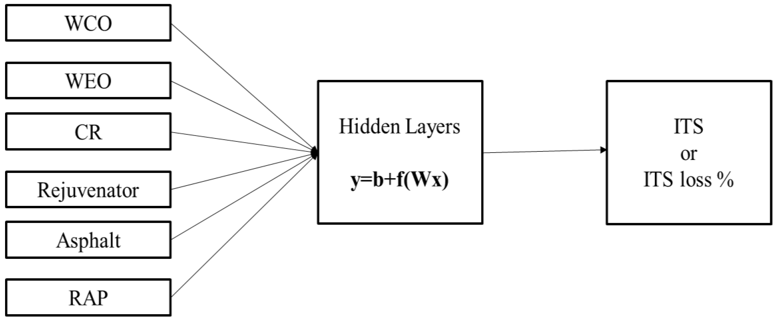
The ANN model is another popular branch of machine learning techniques, which is considered very efficient at predicting problems. This is mainly due to its generalization abilities for noisy data [36]. There are different types of ANN, such as multilayer feedforward (MLFF), radial basis function (RBF), and general regression neural network (GRNN) [34]. In this study, MLFF has been used due to their popularity among researchers and simpler architecture [37]. MLFF architecture is depicted in Figure 2, in which the variables used in this study have also been shown. It comprises three types of layer, namely, input, hidden, and output. The input layer feeds the network with the independent variables, which are moved forward to the hidden layer(s). The hidden layer comprises several neurons, each taking all the input values and processing them through an activation function after estimating weights and bias. The processed quantity is moved forward to the next hidden layer (if there is any) or the output layer, which takes these quantities and processes them to give the final output. The predicted output is compared with the actual values and the sum of the square of errors is used to update the weights and biases of the network [38].

There can be several parameters of MLFF architecture which affect its accuracy, such as the number of hidden layers and hidden neurons in each layer, activation function, learning algorithm, etc. It is virtually impossible to determine the optimum combination of these parameters without fixing any of them [39]. This is due to the large number of parameters involved in the training of MLFNN, resulting in infinite combinations which are practically impossible to compare completely. Hence, the activation functions for the hidden layer were set as hyperbolic while that for the output layer was set as a logistic, which is shown in Equations (3) and (4) [40]. The activation functions transform the outputs from the previous layers, with the use of estimated weights, and provide outputs for the model or the proceeding layer. Conjugate gradient and backpropagation learning algorithms were used. The maximum number of hidden layers was set at 2, while the maximum number of hidden neurons in each layer was set at 11. The optimum values of hidden layers, neurons, and their associated weights were found by trying all possible combinations within the given ranges and then selecting the combination with the highest accuracy.

$$h={\displaystyle \frac{e^x-e^{-x}}{e^x+e^{-x}}}$$

(3)

$$l=1/(1+e^{-x})$$

(4)

3. Research Approach

3.1. Materials

The study utilized aggregates from Dammam, and asphalt from the Ras Tanura oil refinery. All relevant properties of the binder, aggregate, and RAP were evaluated according to standard procedures and met the requirements set by the Ministry of Transport and Logistical Support (MOTLS), Saudi Arabia. To achieve the desired final gradation and volumetric properties, finer fractions of virgin aggregate were combined with coarse RAP, ensuring compliance with specified standards. Three RAP levels—30%, 40%, and 50%—were used to achieve the target gradation. The viscosity of the RAP binder, in the presence of a specific rejuvenator, was determined using the blending chart [41]. Based on the established correlation, incorporating 20% waste oil by weight of the total reclaimed binder resulted in a viscosity comparable to that of new asphalt. To evaluate the rejuvenator’s effects, this percentage was systematically adjusted by ±7%. The optimal asphalt content for fresh mixtures was 6.1%, while for mixtures containing 30%, 40%, and 50% RAP, the values were 5.5%, 5.2%, and 5.0%, respectively.

3.2. Laboratory Testing

The specimens were prepared in line with the specification and standard based on the optimal asphalt level calculated by the Marshall mix design for various testing. Figure 3 shows the experimental setup for the testing. Two different tests were carried out for the study. The tensile property of asphalt pavement is a crucial variable determining cracking behavior, which can be successfully measured using the ITS test. According to ASTM D6931, the ITS value is determined at a controlled temperature of 25 °C by subjecting a cylindrical sample (101 mm in diameter) to continual tensile stress (51 mm/min) along the diametrical axis until failure occurs using the following equation:

$$ITS=P_{max}/(3.1416\times H\times D)$$

(5)

Here, “P_max” represents the maximum applied force, while “H” and “D” reflect the specimen’s height and diameter, respectively. The ITS loss was evaluated following AASHTO T283. To determine the degree of moisture damage, samples were prepared and divided into two subsets, each containing three specimens. One subset was tested in dry conditions at room temperature, while the other was conditioned by immersing samples in water at 60 °C for 24 h, followed by 2 h at 25 °C, before being brought to the test temperature for wet tensile strength measurement. The tensile strength ratio (TSR) was then calculated using the following equation:

$$\mathrm{\%}ITSloss={ITS}_{wet}/{ITS}_{dry}$$

(6)

Here, ITS_wet and ITS_dry represent the indirect tensile strengths of wet and dry samples, respectively.

3.3. Experimental Design

The rejuvenated mixtures incorporating waste oil were evaluated using two key tests: ITS and percentage loss in ITS. Each test was conducted in triplicate, resulting in a total of 225 samples. The rejuvenator type, rejuvenation percentage, and the proportions of RAP and asphalt varied across the samples. For WCO and WEO, rejuvenation percentages of 13%, 20%, and 27% were used, while the standard rejuvenator was applied at 7% and 13%. The optimum asphalt content for RAP percentages of 30%, 40%, and 50% was determined to be 5.5%, 5.2%, and 5.0%, respectively. In comparison, the control sample had an optimum asphalt content of 6.1%. To assess the impact of binder content on the mechanical and volumetric properties of asphalt mixtures, the optimal asphalt content was adjusted by ±0.5%. The plan is shown in Figure 4.

3.4. Modeling Methodology

The available dataset was divided into training and test samples, wherein the former was used for model development and the latter for testing the accuracy of the model. A total of 2 out of 3 samples for each combination were randomly taken for training (i.e., 67% of the dataset), and the remaining were kept for testing dataset. Therefore, there was at least one sample for each combination of variables tested in this study to avoid any biases in the accuracies. The accuracy for each model was calculated using mean absolute error (MAE) and mean absolute percentage (MAPE) for training and test datasets. Moreover, scatter plots were also made between predicted and tested outputs to see the graphical presentation of the fit between these two datasets.

Each of the modeling methods employs a different method for optimization of parameters. In the case of the regression model, the method of partial least squares was used to optimize the coefficients and weights. For machine learning models, the training data were further sub-divided into two sets using a 2:1 approach for training and cross-validation, respectively. The squared error term was used to compare the performance of models with different hyperparameters. The hyperparameters for SVM included the weights, bias, and constants for the support vectors. In addition, a dual learning mechanism was applied to ANN models for optimizing the hyperparameters including hidden layers and neurons.

4. Results and Discussion

The regression model developed for predicting ITS is shown in Equation (7), while that for ITS loss % is shown in Equation (8). The model fitness parameters are shown in

Table 1. ITS Multiple linear regression.

Parameter	Value for ITS Prediction Model	Value for ITS Loss % Prediction Model
Multiple R	0.81	0.82
Multiple R2	0.65	0.67
Adjusted R2	0.64	0.66
Sum of Squares Model	739,798	5010
Degrees of Freedom Model	5	6
Mean Sum of Squares Model	147,960	835
Sum of Squares Residual	395,844	2450
Degrees of Freedom Residual	144	143
Mean Sum of Squares Residual	2749	17
F	54	49
p	0	0

, while the scatterplots are plotted in Figure 5, which show the comparison of observed and predicted values for the training and test datasets. Figure 6 shows the comparison of accuracy parameters calculated for the regression models for training and test datasets.

Each type of rejuvenator was taken as a dichotomous dummy variable in the model. Equation (7) shows that type of rejuvenators increases the tensile strength with the highest increase observed for WCO, shown by its coefficient which is the highest for the model. These results conform to those of previous studies, such as Ziari et al. [42]. This impact is attributed to the rejuvenator’s molecular interaction with asphaltene molecules in RAP [43]. RAP content did not have a significant effect on the model which could be due to its range, and a wider range may show a significant impact on the model. Rejuvenator content has a negative impact on ITS. The model presented by Equation (8) shows that all rejuvenator types decrease the loss in ITS with the highest effect (coefficient) due to WEO, in addition to asphalt content. This could be attributed to the molecular interaction of these rejuvenators, as stated above. Moreover, RAP and rejuvenator content increase the loss in ITS, hence, it could be said that using them in lower proportions increases the durability of asphalt mix. The previous studies have attributed such behavior to the loss in viscosity of these asphaltic items due to their ageing [44]. Table 1 shows that both models had a statistically significant F-statistic (p-value = 0), which confirms that the regression models can capture significant variation in the data.

ITS = 509 + 236(WCO) + 94(WEO) + 125(Standard) + 36(Asphalt%) − 12(Rejuvenator%)

(7)

ITS Loss = 49.7 − 24.6(WCO) − 29.3(WEO) − 22.9(Standard) − 5.5(Asphalt%) + 0.3(RAP%) + 0.5(Rejuvenator%)

(8)

Figure 5a,b show a wide spread of the scatterplot for training and test datasets. Figure 6a shows that MAE increases by 20 kPa and MAPE increases by 5% for the test dataset as compared to training data, while predicting ITS using a regression model. On the other hand, there is no significant change in MAE for the ITS loss prediction model (Figure 6b) between test and training samples, while an approximately 50% increase in MAPE is shown for test samples of this model, compared to the training dataset.

Table 2. SVM for ITS prediction.

Parameter	Value for ITS Prediction Model	Value for ITS Loss % Prediction Model
Number of independents	6	6
SVM type	Regression	Regression
$\alpha$	0.1	0.1
B	0.17	0.17
Kernel type	Radial Basis Function	Radial Basis Function
Number of SVMs	104	114

shows the parameters for SVM models for ITS and ITS loss % prediction while the weights for this model are provided in Appendix A. The kernel function used was the radial basis function, which gave the best accuracy. There are no restrictions for the significance of any parameter, hence, all six parameters were used as an input for the model. Figure 7 shows the scatterplots for the predicted values while error values are shown in Figure 8. A total number of 104 samples were identified from the training dataset as the support vectors for the ITS prediction model, while 114 of them were found as support vectors for the ITS loss % prediction model. The number of support vectors in this problem are considerable large which makes the model computationally problematic and inappropriate for optimization of parameters [45].

Figure 7 shows a close spread of the predicted values with very few values (for training and test datasets) in the middle range having a high prediction for ITS (Figure 7a). Figure 8a presents an increase of approximately 15 KPa in MAE and 5% in MAPE for the test dataset compared to training samples. Figure 8b shows a negligible change in MAE (%) and a 50% increase in MAPE for test samples of the ITS loss prediction model, compared to training samples. The R² value for the ITS prediction model was very low for the test dataset, and significantly different from the training dataset which is an indication of overfitting issue [46].

Parameters for ANN models are presented in

Table 3. ANN model for ITS prediction.

Parameter	Value for ITS Prediction Model	Value for ITS Loss % Prediction Model
Hidden layers	2	2
Hidden neurons	11, 8	6, 8
Hidden layer activation function	Hyperbolic
Output layer activation function	Logistic
Learning algorithm	Back propagation, Conjugate gradient

, while the scatterplot and error values for these models are shown in Figure 9 and Figure 10, respectively. Appendix B contains the values for the weights of neurons in the ANN model. Two hidden layers were required in both these models to have maximum accuracy. The number of hidden neurons in the first layer was eleven for ITS prediction, while those for ITS loss prediction were 6. The second hidden layer in both cases had 8 neurons. The number of hidden layers can enable accurate predictions for complex problems [47], such as the one at hand in this case which has multiple variables with unknown impacts. However, increasing the number of layers to a high number can have a large impact on processing time. In this regard, hidden layers equal to or less than 3 are considered appropriate [47]. The dual learning approach, which has been adopted in this study for training the neural networks, was found to be helpful in previous studies to refine the results [48].

Figure 9a shows that only a couple of values from the middle range in the test dataset were predicted high by the model, while all other predicted values seem close to the observed data. Figure 9b shows that most of the test samples have a wider spread as compared to the training samples for ITS loss predictions. Figure 10a shows an increase of 25 KPa in MAE and 5% in MAPE for the test dataset in comparison to training samples. Figure 10b shows an increase of approximately 3% in MAE and 55% for MAPE for ITS loss predictions on test samples as compared to training samples.

All models have shown a high change in MAPE for ITS loss prediction while having a small change in MAE. This could be because ITS loss has a limited range (>1 and <100), hence, a small increase in its value results in a large increase in the percentage error.

5. Comparison of Models

All models were compared based on their error values obtained for the test samples for respective predictions. This comparison is presented in Figure 11. It can be observed from the figure that the ANN model outperforms others for ITS prediction. MAE for ITS loss % prediction was found to be approximately the same for all models, while MAPE for ANN was lowest for this case. Moreover, the SVM models’ performance was better than that of the regression models. Therefore, machine learning has proved to be a more accurate approach for prediction modeling in this study. This could be attributed to the free-forming structure of these models unlike the fixed form of regression models. Moreover, it could be concluded that ANN would be the best choice to predict ITS and its Loss % for rejuvenated asphalt mix with high RAP content. The ANN superiority for prediction modeling is largely attributed to its parallel processing structure employing multiple neurons for this purpose.

In the case of the error terms, there is an obvious impact of the variable (ITS or ITS loss %) on the error terms of MAPE and MAE. In the case of ITS values, MAPE seem to be more stable parameters, while in case of ITS loss % the error value of MAE is more stable. This could be attributed to the nature of the variable wherein ITS has a larger range and variability compared to ITS%. Hence, it is recommended that multiple error terms should be used for prediction modeling, and the selection of results should be based on the suitability of error term to the predicted variable.

6. Conclusions

This study was aimed at developing models for predicting ITS and ITS loss for rejuvenated asphalt mix with a high RAP content. Three types of technique were used for this purpose, namely, a linear regression model, SVM, and ANN. The type of rejuvenator and the content of asphalt, rejuvenator, and RAP were used as inputs in the model. The regression model showed that the use of WCO would increase the initial ITS for the mix, while the use of WEO can give better durability than other types of rejuvenator. Secondly, it was found that using the lower content of asphalt and RAP gives better durability. ANN performed better than the other models used in this study. The scatterplots for these models showed less variation compared to the other models. Moreover, error parameters for ANN models, except MAE for ITS loss % prediction, were lower than regression models and SVMs. MAE for ITS loss % was found to be approximately the same for all models. The models developed in this study would be useful for researchers involved with the design and testing of modified asphalt mixes, especially with RAP content. However, future research should expand experimental data with diverse variables to refine prediction models. Additionally, studies should assess long-term aging, economic and environmental impacts, alternative rejuvenators, and real-world validation for sustainable pavement development.

References

1. Odubela, C.A.; Yaacob, H.; Warid, M.N.B.M.; Karim, K.J.A.; Kamaruddin, N.H.B.M.; Al-Saffar, Z.H.; Rahim, M.I.K. Rheological and chemical properties of reclaimed asphalt pavement using polyethylene terephthalate (PET) additive as a modifier. Environ. Sci. Pollut. Res. 2025, 32, 8025–8034. [Google Scholar] [CrossRef]
2. Abouelsaad, A.; White, G. Review of Asphalt Mixture Ravelling Mechanisms, Causes and Testing. Int. J. Pavement Res. Technol. 2022, 15, 1448–1462. [Google Scholar] [CrossRef]
3. Santos, S.D.; Partl, M.N.; Poulikakos, L.D. From virgin to recycled bitumen: A microstructural view. Compos. B Eng. 2015, 80, 177–185. [Google Scholar] [CrossRef]
4. Liu, S.; Shukla, A.; Nandra, T. Technological, environmental and economic aspects of Asphalt recycling for road construction. Renew. Sustain. Energy Rev. 2017, 75, 879–893. [Google Scholar] [CrossRef]
5. Hasan, U.; Whyte, A.; Al Jassmi, H.; Hasan, A. Lifecycle cost analysis of recycled asphalt pavements: Determining cost of recycled materials for an urban highway section. CivilEng 2022, 3, 316–331. [Google Scholar] [CrossRef]
6. Rahman, M.T.; Mohajerani, A.; Giustozzi, F. Recycling of Waste Materials for Asphalt Concrete and Bitumen: A Review. Materials 2020, 13, 1495. [Google Scholar] [CrossRef]
7. Islam, M.K.; Gazder, U.; Al Mamun, A.; Arifuzzaman, M.; Al-Abdul Wahhab, H.I.; Rahman, M.M. Predicting and optimizing the mechanical properties of rejuvenated asphalt mix with RAP content. Neural Comput. Appl. 2024, 37, 2071–2087. [Google Scholar] [CrossRef]
8. Mamun, A.A.; Al-Abdul Wahhab, H.I. Comparative laboratory evaluation of waste cooking oil rejuvenated asphalt concrete mixtures for high contents of reclaimed asphalt pavement. Int. J. Pavement Eng. 2020, 21, 1297–1308. [Google Scholar] [CrossRef]
9. Al Mamun, A.; Al-Abdul Wahhab, H.I.; Dalhat, M.A. Comparative Evaluation of Waste Cooking Oil and Waste Engine Oil Rejuvenated Asphalt Concrete Mixtures. Arab. J. Sci. Eng. 2020, 45, 7987–7997. [Google Scholar] [CrossRef]
10. Mamun, A.A.; Al-Abdul Wahhab, H.I. Evaluation of Waste Engine Oil-Rejuvenated Asphalt Concrete Mixtures with High RAP Content. Adv. Mater. Sci. Eng. 2018, 2018, 7386256. [Google Scholar] [CrossRef]
11. Elkashef, M.; Podolsky, J.; Williams, R.C.; Cochran, E. Preliminary examination of soybean oil derived material as a potential rejuvenator through Superpave criteria and asphalt bitumen rheology. Constr. Build. Mater. 2017, 149, 826–836. [Google Scholar] [CrossRef]
12. Hugener, M.; Partl, M.N.; Morant, M. Cold asphalt recycling with 100% reclaimed asphalt pavement and vegetable oil-based rejuvenators. Road Mater. Pavement Des. 2014, 15, 239–258. [Google Scholar] [CrossRef]
13. Jia, X.; Huang, B.; Moore, J.A.; Zhao, S. Influence of Waste Engine Oil on Asphalt Mixtures Containing Reclaimed Asphalt Pavement. J. Mater. Civ. Eng. 2015, 27, 04015042. [Google Scholar] [CrossRef]
14. Li, Y.; Shen, A.; Lyu, Z.; Wang, S.; Formela, K.; Zhang, G. Ground tire rubber thermo-mechanically devulcanized in the presence of waste engine oil as asphalt modifier. Constr. Build. Mater. 2019, 222, 588–600. [Google Scholar] [CrossRef]
15. Zhang, J.; Sun, H.; Jiang, H.; Xu, X.; Liang, M.; Hou, Y.; Yao, Z. Experimental assessment of reclaimed bitumen and RAP asphalt mixtures incorporating a developed rejuvenator. Constr. Build. Mater. 2019, 215, 660–669. [Google Scholar] [CrossRef]
16. Liu, S.; Peng, A.; Wu, J.; Zhou, S.B. Waste engine oil influences on chemical and rheological properties of different asphalt binders. Constr. Build. Mater. 2018, 191, 1210–1220. [Google Scholar] [CrossRef]
17. Fernandes, S.; Peralta, J.; Oliveira, J.R.M.; Williams, R.C.; Silva, H.M.R.D. Improving Asphalt Mixture Performance by Partially Replacing Bitumen with Waste Motor Oil and Elastomer Modifiers. Appl. Sci. 2017, 7, 794. [Google Scholar] [CrossRef]
18. Qurashi, I.A.; Swamy, A.K. Viscoelastic properties of recycled asphalt binder containing waste engine oil. J. Clean. Prod. 2018, 182, 992–1000. [Google Scholar] [CrossRef]
19. Wang, F.; Fang, Y.; Chen, Z.; Wei, H. Effect of waste engine oil on asphalt reclaimed properties. AIP Conf. Proc. 2018, 1973, 020012. [Google Scholar] [CrossRef]
20. Villanueva, A.; Ho, S.; Zanzotto, L. Asphalt modification with used lubricating oil. Can. J. Civ. Eng. 2008, 35, 148–157. [Google Scholar] [CrossRef]
21. You, T.; Balamurugan, S.S.; Nazzal, M.D.; Mohammad, L.N.; Negulescua, I.; Daly, W.H. Rheological, Chemical, Micromechanical, and Mechanical Properties of Re-Refined Engine Oil Bottoms (REOB) Modified Binders. In Proceedings of the Transportation Research Board 97th Annual Meeting, Washington, DC, USA, 7–11 January 2018. [Google Scholar]
22. Nascimento, F.A.C.; Guimarães, A.C.R.; Castro, C.D. Comparative study on permanent deformation in asphalt mixtures from indirect tensile strength testing and laboratory wheel tracking. Constr. Build. Mater. 2021, 305, 124736. [Google Scholar] [CrossRef]
23. Garrick, N.W.; Biskur, R.R. Effects of Asphalt Properties on Indirect Tensile Strength. trid.trb.org. 1990. Available online: https://trid.trb.org/View/348912 (accessed on 13 March 2025).
24. Liu, J.; Liu, F.; Zheng, C.; Zhou, D.; Wang, L. Optimizing asphalt mix design through predicting effective asphalt content and absorbed asphalt content using machine learning. Constr. Build. Mater. 2022, 325, 126607. [Google Scholar] [CrossRef]
25. Aschuri, I.; Woodward, D. Modification of a 14mm asphalt concrete surfacing using RAP and waste HDPE plastic. Int. J. Pavements 2010, 9, 70–78. [Google Scholar]
26. Ahmadi, A.; Gogheri, M.K.; Adresi, M.; Amoosoltani, E. Laboratory evaluation of roller compacted concrete containing RAP. Adv. Concr. Constr. 2020, 10, 489–498. [Google Scholar]
27. Ozsahin, T.S.; Oruc, S. Neural network model for resilient modulus of emulsified asphalt mixtures. Constr. Build. Mater. 2008, 22, 1436–1445. [Google Scholar] [CrossRef]
28. Xiao, F.; Amirkhanian, S.N. Effects of Binders on Resilient Modulus of Rubberized Mixtures Containing RAP Using Artificial Neural Network Approach. J. Test. Eval. 2009, 37, 129–138. [Google Scholar] [CrossRef]
29. Islam, M.K.; Gazder, U.; Alam, M.S.; Shalabi, F.I.; Arifuzzaman, M. Behavioral Investigation of Single Wall and Double Wall CNT Mixed Asphalt Adhesion Force Using Chemical Force Microscopy and Artificial Neural Networks. Appl. Sci. 2022, 12, 2379. [Google Scholar] [CrossRef]
30. Kezhen, Y.; Yin, H.; Liao, H.; Huang, L. Prediction of Resilient Modulus of Asphalt Pavement Material Using Support Vector Machine. In Road Pavement and Material Characterization, Modeling, and Maintenance; ASCE: Reston, VA, USA, 2011; pp. 16–23. [Google Scholar] [CrossRef]
31. Horton, N.J.; Lipsitz, S.R. Review of Software to Fit Generalized Estimating Equation Regression Models. Am. Stat. 1999, 53, 160. [Google Scholar] [CrossRef]
32. Chen, C.H.; Peter Ho, P.G. Statistical pattern recognition in remote sensing. Pattern Recognit. 2008, 41, 2731–2741. [Google Scholar] [CrossRef]
33. Maalouf, M.; Khoury, N.; Trafalis, T.B. Support vector regression to predict asphalt mix performance. Int. J. Numer. Anal. Methods Geomech. 2008, 32, 1989–1996. [Google Scholar] [CrossRef]
34. Raghavendra, S.; Deka, P.C. Support vector machine applications in the field of hydrology: A review. Appl. Soft Comput. 2014, 19, 372–386. [Google Scholar] [CrossRef]
35. Shmilovici, A. Support Vector Machines. In Data Mining and Knowledge Discovery Handbook; Springer: Boston, MA, USA, 2009; pp. 231–247. [Google Scholar] [CrossRef]
36. Zhou, Y.; Wu, Y. Analyses on Influence of Training Data Set to Neural Network Supervised Learning Performance. Adv. Intell. Soft Comput. 2011, 106, 19–25. [Google Scholar] [CrossRef]
37. Chen, L.; Guo, S. Flood Forecasting Using Copula Entropy Method. In Copulas and Its Application in Hydrology and Water Resources; Springer Water; Springer: Singapore, 2019; pp. 237–271. [Google Scholar] [CrossRef]
38. Wang, S.-C. Artificial Neural Network. In Interdisciplinary Computing in Java Programming; Springer: Boston, MA, USA, 2003; pp. 81–100. [Google Scholar] [CrossRef]
39. Benardos, P.G.; Vosniakos, G.C. Optimizing feedforward artificial neural network architecture. Eng. Appl. Artif. Intell. 2007, 20, 365–382. [Google Scholar] [CrossRef]
40. Karlik, B.; Olgac, A.V. Performance analysis of various activation functions in generalized MLP architectures of neural networks. Int. J. Artif. Intell. Expert Syst. 2011, 1, 111–122. [Google Scholar]
41. Zofka, A.; Marasteanu, M.; Clyne, T.; Li, X.; Hoffmann, O. Development of Simple Asphalt Test for Determination of RAP Blending Charts. 2004. Available online: https://cts-d8resmod-prd.oit.umn.edu/pdf/mn-dot-2004-44.pdf (accessed on 7 May 2025).
42. Ziari, H.; Moniri, A.; Bahri, P.; Saghafi, Y. The effect of rejuvenators on the aging resistance of recycled asphalt mixtures. Constr. Build. Mater. 2019, 224, 89–98. [Google Scholar] [CrossRef]
43. Rajib, A.I.; Samieadel, A.; Zalghout, A.; Kaloush, K.E.; Sharma, B.K.; Fini, E.H. Do all rejuvenators improve asphalt performance? Road Mater. Pavement Des. 2022, 23, 358–376. [Google Scholar] [CrossRef]
44. Jiang, T.; Fan, Q.; Hou, M.; Mi, S.; Yan, X. Effects of rejuvenator dosage, temperature, RAP content and rejuvenation process on the road performance of recycled asphalt mixture. Sustainability 2023, 15, 3539. [Google Scholar] [CrossRef]
45. Geebelen, D.; Suykens, J.A.; Vandewalle, J. Reducing the number of support vectors of SVM classifiers using the smoothed separable case approximation. IEEE Trans. Neural Netw. Learn. Syst. 2012, 23, 682–688. [Google Scholar] [CrossRef]
46. Montesinos López, O.A.; Montesinos López, A.; Crossa, J. Overfitting, model tuning, and evaluation of prediction performance. In Multivariate Statistical Machine Learning Methods for Genomic Prediction; Springer International Publishing: Cham, Switzerland, 2022; pp. 109–139. [Google Scholar]
47. Uzair, M.; Jamil, N. Effects of hidden layers on the efficiency of neural networks. In Proceedings of the 2020 IEEE 23rd international multitopic conference (INMIC), Bahawalpur, Pakistan, 5–7 November 2020; IEEE: Piscataway, NJ, USA, 2020; pp. 1–6. [Google Scholar]
48. Liu, Z.; Feng, R.; Wang, L.; Han, W.; Zeng, T. Dual learning-based graph neural network for remote sensing image super-resolution. IEEE Trans. Geosci. Remote Sens. 2022, 60, 5628614. [Google Scholar] [CrossRef]
Figure 1. SVM with two hyperplanes.
Processes 13 01489 g001
Figure 2. Typical MLFF architecture.
Processes 13 01489 g002
Figure 3. Experimental Setup (a) indirect tensile strength and (b) resilient modulus.
Processes 13 01489 g003
Figure 4. Experimental plan.
Processes 13 01489 g004
Figure 5. (a) Scatterplot for linear regression model ITS predictions, (b) scatterplot for linear regression model ITS loss % predictions.
Processes 13 01489 g005
Figure 6. (a) Error parameters for linear regression model ITS predictions, (b) error parameters for linear regression model ITS loss % predictions.
Processes 13 01489 g006
Figure 7. (a) Scatterplot for SVM model ITS predictions, (b) scatterplot for SVM model ITS loss % predictions.
Processes 13 01489 g007
Figure 8. (a) Error parameters for SVM model ITS predictions, (b) error parameters for SVM model ITS loss % predictions.
Processes 13 01489 g008
Figure 9. (a) Scatterplot for ANN model ITS predictions, (b) scatterplot for ANN model ITS loss % predictions.
Processes 13 01489 g009
Figure 10. (a) Error parameters for ANN model ITS predictions, (b) error parameters for ANN model ITS loss % predictions.
Processes 13 01489 g010
Figure 11. (a) Comparison of models for ITS predictions, (b) comparison of models for ITS loss % predictions.
Processes 13 01489 g011