

Enhanced Leak Detection and Localization in Liquid Pipelines Using an Improved Extended Kalman Filter


Abstract
1. Introduction
2. Materials and Methods
2.1. Pipeline Flow Model
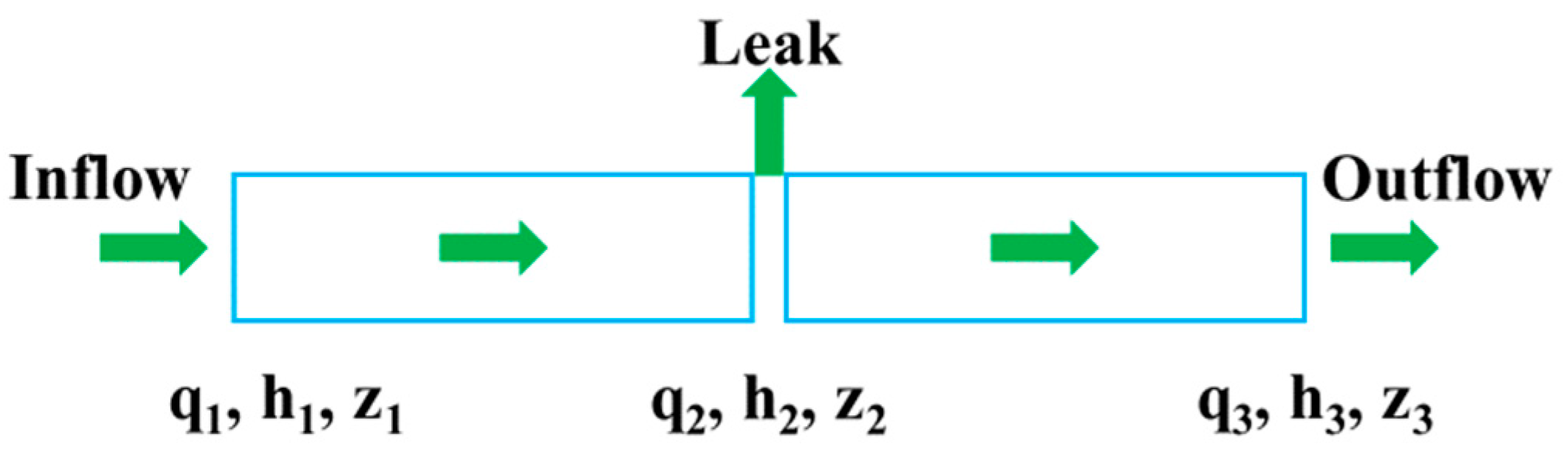
2.2. Pipeline Leakage Model
2.3. Leakage Detection Method Based on EKF
2.3.1. EKF Theory
- Prediction step:
- 2.
- Update step:
2.3.2. Application of EKF in Leak Detection
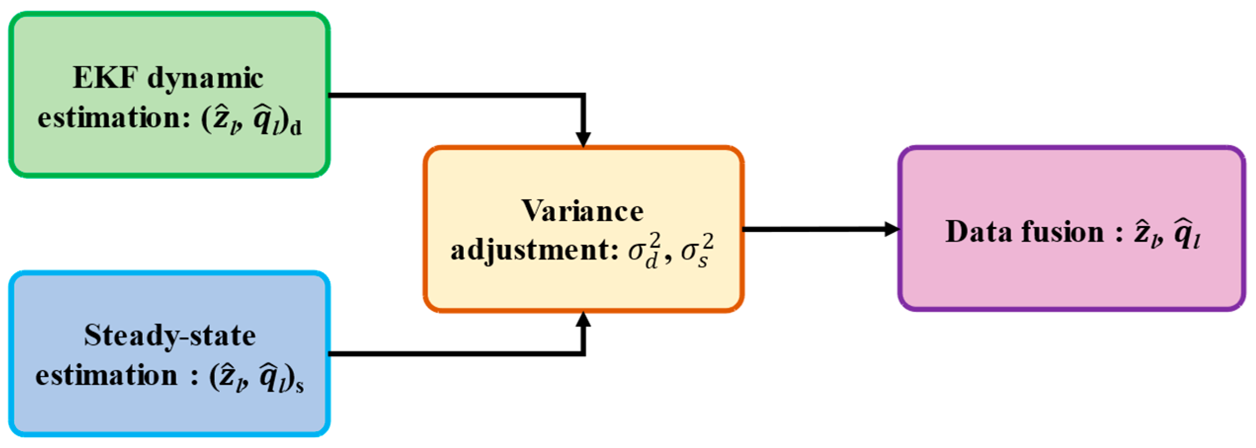
2.4. Enhancement of the EKF Algorithm with Steady-State Solution
3. Results
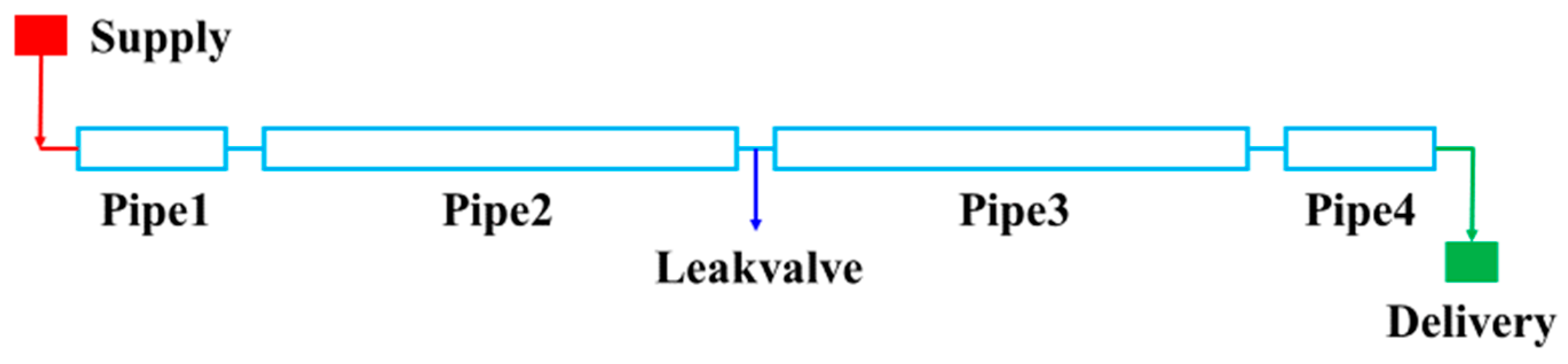
3.1. Numerical Simulation of Pipeline Leakage
3.1.1. Numerical Simulation of Pipeline Leakage Model
3.1.2. Simulation with Results of Pipeline Leakage
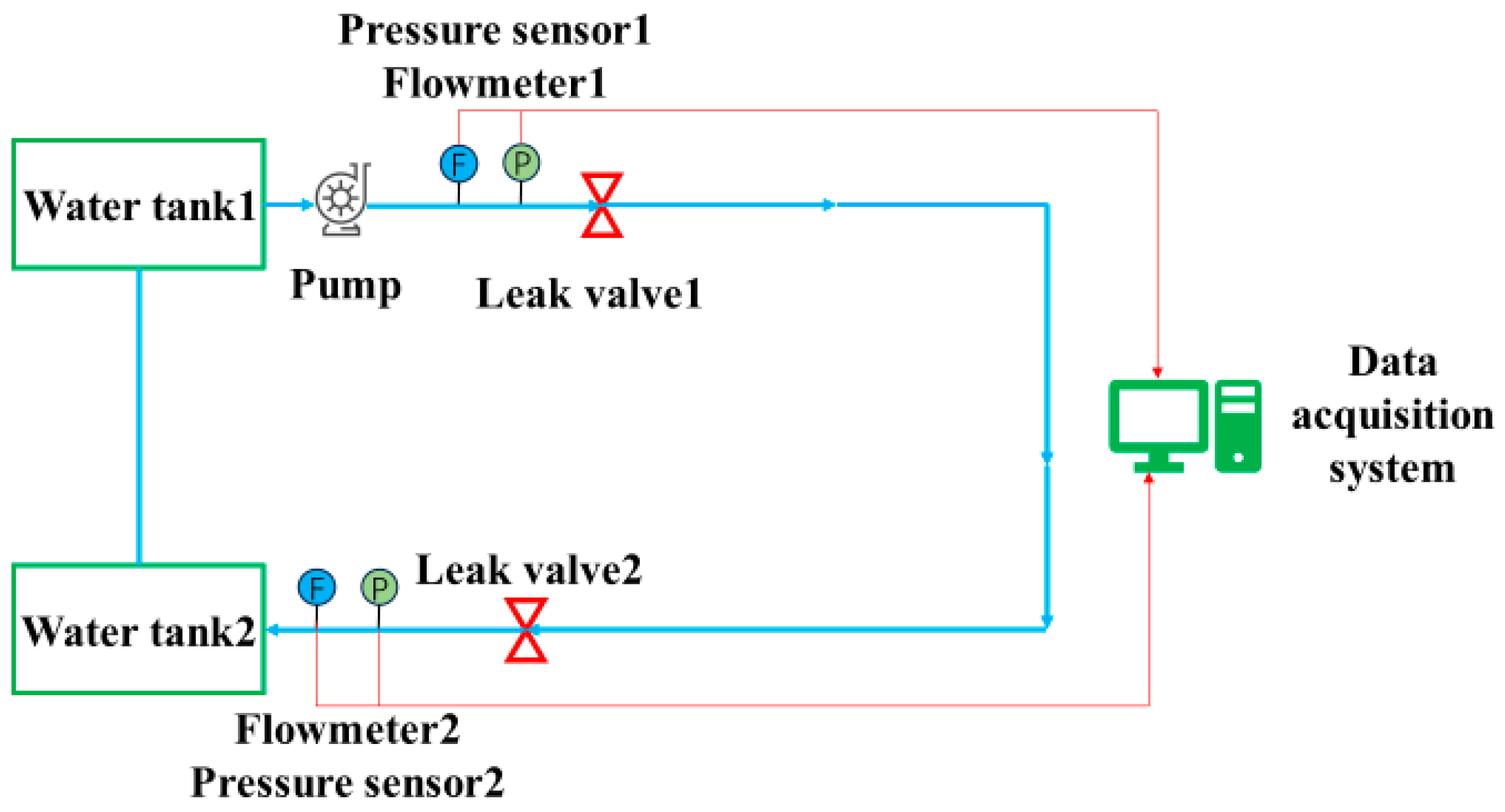
3.2. Practical Experiment and Results of Pipeline Leakage
3.2.1. Experimental Pipeline Leakage
3.2.2. Experiment and Results of Pipeline Leakage
4. Discussion
5. Conclusions
Author Contributions
Funding
Data Availability Statement
Conflicts of Interest
Abbreviations
| EKF | Extended Kalman Filter |
| LDI | Leak detection and isolation |
| KF | Kalman Filter |
| PDE | Partial Differential Equation |
References
- Ahmad, Z.; Nguyen, T.-K.; Rai, A.; Kim, J.-M. Industrial Fluid Pipeline Leak Detection and Localization Based on a Multiscale Mann-Whitney Test and Acoustic Emission Event Tracking. Mech. Syst. Signal Process. 2023, 189, 110067. [Google Scholar] [CrossRef]
- Wang, J.; Ren, L.; Jia, Z.; Jiang, T.; Wang, G. A Novel Pipeline Leak Detection and Localization Method Based on the FBG Pipe-Fixture Sensor Array and Compressed Sensing Theory. Mech. Syst. Signal Process. 2022, 169, 108669. [Google Scholar] [CrossRef]
- Zhang, L.; Jiang, H.; Zhang, J.; Chen, H.; Lu, H.; Li, J.; Hu, Z.; Xie, K. Acoustic Model for Leak Detection of Water Supply Pipeline. J. Pipeline Syst. Eng. Pract. 2024, 14, 153–168. [Google Scholar] [CrossRef]
- Sekhavati, J.; Hashemabadi, S.H.; Soroush, M. Computational Methods for Pipeline Leakage Detection and Localization: A Review and Comparative Study. J. Loss Prev. Process Ind. 2022, 77, 104771. [Google Scholar] [CrossRef]
- Behari, N.; Sheriff, M.Z.; Rahman, M.A.; Nounou, M.; Hassan, I.; Nounou, H. Chronic Leak Detection for Single and Multiphase Flow: A Critical Review on Onshore and Offshore Subsea and Arctic Conditions. J. Nat. Gas Sci. Eng. 2020, 81, 103460. [Google Scholar] [CrossRef]
- Zhang, L.; Lin, W. Trend Detection and Adaptive Removal in Pressure Signal for Pipeline Leak Monitoring. IEEE Sens. J. 2024, 23, 19815–19822. [Google Scholar] [CrossRef]
- Doshmanziari, R.; Khaloozadeh, H.; Nikoofard, A. Gas Pipeline Leakage Detection Based on Sensor Fusion under Model-Based Fault Detection Framework. J. Pet. Sci. Eng. 2020, 184, 106581. [Google Scholar] [CrossRef]
- Rahiman, W.; Wu, B.; Ding, Z. Fault Detection Using High Gain Observer: Application in Pipeline System; The University of Manchester: Manchester, UK, 2008. [Google Scholar]
- Adegboye, M.A.; Fung, W.-K.; Karnik, A. Recent Advances in Pipeline Monitoring and Oil Leakage Detection Technologies: Principles and Approaches. Sensors 2019, 19, 2548. [Google Scholar] [CrossRef] [PubMed]
- Lin, P.; Kang, X.; Huang, R. Numerical Simulation Based on a Weakly Compressible Model in the Multi-Elbow Pipe. Front. Energy Res. 2024, 10, 954632. [Google Scholar] [CrossRef]
- Henrie, M.; Carpenter, P.; Nicholas, R.E. Real-Time Transient Model–Based Leak Detection; Elsevier: Amsterdam, The Netherlands, 2016; pp. 57–89. [Google Scholar]
- Delgado-Aguiñaga, J.A.; Santos-Ruiz, I.; Besançon, G.; López-Estrada, F.R.; Puig, V. EKF-Based Observers for Multi-Leak Diagnosis in Branched Pipeline Systems. Mech. Syst. Signal Process. 2022, 178, 109198. [Google Scholar] [CrossRef]
- Uilhoorn, F.E. State-space estimation with a Bayesian filter in a coupled PDE system for transient gas flows. Appl. Math. Model. 2015, 39, 682–692. [Google Scholar] [CrossRef]
- Santos-Ruiz, I.; Bermúdez, J.R.; López-Estrada, F.R.; Puig, V.; Torres, L.; Delgado-Aguiñaga, J.A. Online Leak Diagnosis in Pipelines Using an EKF-Based and Steady-State Mixed Approach. Control Eng. Pract. 2018, 81, 55–64. [Google Scholar] [CrossRef]
- Arifin, B.M.S.; Li, Z.; Shah, S.L. Pipeline Leak Detection Using Particle Filters. IFAC-PapersOnLine 2015, 48, 76–81. [Google Scholar] [CrossRef]
- Anjana, G.R.; Kumar, K.R.S.; Kumar, M.S.M.; Amrutur, B. A Particle Filter Based Leak Detection Technique for Water Distribution gSystems. Procedia Eng. 2015, 119, 28–34. [Google Scholar] [CrossRef]
- Torres, L.; Jiménez-Cabas, J.; González, O.; Molina, L.; López-Estrada, F.-R. Kalman Filters for Leak Diagnosis in Pipelines: Brief History and Future Research. J. Mar. Sci. Eng. 2020, 8, 173. [Google Scholar] [CrossRef]
- Jahanian, M.; Ramezani, A.; Moarefianpour, A.; Shouredeli, M.A. Gas Pipeline Leakage Detection in the Presence of Parameter Uncertainty Using Robust Extended Kalman Filter. Trans. Inst. Meas. Control 2021, 43, 2044–2057. [Google Scholar] [CrossRef]
- Delgado-Aguiñaga, J.A.; Besancon, G.; Begovich, O.; Carvajal, J.E. Multi-Leak Diagnosis in Pipelines Based on Extended Kalman Filter. Control Eng. Pract. 2016, 49, 139–148. [Google Scholar] [CrossRef]
- Hou, Q.; Zhu, W. An EKF-Based Method and Experimental Study for Small Leakage Detection and Location in Natural Gas Pipelines. Appl. Sci. 2019, 9, 3193. [Google Scholar] [CrossRef]
- Delgado-Aguinaga, J.; Besancon, G.; Begovich, O. Leak isolation based on Extended Kalman Filter in a plastic pipeline under temperature variations with real-data validation. In Proceedings of the 2015 23rd Mediterranean Conference on Control and Automation (MED), Torremolinos, Spain, 16–19 June 2015; IEEE: Piscataway, NJ, USA, 2015; pp. 316–321. [Google Scholar]
- Navarro-Diaz, A.; Alejandro Delgado-Aguinaga, J.; Santos-Ruiz, I.; Puig, V. Real-Time Leak Diagnosis in Water Distribution Systems Based on a Bank of Observers and a Genetic Algorithm. Water 2022, 14, 3289. [Google Scholar] [CrossRef]


| Pipeline Parameter | Value |
|---|---|
| Pipeline diameter | 0.3 m |
| Pipeline length | 60 km |
| Pipe1 and Pipe4 length | 1 km |
| Pipe2 length | 20 km |
| Pipe3 length | 40 km |
| Leak valve diameter | 0.02 m |
| Roughness | 6.9859 × 10⁻⁵ m |
| Fluid density | 1000 m3/kg |
| Fluid viscosity | 1.2 × 10⁻⁶ m2/s |
| Acceleration due to gravity | 9.8 m/s2 |
| Wave velocity | 1000 m/s |
| EKF Parameter | Value |
|---|---|
| Estimate state | [0.1, 275, 0.1, 30,000, 0.002] |
| Error covariance matrix P | |
| Covariance matrix of process noise Q | |
| Covariance matrix of measurement noise R |
| Method | Leakage Position (m) | Leakage Pressure Head (m) | Leak Flow (m3/s) | Leak Coefficient (10−4) |
|---|---|---|---|---|
| Real value | 20,000 | 227.9 | 0.0328 | 2.379 |
| Steady-state model | 20,474.667 | 225.7 | 0.0320 | 2.321 |
| EKF algorithm | 20,238.933 | 207.7 | 0.0319 | 2.273 |
| Improved method | 20,166.667 | 228.0 | 0.0325 | 2.325 |
| Device | Specifications and Model | Manufacturer or Version |
|---|---|---|
| Centrifugal Pump | CR10-5 | GRUNDFOS, Bjerringbro, Denmark |
| Electric Regulating Valve | EV-409CUN25RPT | GRAT, Wuhan, China |
| Pressure Sensor | BP93420-IX | Hengtong Electronic Ltd., Baoji, China |
| Flow Sensor | PROMASS F | Endress+Hauser, Reinach, Switzerland |
| LAN Switch | S2326TP-EI | HUAWEI, Shenzhen, China |
| Communication Module | 6ES7 341-10H02-OAE0 | SIEMENS, Nürnberg, Germany |
| PLC Programming Software | SIMATIC Manager | V5.5 |
| SCADA System Configuration Software | SIMATIC WinCC Explorer | V7.0.3.0 |
| SCADA Server | IBM System x3400M3, Intel E5506 2.13 GHz | IBM, New York, NY, USA |
| Method | Leakage Position (m) | Leakage Pressure Head (m) | Leak Flow (m3/s) | Leak Coefficient (10−4) |
|---|---|---|---|---|
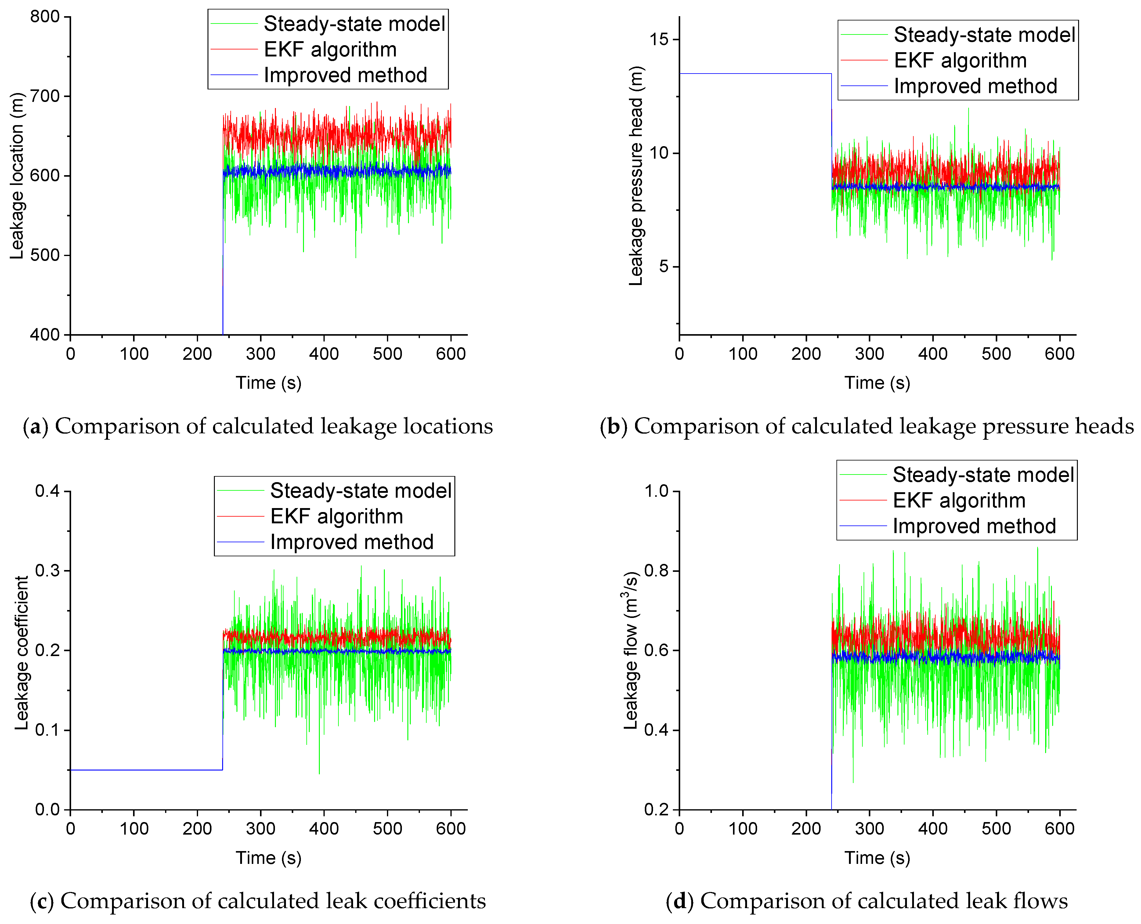
| Real value | 616.589 | 8.625 | 0.595 | 0.202 |
| Steady-state model | 650.213 | 9.184 | 0.632 | 0.216 |
| EKF algorithm | 597.692 | 8.318 | 0.568 | 0.196 |
| Improved method | 606.349 | 8.517 | 0.583 | 0.198 |
| Method | Leakage Position (m) | Leakage Pressure Head (m) | Leak Flow (m3/s) | Leak Coefficient (10−4) |
|---|---|---|---|---|
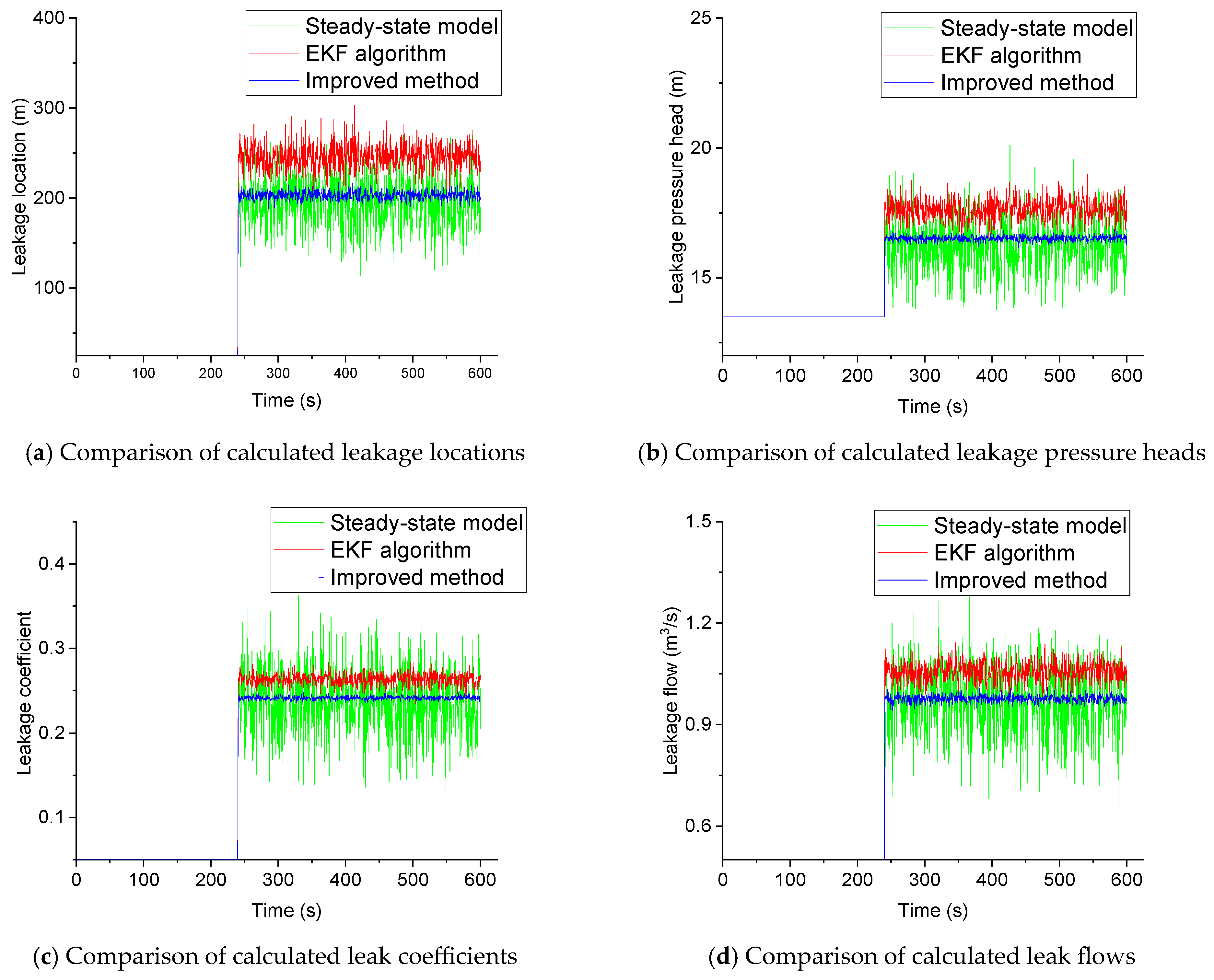
| Real value | 212.907 | 16.807 | 1.001 | 0.244 |
| Steady-state model | 246.193 | 17.656 | 1.058 | 0.263 |
| EKF algorithm | 195.652 | 16.219 | 0.962 | 0.238 |
| Improved method | 203.185 | 16.523 | 0.976 | 0.241 |
Disclaimer/Publisher’s Note: The statements, opinions and data contained in all publications are solely those of the individual author(s) and contributor(s) and not of MDPI and/or the editor(s). MDPI and/or the editor(s) disclaim responsibility for any injury to people or property resulting from any ideas, methods, instructions or products referred to in the content. |
© 2025 by the authors. Licensee MDPI, Basel, Switzerland. This article is an open access article distributed under the terms and conditions of the Creative Commons Attribution (CC BY) license (https://creativecommons.org/licenses/by/4.0/).
Share and Cite
Liu, Y.; Guo, Q.; Xie, W.; Wang, S. Enhanced Leak Detection and Localization in Liquid Pipelines Using an Improved Extended Kalman Filter. Processes 2025, 13, 1447. https://doi.org/10.3390/pr13051447
Liu Y, Guo Q, Xie W, Wang S. Enhanced Leak Detection and Localization in Liquid Pipelines Using an Improved Extended Kalman Filter. Processes. 2025; 13(5):1447. https://doi.org/10.3390/pr13051447
Chicago/Turabian StyleLiu, Yuan, Qiao Guo, Wenhao Xie, and Shouxi Wang. 2025. "Enhanced Leak Detection and Localization in Liquid Pipelines Using an Improved Extended Kalman Filter" Processes 13, no. 5: 1447. https://doi.org/10.3390/pr13051447
APA StyleLiu, Y., Guo, Q., Xie, W., & Wang, S. (2025). Enhanced Leak Detection and Localization in Liquid Pipelines Using an Improved Extended Kalman Filter. Processes, 13(5), 1447. https://doi.org/10.3390/pr13051447