Prediction of Dissolved Gas in Transformer Oil Based on Variational Mode Decomposition Integrated with Long Short-Term Memory

Abstract

To address the nonlinear and non-stationary characteristics of dissolved gas concentration data in transformer oil, this paper proposes a hybrid prediction model (VMD-SSA-LSTM-SE) that integrates Variational Mode Decomposition (VMD), the Whale Optimization Algorithm (WOA), the Sparrow Search Algorithm (SSA), Long Short-Term Memory (LSTM), and the Squeeze-and-Excitation (SE) attention mechanism. First, WOA dynamically optimizes VMD parameters (mode number k and penalty factor α to effectively separate noise and valid signals, avoiding modal aliasing). Then, SSA globally searches for optimal LSTM hyperparameters (hidden layer nodes, learning rate, etc.) to enhance feature mining for non-continuous data. The SE attention mechanism recalibrates channel-wise feature weights to capture critical time-series patterns. Experimental validation using real transformer oil data demonstrates that the model outperforms existing methods in prediction accuracy and computational efficiency. For instance, the CH₄ test set achieves a Mean Absolute Error (MAE) of 0.17996 μL/L, a Mean Absolute Percentage Error (MAPE) of 1.4423%, and an average runtime of 82.7 s, making it significantly faster than CEEMDAN-based models. These results provide robust technical support for transformer fault prediction and condition-based maintenance, highlighting the model’s effectiveness in handling non-stationary time-series data.

1. Introduction

Transformer performance plays a pivotal role in maintaining grid reliability, serving as critical infrastructure in contemporary power systems. Any operational anomaly within these devices can propagate instability across the entire network. The Dissolved Gas Analysis (DGA) technology for power transformers has currently become the most effective means for diagnosing and predicting transformer faults [1,2,3]. With the continuous development of power transformer condition estimation, fault prevention, and condition-based maintenance, the DGA technology is of great significance for predicting the dissolved gas concentration in transformer oil [4,5,6,7]. By accurately predicting the volume fraction of dissolved gases in transformer oil, the operating state of the transformer can be evaluated in advance, and operation and maintenance personnel can then be guided to formulate reasonable maintenance strategies to effectively avoid the occurrence of major accidents [8,9]. By predicting the volume fractions of dissolved gases in transformer oil and analyzing the concentrations and combinations of different gases, it is possible to identify fault types such as thermal faults, low-energy discharges, and partial discharges in advance. Therefore, research on transformer prognostics based on Dissolved Gas Analysis (DGA) is of significant importance [10,11].

However, due to the complex working environment of transformers, the collected data are usually contaminated with noise signals, making the dissolved gas concentration sequence in transformer oil highly nonlinear and non-stationary [12,13,14]. Traditional single-prediction models often struggle to cope with these complex characteristics. In order to achieve an accurate prediction of the dissolved gas concentration changes in transformer oil, scholars at home and abroad have begun to use multi-model fusion technologies.

In data denoising, noise signals are found to mainly have two characteristics: concentrated energy in the high-frequency band and a spectrum distributed in a limited interval [15,16]. Based on this, scholars have proposed many effective noise reduction methods, such as empirical mode decomposition (EMD) and Variational Mode Decomposition (VMD). EMD can decompose the original data into multiple Intrinsic Mode Functions (IMFs) according to its own characteristics, achieving adaptive decomposition. It is widely used in data denoising and has achieved remarkable results [17]. However, EMD is prone to mode mixing and end-effect problems during the decomposition process, which affects the denoising effect.

In terms of prediction methods, SVM, artificial neural networks, etc., are commonly used. For example, reference [18] proposed a prediction model for the volume fraction of dissolved gases in transformer oil based on a time series and SVM, which can achieve early-stage fault warning. However, when the data volume increases, SVM will encounter problems such as error accumulation and inability to accurately extract the temporal correlation of the data [19], limiting its application. Reference [20] used the long short-term memory neural network (LSTM) for prediction and solved some of the problems existing in SVM. However, a single LSTM model has difficulty in effectively extracting the deep-layer features of the data, restricting the further improvement of prediction accuracy. The convolutional neural network (CNN), with its own structural advantages, can layer-by-layer mine the abstract laws of data and achieve in-depth mining. However, the CNN is a static model and cannot effectively capture the long- and short-term dependencies in time series (such as the lag effects or periodic trends of gas concentration). A pure CNN may lead to error accumulation due to neglecting the correlations in the time dimension. Reference [21] combines CNN and LSTM for time series data prediction. The results show that CNN’s feature extraction can accelerate the convergence speed of the prediction model and improve prediction accuracy, but it is insufficient in modeling the interaction relationships after multimodal decomposition (e.g., high-frequency noise and low-frequency trend components decomposed by VMD). Reference [22] combines VMD with Gated Recurrent Unit (GRU) neural networks to effectively capture the temporal and nonlinear characteristics of data, improving prediction accuracy. However, it is highly sensitive to data noise and outliers, limiting the model’s generalization ability. Reference [23] weights the original volume fractions based on the attention mechanism and uses SSA to optimize the key parameters of the Bidirectional Gated Recurrent Unit (BiGRU). The constructed SSA-BiGRU-Attention model can intelligently adjust hyperparameter settings. Nevertheless, it has the problem of insufficient high-frequency noise suppression, and the attention mechanism only weights time steps, restricting the in-depth mining of multivariate coupling relationships. Reference [24] proposes a CNN-BiGRU hybrid neural network combined with Bayesian optimization. This model uses the CNN to extract high-order spatial features from multidimensional time-series data, combines the Bidirectional Gated Recurrent Unit (BiGRU) to model the long-term forward and backward dependencies of time series, employs the Bayesian optimization (BO) algorithm to dynamically search for the optimal combination of hyperparameters for CNN-BiGRU, constructs a highly correlated input feature set, and finally achieves end-to-end short-term load forecasting. However, the model has high computational complexity and strong dependence on data quality and scale.

To address the shortcomings of traditional data denoising and prediction models in terms of modal decomposition robustness, hyperparameter optimization efficiency, depth of temporal feature modeling, and multimodal interaction capabilities, the proposed VMD-SSA-LSTM-SE model achieves systematic optimization through the following four-layer progressive innovations, with specific architecture and technical breakthroughs as follows:

(1)

Dynamic VMD (Driven by WOA) to Solve Modal Aliasing and Parameter Dependence

Using the Whale Optimization Algorithm (WOA), the model dynamically searches for the optimal decomposition parameters k and α of VMD (Variational Mode Decomposition). With envelope entropy minimization as the objective function, it dynamically optimizes the parameter combination of k ∈ [4, 8] and α ∈ [800, 2500], effectively separating noise-dominated IMF (Intrinsic Mode Function) components. This achieves precise separation of noise and valid signals, avoiding modal aliasing and local information loss.

(2)

Global Hyperparameter Optimization via SSA

Leveraging the “discoverers-followers-vigilantes” mechanism of the Sparrow Search Algorithm (SSA), the model synchronously optimizes key hyperparameters of LSTM, including the number of hidden layer nodes (10–300), the learning rate (0.001–0.02), the regularization coefficient (0.0001–0.1), and training epochs (10–500). This approach features fast convergence and strong capability to escape local optima.

(3)

Construction of a Hybrid Prediction Framework: Deep Fusion of Multimodal Features and Dynamic Parameters

Through VMD denoising, feature vector reconstruction, and adaptive parameter adjustments, the framework enables the precise modeling of deep dynamic features in time-series data. Experimental results show that this framework outperforms existing methods in convergence speed, prediction accuracy, and noise robustness.

(4)

Enhancement via SE Attention Mechanism

The Squeeze-and-Excitation (SE) attention module is applied to channel-wise feature weights of LSTM outputs, dynamically recalibrating the importance of different modal components. This significantly improves the model’s ability to capture key features, especially demonstrating stronger robustness in scenarios involving trend turning points and noise interference.

2. Research Methods

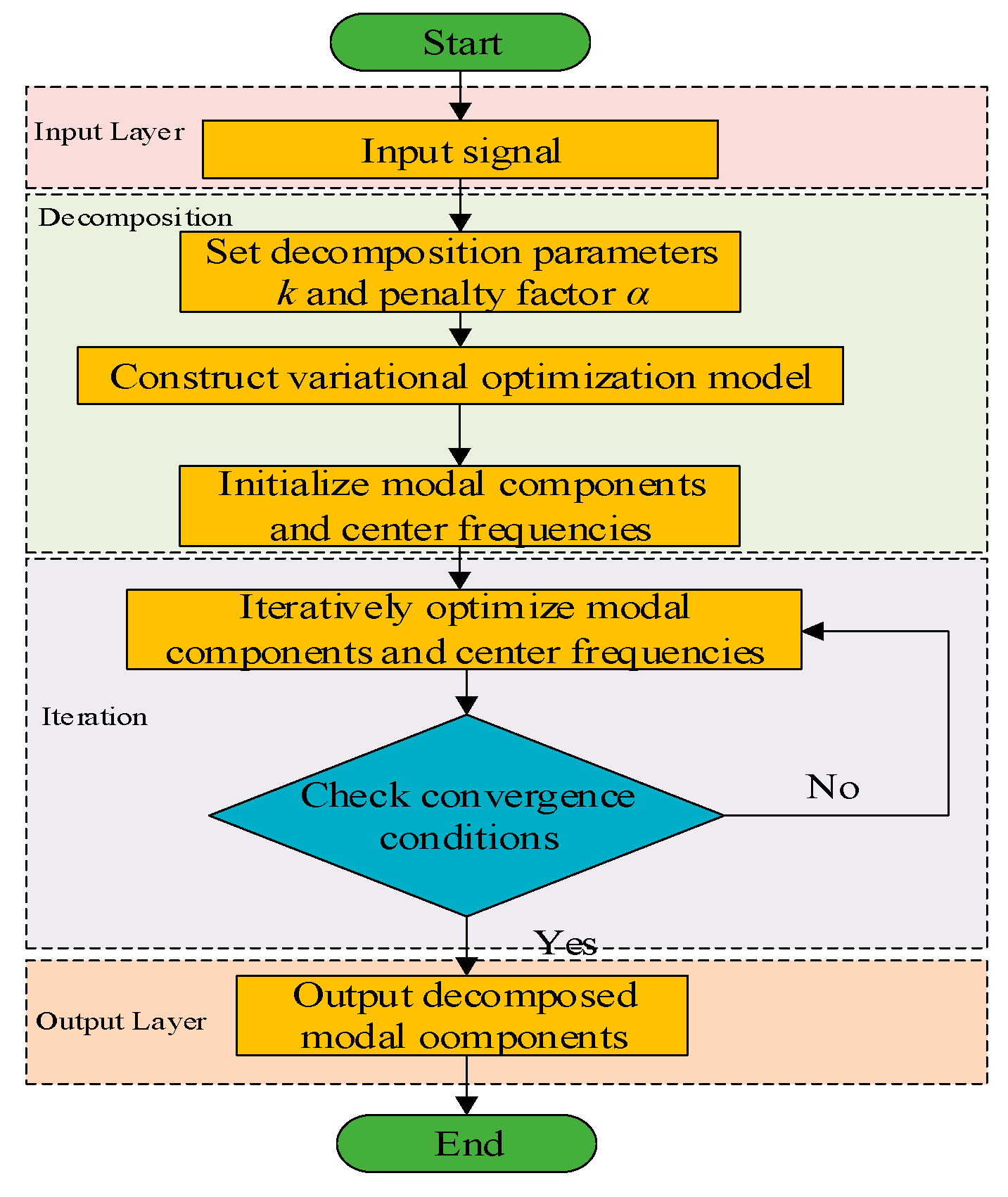
2.1. Variational Mode Decomposition

The Variational Mode Decomposition (VMD) technique decomposes the input signal f(t) into distinct modal components μ_k, each characterized by a unique central frequency ω_k. This adaptive decomposition process separates signals based on frequency localization. The input signal f(t) is decomposed into distinct modal components μ_k via Variational Mode Decomposition (VMD). The decomposition process of VMD is as follows [25,26,27]:

(1)

Construction of the variational formula

$$\mathrm{s}.\mathrm{t}.{\displaystyle \sum _{\mathrm{k}}{\mu }_k}=f(t)$$

(1)

Here, k is the number of mode functions, and f(t) is decomposed into discrete sub-signals (modes). The k-th mode μ_k is defined as

$$\underset{\left\{{\mu }_k\right\}\left\{{\omega }_k\right\}}{\min }\left\{{\displaystyle \sum _k{‖{\partial }_t[(\delta (t)+\frac{j}{\pi t}){\mu }_k(t)]{{\displaystyle e}}^{-j{\omega }_{k}t}‖}_2^2}\right\}$$

(2)

where ɷ_k is the central frequency of the k-th mode and δ(t) is the unit impulse function.

(2)

Solving the variational formula

$$\begin{array}{l}L(\left\{{\mu }_k\right\},\left\{{\omega }_k\right\},\lambda )=\alpha {\displaystyle \sum _k{‖{\partial }_t[(\delta (t)+\frac{j}{\pi t}){\mu }_k(t)]{{\displaystyle e}}^{-j{\omega }_{k}t}‖}_2^2}\\ +{‖f(t)-{\displaystyle \sum _k{\mu }_k(t)}‖}_2^2+(\lambda (t),f(t)-{\displaystyle \sum _k{\mu }_k(t)})\end{array}$$

(3)

where α is the quadratic penalty term and λ(t) is the Lagrange multiplier.

2.2. Whale Optimization Algorithm

The penalty factor α in VMD regulates the bandwidth of decomposed modes. A smaller α value increases mode overlap, whereas larger values reduce it, striking a balance between decomposition detail and computational efficiency. When the value of α is small, mode aliasing occurs, resulting in the poor decomposition of the time series. When the value of α is large, although mode aliasing can be avoided, local information loss may occur. In VMD, if the value of the mode number k is too small, under-decomposition will occur, and the hidden features in the sequence cannot be fully recognized. If the value of k is too large, over-decomposition will occur, generating false modes, which will also affect the signal decomposition effect. To effectively find the optimal parameters, this paper adaptively optimizes the parameters α and k in VMD by referring to the Whale Optimization Algorithm (WOA) in reference [28] and takes fuzzy entropy as the index of the fitness function. The smaller the fuzzy entropy value, the simpler the data sequence. The flow chart of the Whale Optimization Algorithm (WOA) is shown in Figure 1. The calculation process is as follows:

(1)

Reconstruct the N-dimensional time series {μ(j),1 ≤ j ≤ N} with dimension m:

$$\left\{\begin{array}{c}X\left(i\right)=\left[\mu \left(1\right),\mu \left(2\right),\cdots ,\mu \left(N-m+1\right)\right]-{\mu }_0\left(i\right)\\ i=1,2,\cdots ,N-m+1\\ {\mu }_0\left(i\right)={\displaystyle \frac{1}{m}}{\displaystyle \sum _{j=0}^{m-1}\mu \left(i+j\right)}\end{array}\right.$$

(4)

(2)

Calculate the distance between two m-dimensional vectors of the reconstructed time series:

$$\begin{array}{c}{d}_{ij}^m=\max \left\{\left|\mu \left(i+k\right)-{\mu }_0\left(i\right)-\mu \left(j+k\right)-{\mu }_0\left(i\right)\right|\right\}\\ i=1,2,\cdots , N-m,j=1,2,\cdots , N-m\end{array}$$

(5)

(3)

Calculate the average membership degree:

$${\phi }^m\left(n,r\right)={\displaystyle \frac{1}{N-m}}{\displaystyle \sum _{i=1}^{N-m}\left(\frac{1}{N-m-1}{\displaystyle \sum _{j=1,j\ne i}^{N-m}{D}_{ij}^m}\right)}$$

(6)

where $D_{ij}^m$ is the membership degree.

$$D_{ij}^m=\mu \left(d_{ij}^m,n,r\right)=\exp \left(-{\left(d_{ij}^m\right)}^n/r\right)$$

(7)

(4)

The fuzzy entropy function after reconstruction is given as follows:

$$\mathrm{FuzzyEn}\left(m,n,r\right)=\ln {\displaystyle \frac{{\phi }^m\left(n,r\right)}{{\phi }^{m+1}\left(n,r\right)}}$$

(8)

The fitness function of WOA is calculated using Equation (7). Optimal values of k and α are obtained when the fuzzy entropy of the VMD-decomposed sequence, computed via the above procedure, reaches its minimum.

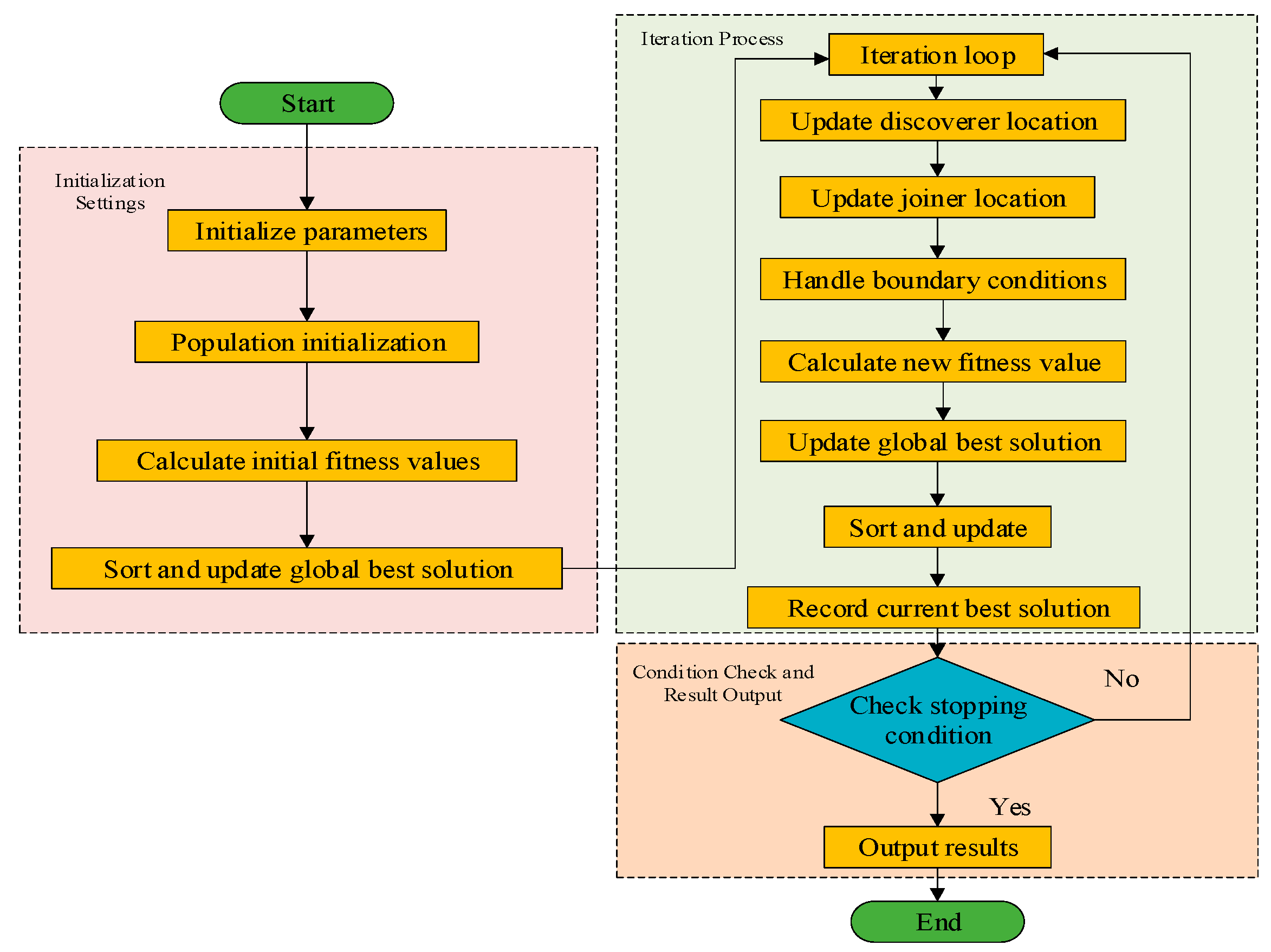
2.3. Sparrow Search Algorithm

The Sparrow Search Algorithm (SSA) can make full use of the characteristics of the algorithm such as global search ability, fast convergence, strong robustness, and adjustable parameters in transformer fault prediction [29]. The algorithm process is shown in Figure 2, and the calculation process is as follows:

(1)

The position of the discoverer is

$$x_{i,j}^{t+1}=\left\{\begin{array}{c}{x}_{i,j}^t\exp (-{\displaystyle \raisebox{1ex}{$i$}\!\left/ \!\raisebox{-1ex}{$\alpha i_{te{r}_{\max }}$}\right.}),R_2<T_s\\ x_{i,j}^t+QL,R_2\ge T_s\end{array}\right.$$

(9)

where $x_{i,j}^t$ and $x_{i,j}^{t+1}$ represent the positions of the i-th individual in the j-th dimension in the t-th and (t + 1)-th generations of the sparrow population, respectively; α ∈ (0,1] is a random number; R₂ represents the warning value; TS represents the safety value; Q is a random number, which follows a normal distribution; and L is a 1 × d dimensional matrix of 1s [30].

(2)

The position of the follower is

$$x_{i,j}^{t+1}=\left\{\begin{array}{c}Q\exp [(X_{worst}-x_{i,j}^t)i^2],R_2\le T_s\\ x_p^{t+1}+\left|x_{i,j}^t-x_p^{t+1}\right|A^{+}L\end{array}\right.$$

(10)

where x_p is the current optimal position of the discoverer; X_worst is the current global worst position; A is a 1 × d matrix, and the elements are randomly assigned 1 or −1.

(3)

The position of the vigilante is

$$x_{i,j}^{t+1}=\left\{\begin{array}{c}{X}_{best}^t+\beta \left|X_{i,j}^t-X_{best}^t\right|,f_i>f_g\\ X_{i,j}^t+K\left({\displaystyle \frac{\left|X_{i,j}^t-X_{best}^t\right|}{(f_i-f_{\omega })+\epsilon }}\right),f_i=f_g\end{array}\right.$$

(11)

β follows a normal distribution with a mean of 0 and a variance of 1; K ranges between −1 and 1; f_i represents the fitness of the current sparrow; f_g is the global optimal fitness, and f_ω is the worst; ε is a constant.

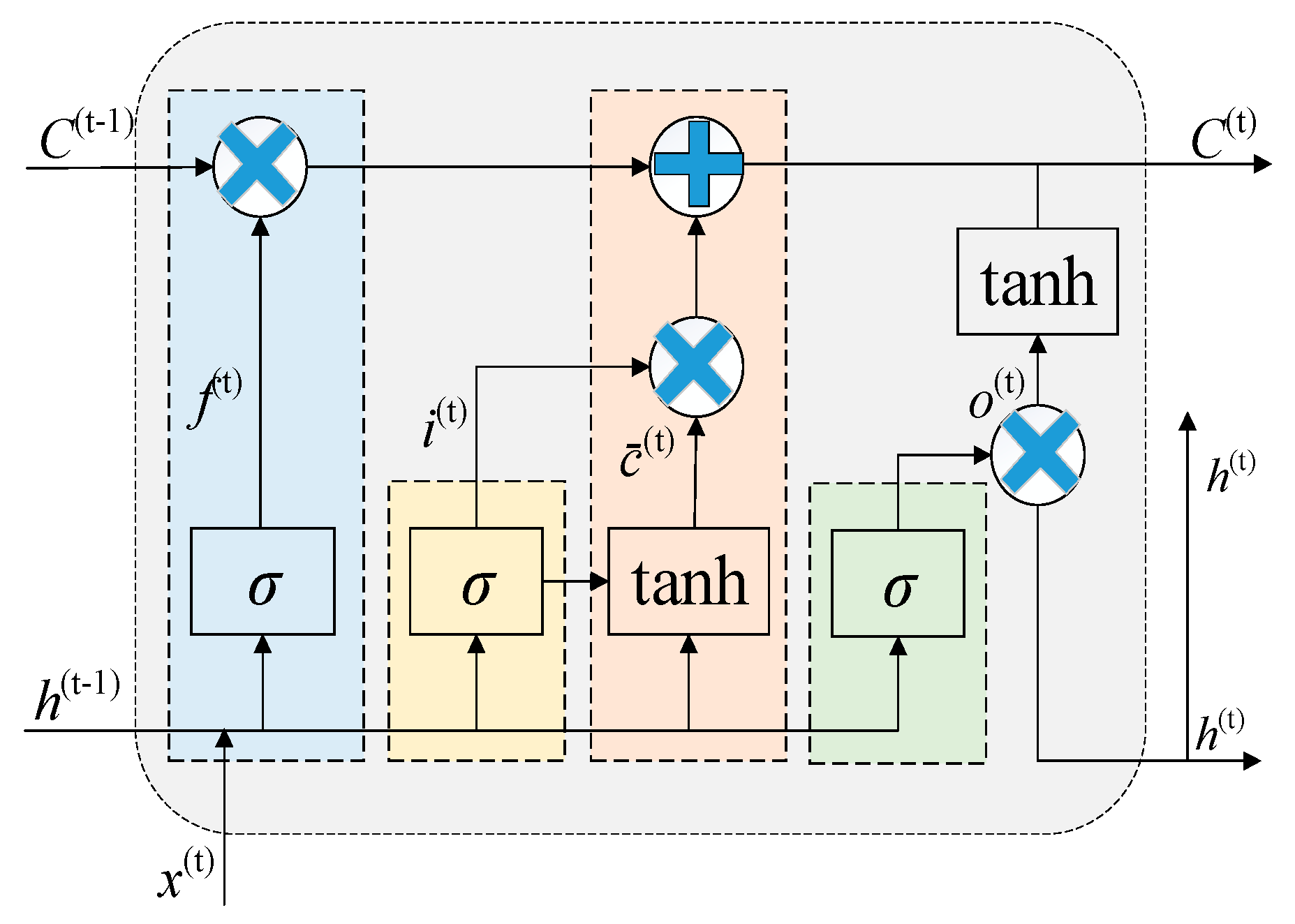
2.4. Long Short-Term Memory Neural Network

In the LSTM parameters, the max iterations, initial learning rate, optimal hidden layer nodes, and regularization coefficient most significantly impact the model’s training and fitting. Therefore, we set the search range for these four parameters in SSA and use the Root Mean Square Error (ERMSE) as the objective function for optimization.

The LSTM neural network has self-loop and gating mechanisms (forget, input, and output gates), enabling fine-grained information flow control. This structure allows LSTM to maintain stable performance in transformer fault prediction when handling long sequences. The LSTM output calculation process is shown in Figure 3 and detailed in Equations (12)–(17).

Forget gate

$$f^{(t)}=\sigma (W_f{h}^{(t-1)}+W_f{x}^{(t)}+b_f)$$

(12)

Input gate

$$i^{(t)}=\sigma (W_i{h}^{(t-1)}+W_i{x}^{(t)}+b_i)$$

(13)

Candidate cell state

$${\overline{c}}^{(t)}=\tanh (W_i{h}^{(t-1)}+W_i{x}^{(t)}+b_i)$$

(14)

Updated cell state

$$c^{(t)}=c^{(t-1)}\otimes f^{(t)}+i^{(t)}\otimes {\overline{c}}^{(t)}$$

(15)

Output gate

$$o^{(t)}=\sigma (W_o{h}^{(t-1)}+W_o{x}^{(t)}+b_o)$$

(16)

Updated hidden state

$$h^{(t)}=o^{(t)}\otimes \tanh (c^{(t)})$$

(17)

Here, i^(t) represents the input gate state of LSTM at time step t; f^(t) is the forget gate state; o^(t) is the output gate state; c denotes the memory cell, and h is the output of the hidden layer. h corresponds to the connection layer weight matrix; W represents the unit state bias term, and b is the sigmoid activation function.

2.5. Squeeze and Excitation

The SE attention mechanism, a channel attention module, learns channel correlations to recalibrate LSTM output features, enhancing multi-channel feature discrimination.

First comes the Squeeze step. The global average pooling operation can be expressed as

$$z_c={\displaystyle \frac{1}{H\times W}}{\displaystyle \sum _{i=1}^H{\displaystyle \sum _{j=1}^W{F}_{c,i,j}}}$$

(18)

where z_c is the global descriptor for channel c. For F ∈ R^C×H×W, C is the number of channels, and H and W are the height and width of the feature map.

Next is the Excitation step. The Excitation step captures channel correlations via two FC layers, reducing and reconstructing channel descriptors.

$$s=\sigma (W_2\cdot \delta (W_1\cdot z))$$

(19)

Here, W₁ ∈ R^C/r×C and W₂ ∈ R^C×C/r are weight matrices; r is the dimensionality reduction factor; δ is the ReLU activation function; σ is the Sigmoid activation function, and s represents the final channel attention weights.

Finally, element-wise multiply channel attention weights with features are used to generate attentional outputs.

$$F^{’}=s\odot F$$

(20)

where ⊙ denotes element-wise multiplication and F’ is the output feature map after applying the attention mechanism.

2.6. Construction of the VMD-SSA-LSTM-SE Prediction Model

The VMD-SSA-LSTM-SE prediction model proposed in this paper is constructed through the following steps, as shown in Figure 4:

Data Preprocessing: the concentration data of dissolved gases in transformer oil are first preprocessed, including removing obvious outliers and interpolating missing values linearly, to ensure the accuracy and consistency of the data.

VMD Decomposition: Using the Whale Optimization Algorithm (WOA) to optimize Variational Mode Decomposition (VMD), the preprocessed data are decomposed into multiple Intrinsic Mode Functions (IMFs). These IMFs have clearer physical meanings and effectively separate noise from valid signals.

LSTM Parameter Optimization: the Sparrow Search Algorithm (SSA) is employed to globally optimize key parameters of the Long Short-Term Memory (LSTM) network, such as the number of hidden layer nodes, the initial learning rate, the regularization coefficient, and the maximum training epochs, ensuring optimal parameter combinations within limited computational resources.

LSTM Model Construction: each IMF is input into the optimized LSTM model, which uses its gating mechanisms (forget gate, input gate, and output gate) to model time-series data and extract deep dynamic features.

SE Attention Mechanism Enhancement: the Squeeze-and-Excitation (SE) attention module is applied to the LSTM output features to dynamically recalibrate feature weights through channel attention, enhancing the model’s ability to capture critical features.

Model Training and Prediction: Each IMF is trained independently, and the test set data are input into these models for prediction. The final prediction results are obtained by aggregating the predictions of all IMFs.

Model Evaluation: the performance of the model is evaluated using error metrics (such as Root Mean Square Error (RMSE), Mean Absolute Error (MAE), and Mean Absolute Percentage Error (MAPE)).

3. Model Application and Experimental Validation

3.1. Data Sources and Experimental Platform Configuration

This study focuses on the concentration data of five dissolved gases in oil: H₂, CH₄, C₂H₄, C₂H₆, and C₂H₂. Based on the dissolved gas data from UK substation transformers cited in reference [31], a dataset spanning from 15 August 2013 to 10 August 2014 was selected, with samples collected every 8 h, totaling 1000 entries. The first 750 samples are used as the training set, while the final 250 samples serve as the test set to evaluate the model’s predictive accuracy and generalization capability when handling unseen data.

The algorithm simulations were conducted using MATLAB 2023b, with computer hardware configured with an Intel(R) Core(TM) i7-12700 2.10 GHz processor (Lenovo (Beijing) Co., Ltd., Beijing, China) and 16 GB RAM.

3.2. Adaptive Optimization of VMD and LSTM Parameters

To address the nonlinear and non-stationary characteristics of dissolved gas concentration data in transformer oil, the model employs the WOA and SSA for hierarchical adaptive optimization of key parameters in VMD and LSTM, ensuring synergistic improvement in modal decomposition accuracy and prediction model generalization.

3.2.1. WOA-Based VMD Parameter Optimization

The core parameters of VMD—the number of modes k and penalty factor α—directly influence signal decomposition quality. A too-small k leads to under-decomposition, failing to fully extract hidden features, while a too-large k may introduce spurious modes and exacerbate over-decomposition. The penalty factor α controls the modal bandwidth; an excessively small α causes modal aliasing, whereas an excessively large α may result in local information loss. The WOA is introduced to dynamically search for the optimal parameter combination, using fuzzy entropy minimization (Equation (8)) as the objective function within a preset range (

Table 1. Optimization interval for VMD parameters.

Parameters	Value Range
α	[800, 2500]
k	[4, 8]

).

Experiments show that the value of k within the range of [4, 8] balances the decomposition detail and computational efficiency. Within the range of [800, 2500], α is dynamically adjusted according to the spectral characteristics of different gases, effectively separating noise-dominated Intrinsic Mode Function (IMF) components (e.g., IMF1 of CH₄ captures low-frequency trends, while IMFs 2–6 correspond to high-frequency noise), providing high signal-to-noise ratio input features for subsequent LSTM modeling.

During the optimization process, WOA iteratively updates k and α in the solution space until the fuzzy entropy converges to the minimum value. For the five characteristic gases (H₂, CH₄, C₂H₂, C₂H₆, and C₂H₄), the optimized parameter combinations significantly enhance the robustness of modal decomposition, avoiding decomposition biases caused by traditional fixed parameters. The specific optimization results are shown in

Table 2. VMD parameter values after optimization via the WOA.

Parameters	H2	CH4	C2H2	C2H6	C2H4
α	2106	1926	1989	1836	2069
k	5	6	4	6	5
Optimal fitness	0.00192	0.00124	0.02583	0.00121	0.00012

.

3.2.2. SSA-Based LSTM Hyperparameter Optimization

The prediction performance of the LSTM network highly depends on hyperparameter settings. For four key parameters, namely the number of hidden layer nodes, learning rate, regularization coefficient, and training epochs, SSA is used for global optimization. SSA synchronously searches for the optimal parameter combination within a preset range (

Table 3. Optimization interval for LSTM parameters.

Parameters	Value Range
Hidden layer node count	[10, 300]
Initial learning rate	[0.001, 0.02]
Maximum training epochs	[10, 500]
Regularization coefficient	[1.0 × 10−8, 0.1]

) through a three-stage collaboration mechanism of “discoverers-followers-vigilantes”, avoiding local optima.

Using the Root Mean Square Error (RMSE) as the objective function, SSA dynamically adjusts population positions (Equations (9)–(11)) during iterations to converge rapidly to the optimal solution. Taking the CH₄ prediction as an example, the optimized number of hidden layer nodes is 84, and the learning rate is 0.00397, thus reducing the training set MAPE by 1.29% compared with unoptimized LSTM and verifying the effectiveness of parameter optimization in enhancing the model’s feature mining capability. Specific optimization results are shown in

Table 4. LSTM parameter values after optimization using the SSA.

Parameters	H2	CH4	C2H2	C2H6	C2H4
Hidden layer node count	164	84	246	277	119
Initial learning rate	0.00208	0.00397	0.01	0.00817	0.00221
Maximum training epochs	279	211	297	220	274
Regularization coefficient	0.0001	1.0 × 10−8	1.0 × 10−8	1.0 × 10−8	1.0 × 10−8

.

The parameter ranges are set to balance LSTM model complexity and overfitting risk; insufficient hidden layer nodes cause underfitting, while excessive nodes increase computational costs; a too-high learning rate may destabilize training, while a too-low rate slows convergence. SSA achieves optimal parameter combinations with limited computational resources through adaptive adjustments, laying the foundation for the deep modeling of multimodal features.

3.2.3. Synergistic Effect of Optimization Strategies

The parameter optimizations of VMD and LSTM form a complementary relationship: WOA solves the parameter dependence problem of modal decomposition to ensure input feature effectiveness, while SSA tunes the nonlinear mapping capability of LSTM to improve adaptability to non-stationary sequences. Their synergistic effect significantly reduces prediction errors in subsequent experiments (e.g., CH₄ test set MAE of 0.17996 μL/L), verifying the scientificity and necessity of the hierarchical optimization strategy.

3.3. VMD-Based Dissolved Gas Data Decomposition and Feature Separation

3.3.1. Data Preprocessing and Modal Decomposition Process

The original dissolved gas concentration sequence undergoes preprocessing to enhance data quality; obvious outliers are detected and removed using the 3σ criterion, and missing values are repaired via linear interpolation to ensure sequence integrity and continuity. Subsequently, the preprocessed data are decomposed using VMD with parameters (α and k) optimized by WOA. Taking the CH₄ prediction as an example, the optimized parameters are k = 6 and α = 1926 (with an optimal fitness of 0.00124), which avoid modal aliasing while preserving key trend features of the signal.

3.3.2. Case Study of Characteristic Gas Decomposition: CH₄ Sequence Example

As shown in Figure 5, the original CH₄ signal contains complex frequency components and noise, which are decomposed into six IMF components by VMD. IMF1, as the low-frequency principal component, captures the long-term trend of gas concentration, reflecting the core evolution pattern of transformer operating states. From IMF2 to IMF6, the frequency increases with the component number, corresponding to high-frequency noise, short-term fluctuations, and local detail information. This frequency-localized decomposition effectively separates noise from valid signals, endowing each IMF component with clear physical meanings, namely low-frequency components for trend modeling and high-frequency components for capturing abnormal fluctuations, providing multi-scale, high-signal-to-noise ratio input features for the LSTM neural network. By inputting each IMF component into the optimized SSA-LSTM-SE model independently, targeted modeling of different frequency components is achieved, significantly improving the model’s feature parsing ability for non-stationary time-series data.

3.4. Model Prediction Experiments and Performance Evaluation

3.4.1. Evaluation Metrics and Comparative Methods

Three core metrics—Root Mean Square Error (RMSE), Mean Absolute Error (MAE), and Mean Absolute Percentage Error (MAPE)—are employed to comprehensively evaluate the model from absolute error, typical error magnitude, and relative error perspectives. RMSE is sensitive to outliers, so it is suitable for quantifying the overall error scale; MAE measures prediction bias via linear distance, offering robustness against noise; MAPE presents relative errors as percentages, facilitating accuracy comparison across datasets of different scales. The formulas are as follows:

$$E_{RMSE}=\sqrt{{\displaystyle \frac{1}{n}}{\displaystyle \sum _{i=1}^n{(y_i-{\widehat{y}}_i)}^2}}$$

(21)

$$E_{MAE}={\displaystyle \frac{1}{n}}{\displaystyle \sum _{i=1}^n\left|y_i-{\widehat{y}}_i\right|}$$

(22)

$$E_{MAPE}={\displaystyle \frac{1}{n}}{\displaystyle \sum _{i=1}^n\left|\frac{y_i-{\widehat{y}}_i}{y_i}\right|}\times 100\%$$

(23)

In the formulas, n is the number of prediction samples; y_i is the predicted concentration of the dissolved gas in oil at time i, and ${\widehat{y}}_i$ is the actual concentration of the dissolved gas in oil at time i.

3.4.2. Multi-Model Comparative Experiments and Result Analysis

To validate the effectiveness of the proposed model, VMD-SSA-LSTM-SE is compared with five baseline models (VMD-LSTM, VMD-LSTM-SE, CNN-LSTM, VMD-SSA-LSTM, and CEEMDAN-VMD-SSA-LSTM-SE). The proposed model employs adaptive parameter selection, while the parameters of LSTM, SSA, and VMD for the remaining models are listed in

Table 5. Configuration of the training and testing parameters for model validation.

Parameter Category	Parameter Name	Description/Value
LSTM hyperparameters	LSTM neurons	30
	Fixed training epochs	30
	Fixed learning rate	0.001
	Fixed regularization coefficient	0.0001
SSA parameters	SSA population size	3
	SSA maximum iterations	4
VMD parameters	k	5
	α	2000

.

As shown in Figure 6, SSA converges to optimal parameters within limited iterations, verifying its efficient optimization capability under resource constraints. Taking the CH₄ sequence as an example (Figure 7), the proposed model’s prediction curve closely aligns with actual values, demonstrating strong tracking at trend turning points. The test set’s fluctuations are significantly lower than those of comparative models, highlighting excellent generalization to non-stationary data. Error comparisons (Figure 8) show that VMD-SSA-LSTM-SE and CEEMDAN-VMD-SSA-LSTM-SE have the steadiest error curves, but the former runs 34.7% faster (82.7 s vs. 126.6 s for CH₄), balancing precision and efficiency.

3.4.3. Generalization Ability and Computational Efficiency Verification

Table 6. Comparison of training set errors among three prediction models.

Model	Evaluation Parameters	Gas Concentration in Transformer Oil
		H2	CH4	C2H2	C2H6	C2H4
VMD-LSTM	ERMSE/(μL/L)	0.52954	0.22219	0.05743	0.48661	0.15879
	EMAE/(μL/L)	0.39095	0.17250	0.04378	0.38129	0.12329
	EMAPE %	4.9169%	2.8638%	3.0483%	7.7377%	9.9218%
VMD-LSTM-SE	ERMSE/(μL/L)	0.40484	0.19835	0.07681	0.41791	0.11992
	EMAE/(μL/L)	0.25912	0.14929	0.05782	0.32185	0.08774
	EMAPE %	3.6045%	2.4637%	3.9975%	6.4496%	7.0205%
CNN-LSTM	ERMSE/(μL/L)	0.42631	0.40811	0.12903	0.78602	0.16579
	EMAE/(μL/L)	0.22801	0.30544	0.09991	0.62561	0.12724
	EMAPE %	1.2597%	3.5401%	6.8256%	7.4477%	5.7834%
VMD-SSA-LSTM	ERMSE/(μL/L)	0.11232	0.04330	0.01116	0.07104	0.01959
	EMAE/(μL/L)	0.06384	0.03410	0.00849	0.05656	0.01548
	EMAPE %	0.88436%	0.56203%	0.59143%	1.1283%	1.2963%
CEEMDAN-VMD-SSA-LSTM-SE	ERMSE/(μL/L)	0.14023	0.06239	0.02492	0.10581	0.02438
	EMAE/(μL/L)	0.09689	0.04977	0.01908	0.08292	0.01978
	EMAPE %	1.1802%	0.82958%	1.3155%	1.6352%	1.6275%
VMD-SSA-LSTM-SE	ERMSE/(μL/L)	0.10027	0.04395	0.01206	0.07014	0.02255
	EMAE/(μL/L)	0.05698	0.03475	0.00943	0.05562	0.01770
	EMAPE %	0.7573%	0.57308%	0.65146%	1.114%	1.4696%

and

Table 7. Comparison of test set errors among three prediction models.

Model	Evaluation Parameters	Gas Concentration in Transformer Oil
		H2	CH4	C2H2	C2H6	C2H4
VMD-LSTM	ERMSE/(μL/L)	0.72277	0.43937	0.09040	0.71347	0.21429
	EMAE/(μL/L)	0.64305	0.34941	0.07035	0.61983	0.18705
	EMAPE %	5.9566%	4.2223%	3.6863%	7.3852%	12.323%
VMD-LSTM-SE	ERMSE/(μL/L)	0.39484	0.48268	0.10079	0.47545	0.14626
	EMAE/(μL/L)	0.24912	0.40457	0.08397	0.38084	0.11724
	EMAPE %	3.2045%	4.8871%	4.1376%	4.8962%	7.7415%
CNN-LSTM	ERMSE/(μL/L)	1.06310	1.17661	0.21547	0.85926	0.18664
	EMAE/(μL/L)	0.84994	1.04832	0.16818	0.68918	0.15119
	EMAPE %	8.3209%	12.6144%	9.1034%	9.085%	10.1605%
VMD-SSA-LSTM	ERMSE/(μL/L)	0.63073	0.21866	0.06736	0.5198	0.03086
	EMAE/(μL/L)	0.33350	0.17521	0.04641	0.41104	0.02482
	EMAPE %	2.2521%	2.13%	2.592%	5.6151%	1.7637%
CEEMDAN-VMD-SSA- LSTM-SE	ERMSE/(μL/L)	0.73033	0.86777	0.18498	0.72829	0.13782
	EMAE/(μL/L)	0.31158	0.28236	0.06772	0.32207	0.03983
	EMAPE %	2.1528%	2.0902%	2.3323%	3.1726%	1.5399%
VMD-SSA-LSTM-SE	ERMSE/(μL/L)	0.63047	0.48942	0.18664	0.67918	0.09714
	EMAE/(μL/L)	0.21031	0.17996	0.086103	0.31882	0.04332
	EMAPE %	1.2648%	1.4423%	2.6433%	2.892%	2.2952%

show that VMD-SSA-LSTM-SE achieves a training set MAPE of 0.5731%, an RMSE of 0.04395 μL/L, and an MAE of 0.03475 μL/L for CH₄, outperforming all baseline models. The test set’s MAPE is 1.4423% and 0.17996 μL/L for MAE, confirming stable performance across datasets. For other gases (H₂, C₂H₂, etc.), the model maintains the lowest or near-lowest errors in both training and test sets, demonstrating universality for multi-characteristic gases.

In terms of computational efficiency (

Table 8. Runtime of six models (seconds).

Model	H2	CH4	C2H2	C2H6	C2H4
VMD-LSTM	6.6	7.7	2.2	3.4	3.2
VMD-LSTM-SE	2.22	3.28	2.3	2.2	2.22
CNN-LSTM	5.40	4.78	6.3	6.5	5.4
VMD-SSA-LSTM	165.9	104.7	116.5	145.3	148.9
CEEMDAN-VMD-SSA-LSTM-SE	189.1	126.6	83.6	284.1	182.1
VMD-SSA-LSTM-SE	63.5	82.7	44.7	98	56.7

), the model averages a runtime of 71.1 s, which is over 50% faster than CEEMDAN-VMD-SSA-LSTM-SE (169.1 s) and significantly better than VMD-SSA-LSTM (136.3 s). This efficiency stems from hierarchical optimization by WOA-SSA, reducing invalid parameter searches, and VMD’s effective noise separation, lowering training complexity. Combining error metrics and runtime, VMD-SSA-LSTM-SE stands out as the optimal solution for real-time prediction of dissolved gas concentrations in transformers.

4. Discussion

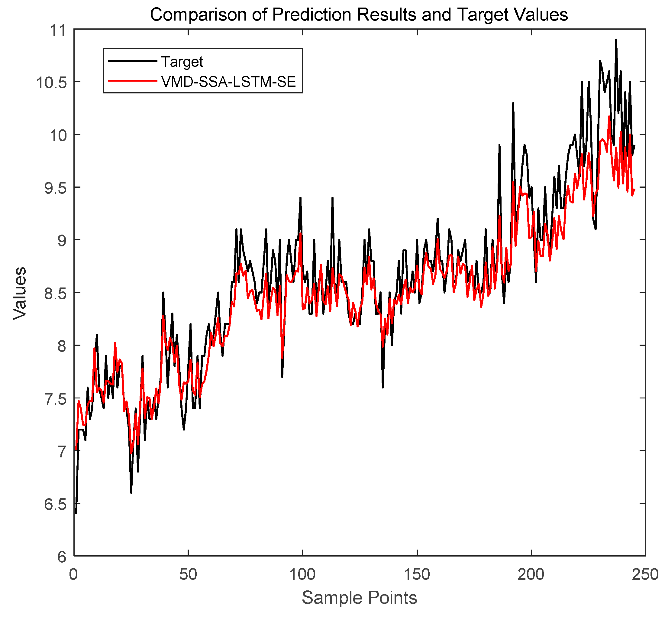
The VMD-SSA-LSTM-SE model has the lowest ERMSE values for H₂, CH₄, C₂H₂, C₂H₆, and C₂H₄, indicating the highest prediction accuracy for these gases. The CEEMDAN-VMD-SSA-LSTM-SE model has a slightly lower ERMSE for C₂H₂ but underperforms in other gases compared to the VMD-SSA-LSTM-SE model. The VMD-SSA-LSTM-SE model also has the lowest EMAE values for all gases, further confirming its high prediction accuracy. While the CEEMDAN-VMD-SSA-LSTM-SE model has slightly higher EMAE values for some gases, its overall performance is still relatively close.

In terms of EMAPE, the VMD-SSA-LSTM-SE model again has the lowest values for all gases, indicating the smallest proportion of prediction error relative to the actual values. The CEEMDAN-VMD-SSA-LSTM-SE model has slightly higher EMAPE values for some gases but remains relatively close in overall performance. With an average runtime of 71.1 s, the VMD-SSA-LSTM-SE model is not the fastest, but its runtime is significantly shorter than that of the CEEMDAN-VMD-SSA-LSTM-SE model (169.1 s) and the VMD-SSA-LSTM model (136.3 s) while still maintaining high precision.

In summary, considering both prediction performance across all gases and runtime, the VMD-SSA-LSTM-SE model outperforms the others in terms of evaluation metrics (ERMSE, EMAE, and EMAPE) and has a significant advantage in runtime.

5. Conclusions

This study proposes a hybrid prediction model (VMD-SSA-LSTM-SE) that integrates VMD, WOA, SSA, LSTM, and the SE attention mechanism for high-precision forecasting of dissolved gas concentrations in transformer oil. Theoretical analysis and experimental validation lead to the following core conclusions:

5.1. Effectiveness of Adaptive Parameter Optimization

• By minimizing fuzzy entropy, WOA dynamically optimizes VMD parameters k and α, addressing modal aliasing and parameter dependence in traditional VMD to achieve precise separation of noise and valid signals. For example, CH₄ decomposition yields IMF1 for low-frequency trends and IMFs 2–6 for high-frequency noise, providing high-signal-to-noise input features for LSTM.
• Leveraging the “discoverers-followers-vigilantes” mechanism, SSA globally searches for optimal LSTM hyperparameters (hidden layer nodes, learning rate, regularization coefficient, and training epochs), significantly enhancing feature mining for non-continuous data with limited computational resources. The CH₄ training set MAPE decreases by 1.29% compared to unoptimized LSTM, verifying the suppression of overfitting and improved adaptability.

5.2. Critical Role of Attention Mechanism,

The SE module dynamically recalibrates channel-wise feature weights, enhancing the expression of key modal components and improving robustness in trend turning points and noisy environments. Experiments show that the average test set MAPE for five characteristic gases is 2.11%, which is a 1.32% reduction compared to models without SE, effectively improving the discriminative ability for multimodal features

5.3. Dual Advantages in Prediction Accuracy and Computational Efficiency

• The model achieves an MAE of 0.17996 μL/L and an MAPE of 1.4423% for CH₄ in the test set, outperforming comparative models like VMD-LSTM and CNN-LSTM. For other gases (H₂, C₂H₂, etc.), it consistently shows the lowest or near-lowest RMSE, MAE, and MAPE in both training and test sets, demonstrating universality for different gas concentration sequences.
• With an average runtime of 71.1 s, the model is over 50% faster than CEEMDAN-VMD-SSA-LSTM-SE (169.1 s), balancing high accuracy with real-time requirements for engineering applications.

5.4. Engineering Application Value

This model provides a reliable tool for transformer fault early warning, assisting maintenance personnel in formulating precise inspection strategies by predicting dissolved gas concentration changes in advance, thereby reducing grid failure risks. Its hierarchical optimization architecture and multi-technology fusion approach offer a methodological reference for predicting other nonlinear and non-stationary time-series data. In summary, this model offers a reliable tool for transformer fault early warning. By predicting dissolved gas concentration changes in advance, it aids maintenance personnel in devising precise inspection strategies, reducing the risk of power grid failures.