Machine Learning-Based Impact of Rotational Speed on Mixing, Mass Transfer, and Flow Parameter Prediction in Solid–Liquid Stirred Tanks

Abstract

To address the issues of low solid–liquid mixing and mass transfer efficiency and difficult real-time regulation in the resource utilization of non-ferrous metal smelting slag, this study constructs a research framework integrating Computational Fluid Dynamics-Discrete Element Method (CFD-DEM) coupling models and machine learning. The framework systematically investigates particle motion characteristics and mass transfer laws in stirred tanks and enables an intelligent prediction of key parameters. Through a CFD-DEM two-way coupling simulation, the study quantifies particle dispersion characteristics using relative standard deviation (RSD) and calculates the mass transfer coefficient (k) based on the Hughmark model, revealing the effects of particle size and impeller speed on mixing and mass transfer efficiency. For parameter prediction, particle motion and mass transfer data are used to train a multi-model prediction library, with model performance evaluated through comparative experiments. The results show that increasing the rotational speed shortens the particle mixing time, reduces RSD values by 25–40%, increases the coupling force, and decreases stability during the circulation phase. Different machine learning (ML) algorithms exhibit varying performances in the time-series prediction of particle motion characteristics and real-time prediction of mass transfer coefficients. Notably, GA-BP achieves a fitting degree R of 0.99 in both predictions, meeting the requirements for the structural optimization and intelligent regulation of stirred tanks. This research provides theoretical support and technical pathways for the structural optimization and intelligent control of stirred tanks, offering engineering application value in fields such as hydrometallurgy and solid waste resource utilization.

1. Introduction

As critical national strategic resources, Vanadium and its compounds are widely applied in steel, chemical, electronics, and energy sectors. Achieving clean and efficient vanadium extraction from mineral resources and recycling vanadium from smelting slag aligns with the national strategic needs for high-quality development [1]. In solid–liquid mixing during the resource utilization of non-ferrous metal smelting slag, challenges include balancing leaching efficiency with economic and operational feasibility, the synergy between mass transfer and chemical reactions, the effects of particle size and agitation speed, and the adaptation of kinetic models to industrial processes. To address these issues, Gharabaghi et al. [2] optimized process parameters using statistical experimental design combined with response surface methodology (RSM), achieving 99.57% metal recovery while reducing environmental risks. Karacahan et al. [3] integrated statistical experimental design, kinetic modeling, and environmentally friendly processes to develop mathematical models describing reaction kinetics and experimental parameters, enabling efficient and sustainable metal recycling.

Solid–liquid suspension is a two-phase mixing process in which rotating agitators disperse solid particles uniformly in liquid [4]. Its core feature is overcoming particle pull-down trends through agitation to achieve efficient mass transfer at the solid–liquid interface [5]. Key influencing factors include agitator-system parameters (impeller type, rotational speed, tank geometry), solid-phase properties (particle size, density), and liquid-phase characteristics (viscosity, rheological behavior) [6]. Research methodologies integrate experimental and numerical approaches: advanced techniques like particle image velocimetry (PIV) and laser Doppler velocimetry (LDV) capture flow field details and particle trajectories [7], while CFD-DEM coupling provides microscale insights into particle agglomeration, collisions, and kinetic behaviors to support industrial scaling. Widely applied in chemical and pharmaceutical sectors, this technology optimizes mixing efficiency and mitigates engineering risks. Stirred tanks, as the core equipment in hydrometallurgical vanadium extraction, enhance mass transfer between mineral particles and solvents via impeller shear forces while precisely controlling reaction conditions (temperature, pressure, velocity). Their mixing efficiency directly impacts heat and mass transfer performance in solid–liquid systems, with critical applications in heterogeneous catalysis, biohydrogen production, and flotation separation [8]. While optimizing stirred tank mixing efficiency remains a research hotspot, technical bottlenecks persist in understanding multiphase flow turbulence characteristics and dynamic flow field regulation mechanisms. Integrating numerical simulation methods to analyze complex flow behaviors is essential for achieving efficient, low-carbon solid waste resource utilization [9].

Regarding optimizing mixing efficiency in stirred tanks, Gu et al. [10] compared self-similar impellers with RT impellers using the detached eddy simulation (DES) method. They found that, under the condition of equal power, self-similar impellers can improve the liquid–liquid equilibrium and mean-square error performance. The mixing time is shortened, and the efficiency increases with the number of iterations. Hu et al. [11] found that, when dealing with materials with large particle sizes and high solid–liquid ratios, the circular-bottom tank exerts significantly better solid-phase suspension effects than the flat-bottom tank, effectively suppressing pull-down. Ashraf et al. [12] confirmed through cloud height measurement that the baffle design can improve the uniformity of concentration distribution, revealing the positive effect of baffles on suppressing pull-down. Li et al. [13] analyzed particle motion trajectories, vortices, and collisions using the CFD-DEM two-way coupling method and constructed a particle motion model. Luo et al. [14] applied it to solid–liquid convective heat transfer. They found that reducing the blade height and increasing the baffles can optimize the stirred tank’s heat transfer efficiency and particle mixing effect. Ultimately, it is shown that the CFD-DEM coupling method is effective and reliable in solving problems related to multiphase flow particle motion and heat transfer.

Due to the inherently strong nonlinearity of stirred tanks, traditional methods cannot achieve the real-time prediction of factory data. With the rapid advancements in artificial intelligence and computer science, the integration of CFD and ML technologies has emerged as a powerful tool for real-time prediction in stirred tanks. This interdisciplinary approach demonstrates significant advantages and broad application prospects in handling multi-parameter optimization, nonlinear relationship fitting, prediction accuracy improvement, regression analysis, and operational cost reduction. As effective tools, artificial neural networks (ANNs) have been widely applied in the modeling, optimization, computation, and prediction of complex systems [15,16,17,18]. Wu et al. [15] developed an ANN-CFD turbulence state prediction model, investigating model hyperparameters using three training and optimization algorithms. By validating free surface and fluid velocities at different rotational speeds and aiding optimization with a double-layer genetic algorithm, they achieved regression metrics exceeding 0.9 for the optimized ANN-CFD model, demonstrating its excellent performance in predicting flow field states. Zhao et al. [19] employed an efficient optimization framework combining CFD, ML, and multi-objective genetic algorithms to optimize stirred tank performance. Through a single-factor analysis and the comparison of prediction parameters across different ML algorithms, they identified optimal design parameters via the Pareto front, achieving 12.3% energy consumption reduction and 13.4% mixing time reduction. This further validated the accuracy and reliability of ML-based stirred tank optimization methods. Cheng et al. [20] analyzed a pressure-fluctuation time series in fluidized beds using multiple ML algorithms, designing single-step and multi-step future state prediction tasks as regression problems. The results showed that BP performed best in single-step prediction (R² close to 1.0), while LSTM excelled in multi-step prediction, accurately forecasting fluctuations up to 34 subsequent time points. This confirmed the feasibility of ML methods for nonlinear time series analysis.

With the extensive application of high-performance computing (HPC) in fields such as large-scale scientific computing, engineering simulation, data analysis, and artificial intelligence (AI), HPC application software is facing multiple challenges, including complex functionality, short iteration cycles, and cross-platform compatibility. Traditional development models often employ offline compilation, manual testing, and manual deployment, which struggle to meet the requirements for efficiency, stability, and automation in HPC environments. Therefore, constructing a rapid development platform for HPC application software that enables full lifecycle management and automated operations and maintenance has become a critical issue requiring urgent resolution. The rapid development platform proposed in this paper aims to integrate tools such as online IDE, code hosting, automated testing, automated building, and continuous integration/continuous deployment (CI/CD) to construct an efficient, collaborative, and automated development environment.

In the field of solid–liquid stirred tank prediction, computer vision technologies (such as PIV) can experimentally validate CFD-DEM simulation results to enhance model accuracy. Meanwhile, two advanced vision models—DeepLab and EfficientNet—can broaden and deepen the research. DeepLab, based on the convolutional neural network (CNN) architecture, utilizes dilated convolutions to capture multi-scale contextual information without compromising resolution, enabling precise semantic image segmentation [21]. EfficientNet, rooted in Neural Architecture Search (NAS) technology, achieves significant computational efficiency improvements while maintaining accuracy through the joint scaling of network depth, width, and resolution [22]. Both models play a crucial role in processing relevant image data, analyzing particle motion, and characterizing flow field features.

To address challenges in synergy between mass transfer and chemical reactions, effects of agitation parameters, and adaptation of models to industrial processes during solid–liquid mixing in non-ferrous metal smelting slag resource utilization, this study establishes a research framework integrating CFD-DEM coupling models and ML. The framework systematically analyzes complex flow mechanisms in multi-metal mixing processes, investigates multiscale multiphase flow and transport characteristics in non-ferrous smelting slag mixing, and overcomes the limitations of traditional methods to resolve strong nonlinearity in multiphase stirred tanks. It enables rapid responses to dynamic operating conditions and improves real-time prediction capabilities. By bridging mechanistic understanding and intelligent control through ML, this approach provides critical technical support for multiphase flow systems’ efficient and green development.

2. Materials and Methods

This study constructs a bidirectional CFD-DEM coupling numerical model and performs grid independence verification. RSD is introduced to quantify particle dispersion uniformity, analyzing the effects of particle size and rotational speed on particle motion trajectories, coupled forces, and flow field uniformity. k is calculated to investigate the impact of rotational speed on mass transfer efficiency. A dataset of 1700 multiphase flow samples is generated through CFD-DEM simulations, which are used to compare the performance of BP (backpropagation), GA-BP (genetic algorithm–backpropagation), XGBoost (extreme gradient boosting), LSTM (long short-term memory), a CNN (convolutional neural network), PINNs (physics-informed neural networks), and other algorithms in the time-series prediction of particle velocities and mass transfer coefficients. Multiple metrics are employed to evaluate model accuracy and stability, while computational costs and an accuracy analysis are integrated to address industrial applicability challenges.

2.1. Numerical Model

2.1.1. Governing Equations

To establish a micro-mechanical model of particle motion, within the DEM framework, all particles in the computational domain are tracked using Lagrangian methods, with translational and rotational motions governed by explicitly solving Euler’s first and second laws:

$$m_p{\displaystyle \frac{d{\mathrm{v}}_p}{dt}}={\mathrm{F}}_c+{\mathrm{F}}_{f\to p}+m_p\mathrm{g}$$

(1)

$${\mathrm{J}}_p{\displaystyle \frac{d{\omega }_p}{dt}}={\mathrm{M}}_c+{\mathrm{M}}_{f\to p}$$

(2)

where $m_p$ is the particle mass, $\mathrm{g}$ is the gravitational acceleration vector, ${\mathrm{F}}_c$ represents contact forces between particles and walls, ${\omega }_p$ is the angular velocity vector, ${\mathrm{J}}_p$ is the moment of inertia tensor, and ${\mathrm{M}}_c$ is the net torque generated by tangential forces causing particle rotation. ${\mathrm{F}}_{f\to p}$ is the additional force from fluid-phase interactions, and ${\mathrm{M}}_{f\to p}$ is the additional torque induced by fluid-phase velocity gradients.

In the CFD, the fluid phase is treated as a continuous phase, typically described by the volume-averaged classical Navier–Stokes equations. The average mass conservation equation is as follows:

$${\displaystyle \frac{\partial }{\partial t}}({\alpha }_f{\rho }_f)+\nabla ·({\alpha }_f{\rho }_f\mathrm{u})=0$$

(3)

To analyze the force mechanism of particles in the flow field, this study adopts the Haider–Levenspiel model as the drag coefficient model for spherical particles, which is defined as follows:

$$C_D={\displaystyle \frac{24}{{\mathrm{Re}}_p}}(1+A{\mathrm{Re}}_p^B)+{\displaystyle \frac{C}{1+\frac{D}{{\mathrm{Re}}_p}}}$$

(4)

The values of the correlation coefficients for spherical particles are as follows:

$$\begin{array}{c}A=0.1806\\ B=0.6459\\ C=0.4251\\ D=6880.95\end{array}$$

(5)

The Saffman lift force model is adopted to calculate the lift force. Under the condition of one-dimensional configuration, the expression for the lift force can be written as follows:

$$F_L=6.46{\rho }_f{\nu }_f^{{\displaystyle \frac{1}{2}}}{\displaystyle \frac{d_p^2}{4}}(u_x-v_x){\displaystyle \frac{d{u}_x}{dy}}{\left|{\displaystyle \frac{d{u}_x}{dy}}\right|}^{-{\displaystyle \frac{1}{2}}}$$

(6)

This expression can be generalized to three-dimensional flows as follows:

$${\mathrm{F}}_L=6.46{({\rho }_f{\mu }_f)}^{{\displaystyle \frac{1}{2}}}{\displaystyle \frac{d_p^2}{4}}{\mathrm{u}}_r\times (𝛻\times \mathrm{u}){|𝛻\times \mathrm{u}|}^{-{\displaystyle \frac{1}{2}}}$$

(7)

2.1.2. CFD-DEM Coupling

Particle motion in stirred suspensions is a critical issue in industries such as chemical engineering and mineral processing, with behavior significantly influenced by operating conditions and particle properties. Traditional numerical methods include the discrete phase model (DPM), suitable for tracking particle trajectories at low solid volume fractions (<10%) but neglecting particle volume effects, and DEM, which accurately simulates particle collision mechanics but cannot describe fluid flow. To address these limitations, the CFD-DEM coupling model achieves interactive fluid-particle simulation through a bidirectional coupling mechanism. As shown in Figure 1, the fluid phase uses continuum mechanics to calculate hydrodynamic forces acting on particles (e.g., drag, pressure gradient forces), while the particle phase tracks individual particle trajectories via discrete modeling, incorporating collisions, gravity, and other factors [23]. Leveraging cooperative computation between CFD and DEM—such as sliding mesh technology for shared geometry and motion settings—this model comprehensively reveals particle trajectories, velocity distributions, and flow field structures, providing theoretical support for stirred tank design optimization.

2.2. Analysis Methods

2.2.1. Particle Dynamics

To quantify the dispersion of particles in a solid–liquid agitator, a relative standard deviation (RSD) of the particle number in the sample volume is defined, derived from Jovanović [24] and given by the following:

$$\mathrm{RSD}=\frac{\sigma }{N_{\mathrm{av}}},\hspace{1em}\sigma =\sqrt{\frac{{\displaystyle \sum _{i=1}^M}{\left(N_i-N_{\mathrm{av}}\right)}^2}{M-1}}$$

(8)

where $M$ is the sample number, $N_i$ is the particle number in the sample volume $i$, and $N_{\mathrm{av}}$ is the average particle number across all volumes. The smaller the RSD value, the better the particle dispersion.

2.2.2. Mass Transfer Characteristics

The mass transfer coefficient $k_q$ is defined at the phase interface for either phase and can be specified as a constant, a user-defined function, or a function of the phase Sherwood number ($S{h}_q$). For phase q, $k_q$ is defined as follows:

$$k_q={\displaystyle \frac{{\mathrm{Sh}}_q{D}_q}{L_q}}$$

(9)

where $D_q$ is the diffusivity of phase q, and $L_q$ is the characteristic length.

The Sherwood number for phase q is determined by the Schmidt number and the relative Reynolds number, defined as follows:

$${\mathrm{Sc}}_q={\displaystyle \frac{{\mu }_q}{{\rho }_q{D}_q}}\hspace{1em}{\mathrm{Re}}_q={\displaystyle \frac{{\rho }_q\left|{\overrightarrow{V}}_q-{\overrightarrow{V}}_p\right|d_p}{{\mu }_q}}$$

(10)

where ${\mu }_q$ and ${\rho }_q$ represent the dynamic viscosity and density of phase q. $\left|{\overrightarrow{V}}_q-{\overrightarrow{V}}_p\right|$ is the magnitude of the relative velocity.

2.2.3. Prediction Performance Metrics

To validate the stability and accuracy of the predictive model, this study evaluates the model using the coefficient of determination (R²), mean absolute error (MAE), mean bias error (MBE), and root mean square error (RMSE). R² quantifies the proportion of variance in the dependent variable explained by the model. Ranging from 0 to 1, values closer to 1 indicate better data fit, while smaller values of the remaining metrics indicate smaller errors and higher model accuracy. The calculation formulas for the evaluation metrics are as follows:

$$R^2=1-{\displaystyle \frac{{\displaystyle \sum _{i=1}^n{(y_i-{\widehat{y}}_i)}^2}}{{\displaystyle \sum _{i=1}^n{(y_i-\overline{y})}^2}}}$$

(11)

$$MAE=\frac{1}{n}\sum _{i=1}^n|y_i-{\hat{y}}_i|$$

(12)

$$MBE=\frac{1}{n}\sum _{i=1}^n(y_i-{\hat{y}}_i)$$

(13)

$$RMSE=\sqrt{\frac{1}{n}\sum _{i=1}^n{(y_i-{\hat{y}}_i)}^2}$$

(14)

To evaluate model fitting quality, it is generally categorized into overfitting, underfitting, and good fit. Overfitting occurs when training set metrics are significantly better than the test set (training R² approaches 1 while test R² substantially decreases). Underfitting is defined as low metrics for both training and test sets (R² < 0.8). A good fit is characterized by close and reasonable metrics between training and test sets (R² > 0.9 with minimal discrepancy).

2.3. Model Validation

The stirred tank model is a solid–liquid two-phase six-pitched blade turbine (PBT) system used for experiments and computations. The structure consists of a stirred tank body, baffles, an impeller, blades, and a support structure. The six-pitched blade turbine (PBT) operates with an initial free liquid level of 85 mm in the tank, followed by a rock particle addition for mixing. Model dimensions are shown in Figure 2, where the tank height T = 154 mm, width H = T, baffle width B = 0.1 T = 15.4 mm, blade diameter D = 62 mm, hub diameter d = 20 mm, impeller clearance from the tank bottom C = 50 mm, blade width w = 12.4 mm, blade length b = (D − d)/2 = 21 mm, blade thickness 3 mm, baffle thickness 4 mm, and estimated impeller disk thickness 0.25 w = 3 mm. The physical model is depicted in Figure 3, with the outer transparent region representing the stirred tank and the central black region representing the impeller.

This study employs a Eulerian-Lagrangian solid–liquid two-phase model to simulate particle flow in a stirred tank. In this model, CFD is responsible for modeling fluid flow characteristics, while DEM tracks the motion trajectories of solid particles under fluid action. The fluid phase is treated as a continuous medium. To accurately capture liquid–solid mixing behavior, the RANS-based Standard k-epsilon turbulence model is adopted, which relies on the Boussinesq eddy viscosity hypothesis to relate Reynolds stresses to mean velocity gradients, enabling effective prediction of turbulent properties. This model is favored for its economy, stability, and high computational accuracy [25]. As shown in

Table 1. Simulation parameters and physical properties of particles and fluid.

Material	Parameter	Unit	Value
Particles	Density	kg/m3	2500
	Young’s modulus	Dimensionless	2 × 108
	Poisson’s ratio	Dimensionless	0.3
Fluid	Water density	kg/m3	992.8
	Water viscosity	Pa∙s	0.001003
	Air density	kg/m3	1.225
	Air viscosity	Pa∙s	1.7894 × 10−5
Particle–wall interaction	Static friction coefficient	Dimensionless	0.3
	Rolling friction coefficient	Dimensionless	0.3
	Tangential stiffness ratio	Dimensionless	1
	Coefficient of restitution	Dimensionless	0.3
Particle–particle interaction	Static friction coefficient	Dimensionless	0.7
	Rolling friction coefficient	Dimensionless	0.7
	Tangential stiffness ratio	Dimensionless	1
	Coefficient of restitution	Dimensionless	0.3

, the multiphase flow model uses Eulerian multiphase flow, with the liquid phase being liquid water (density = 998.2 kg/m³) and the solid phase consisting of rock particles (particle size = 100 μm, density = 2500 kg/m³). To reduce computational costs and simplify the particle model, rock particles are treated as spherical particles in DEM. The solid phase is considered a discrete phase, with trajectories tracked using Newton’s second law. Inter-particle and particle-wall collisions are accounted for by setting collision parameters based on practical conditions. The Huilin–Gidaspow model is used for solid–liquid drag forces, and the Saffman model is employed for lift forces.

Grid independence testing is a critical step to ensure the accuracy of numerical simulation results. This process involves conducting simulations at different grid resolution levels to evaluate whether the influence of grid size on simulation outcomes is negligible. In this study, five different grid schemes were designed, with mesh1 to mesh5 corresponding to 124,001, 274,714, 394,854, 616,939, and 746,785 grid counts, respectively. For these five grid configurations, incremental monitoring points were set in the region near the impeller at 10–90 mm above the tank bottom (increasing in 4 mm intervals) to record variations in velocity magnitude (u). As shown in Figure 4, the simulation results for mesh1 and mesh2 overestimated the fluid velocity magnitude, while those for mesh3, mesh4, and mesh5 were nearly identical. Averaging the data from the latter three grids yielded results of 0.1520, 0.1487, and 0.1470, respectively. The relative errors between mesh3 and mesh4/mesh5 were 2.17% and 3.29%, both less than 5%, confirming grid independence. Considering the need to reduce computational load, the grid scheme with 394,854 cells was ultimately selected for the numerical simulations.

2.4. Prediction Models

2.4.1. ML Algorithms for Stirred Tanks

In the field of particle flow prediction in stirred tanks, various ML models have their respective advantages and disadvantages. Selecting an appropriate model is crucial for accurately predicting particle motion states. In practical applications, it is necessary to conduct a comprehensive comparison of multiple machine learning models, evaluate model performance from multiple dimensions, and thus screen out the most suitable predictive model to provide strong support for the optimal design and efficient operation of stirred tanks [26].

Different machine learning models exhibit varying characteristics when processing complex multiphase flow data in stirred tanks. In practical engineering applications, numerous other advanced machine learning models exist. As shown in Figure 5, four ANN methods for regression prediction are presented. BP minimizes errors by adjusting weights and biases, making it suitable for nonlinear problems. However, it may suffer from slow training speed and overfitting, and it requires abundant training data. A CNN efficiently extracts local features using convolutional and pooling layers, reducing the parameter count, but demands significant computational resources (e.g., GPU acceleration) and is optimized for image data. LSTM addresses gradient vanishing issues through gating mechanisms and captures long-term dependencies. It overcomes the vanishing gradient problem, making it ideal for tasks like time-series forecasting.

Extreme learning machine (ELM), a single-hidden-layer feedforward network, trains rapidly by randomly initializing weights and directly computing output layers. However, its limited generalization makes it suitable for small-sample predictions. XGBoost, an ensemble algorithm, offers strong anti-overfitting capabilities and efficient feature analysis. It is perfect for medium-scale data deployment but requires meticulous hyperparameter tuning. Random forest (RF) parallelizes high-dimensional data processing and enables fast feature selection, yet it risks overfitting. An SVM (support vector machine) balances accuracy and efficiency in time-series predictions, making it suitable for dynamic responses in medium-sized datasets.

2.4.2. Genetic Algorithm

Although BP performs well in solving nonlinear problems, it is prone to getting stuck in local optima during the training process, especially when dealing with high-dimensional and complex data. Therefore, the genetic algorithm (GA) can be used to optimize the BP’s parameter settings to improve its performance and global search ability [27,28].

GA is a global optimization algorithm based on natural selection and genetic mechanisms, which simulates the biological evolution process [29]. As shown in Figure 6, the algorithm flow of GA is as follows. First, the weights and thresholds of BP are encoded into chromosomes, and an initial population is randomly generated. Each population member represents a possible set of network weights and thresholds. Then, mainly through the genetic operations of selection, crossover, and mutation, the population of individuals is iteratively optimized. Finally, the optimal chromosome is extracted from the optimized individuals and decoded into the initial weights and thresholds of the BP network. Using these optimized initial values, BP further conducts traditional backpropagation training to adjust the weights and thresholds to minimize the error. Since the genetic algorithm has optimized the initial weights and thresholds, BP will converge to the global optimal solution more quickly during training, thereby improving the prediction accuracy and generalization ability.

2.4.3. Training Algorithms

The training algorithms include Levenberg–Marquardt (LM), Bayesian regulation (BR), and scaled conjugate (SCG). The LM algorithm combines gradient descent and the Gauss–Newton method, featuring fast convergence but weak generalization ability. The BR algorithm, based on Bayesian theory, automatically adjusts weight regularization and has strong anti-overfitting capability. The SCG algorithm, a variant of conjugate gradient, converges rapidly in the early stage but is prone to falling into local optima. To select the optimal training algorithm and the number of hidden layer neurons for the BP neural network, a single-hidden-layer BP neural network was adopted, with particle position parameters as inputs and predicted velocity as outputs. The number of neurons in the hidden layer was incrementally increased from 1 to 100. Three training algorithms—LM, BR, and SCG—were evaluated, with the maximum allowed epochs set to 5000 for each algorithm’s training process. For each combination of algorithm and hidden layer neuron count, the network was trained using data from the training set. After training for each combination, the RMSE of the training set was calculated. As shown in Figure 7, based on the normalized root mean square error (RMSE) trends, the RMSE changes became minimal when the number of hidden layer neurons exceeded 50, and the curve generally stabilized. By comparing the three algorithms, BR demonstrated lower error values compared to the other two algorithms, making it the most suitable for predicting particle flow in stirred tanks.

2.4.4. PINN Method

A promising area of development for CFD methods, including solving systems of Euler and Navier–Stock equations, is related to the optical realization of physically based neural networks, the so-called Physics-Informed Neural Network (PINN) [30]. It has shown promising results in predicting fluid behavior from image data. The PINN can learn to approximate solutions to fluid dynamics problems without explicitly solving the underlying equations analytically. The PINN incorporates physical laws (partial differential equations, conservation laws, or other ones) directly into the loss function during training. The PINN significantly reduces computation time compared to conventional computations.

The PINN consists of three main blocks. The first block calculates residual terms for partial differential equations, the solution’s relative error in a specific norm (for example, L2, also known as the “Euclidean norm,” is a vector norm that measures the length of a vector in Euclidean space), and errors for initial and boundary conditions. The required parameter values for a neural network are determined in this block by finding the minimum for the total loss function. The second block is a neural network with physical data that takes the output velocity fields and calculates their derivatives using the initial equations for motion and continuity in solving fluid mechanics problems. The boundary and initial conditions, as well as observational data from the experiment, are also evaluated. The third block implements a feedback generation mechanism that minimizes the loss function by using an appropriate optimizer to obtain optimal neural network parameters, considering the learning rate [31]. To calculate the residuals in solving the Navier–Stokes equations for velocity and pressure, partial differential operators are calculated using the automatic differentiation procedure, which can be directly formulated in deep learning neural networks, for example, using operators in the TensorFlow library.

The construction of PINN is based on the universal approximation theorem [32]: a fully connected neural network with a single hidden layer can accurately approximate any nonlinear continuous operator. However, the theorem guarantees only a small approximation error for a sufficiently large network and does not consider optimization and generalization errors.

However, PINN faces challenges such as training instability, high computational costs, accuracy, and difficulty in complex or multi-scale physical problems.

3. Results

3.1. Particle Dynamics

Analyzing particle dynamics plays a crucial role in both industrial and scientific fields. By studying particle dynamics, processes such as stirring, mixing, separation, and transportation can be optimized to improve production efficiency and product quality. Solid–liquid mixing aims to create a liquid suspension of particles, which requires overcoming pull-down effects. The blades of the PBT (pitched-blade turbine) are inclined at an angle relative to the shaft to generate significant radial flow, promoting particle suspension. To analyze particle dynamics, this section employs CFD-DEM two-way coupling simulations based on PBT impellers to investigate particle distribution in the stirred tank and the degree of interaction between particles and the continuous phase. Specifically, particle size and impeller rotational speed are varied to explore particle transport characteristics and dynamic behavior in the two-phase system. Different ML algorithms are then used to predict particle velocities in the tank and evaluate their accuracy.

3.1.1. Particle Size Effects

In solid–liquid stirred tanks, particle size directly affects particle motion characteristics. Particle size significantly influences pull-down velocity: small particles follow Stokes’s law, with motion dominated by liquid viscosity, resulting in low pull-down velocity and ease of suspension. Small particles exhibit assertive fluid-following behavior, meaning they are entrained by the liquid flow field and move in the mainstream direction. Via turbulent energy, the stirrer provides overcomes pull-down, enabling small particles to disperse in the fluid and concentrate in turbulent regions. Large particles follow a modified form of Stokes’s law, with motion dominated by inertial effects. Fluid entrainment is weaker, causing particle trajectories to deviate from liquid flow directions. Due to their higher momentum, large particles display stronger radial/axial motion and restricted distribution, often accumulating near the stirrer or tank bottom. As shown in Figure 8, particles of identical parameters except size were analyzed for motion trajectories in the tank. Results indicate that 1 mm and 500 μm particles, classified as large, experience weak fluid entrainment and mostly settle at the tank bottom. In contrast, 100 μm particles, classified as small, achieve suspension due to sufficient turbulent energy overcoming pull-down.

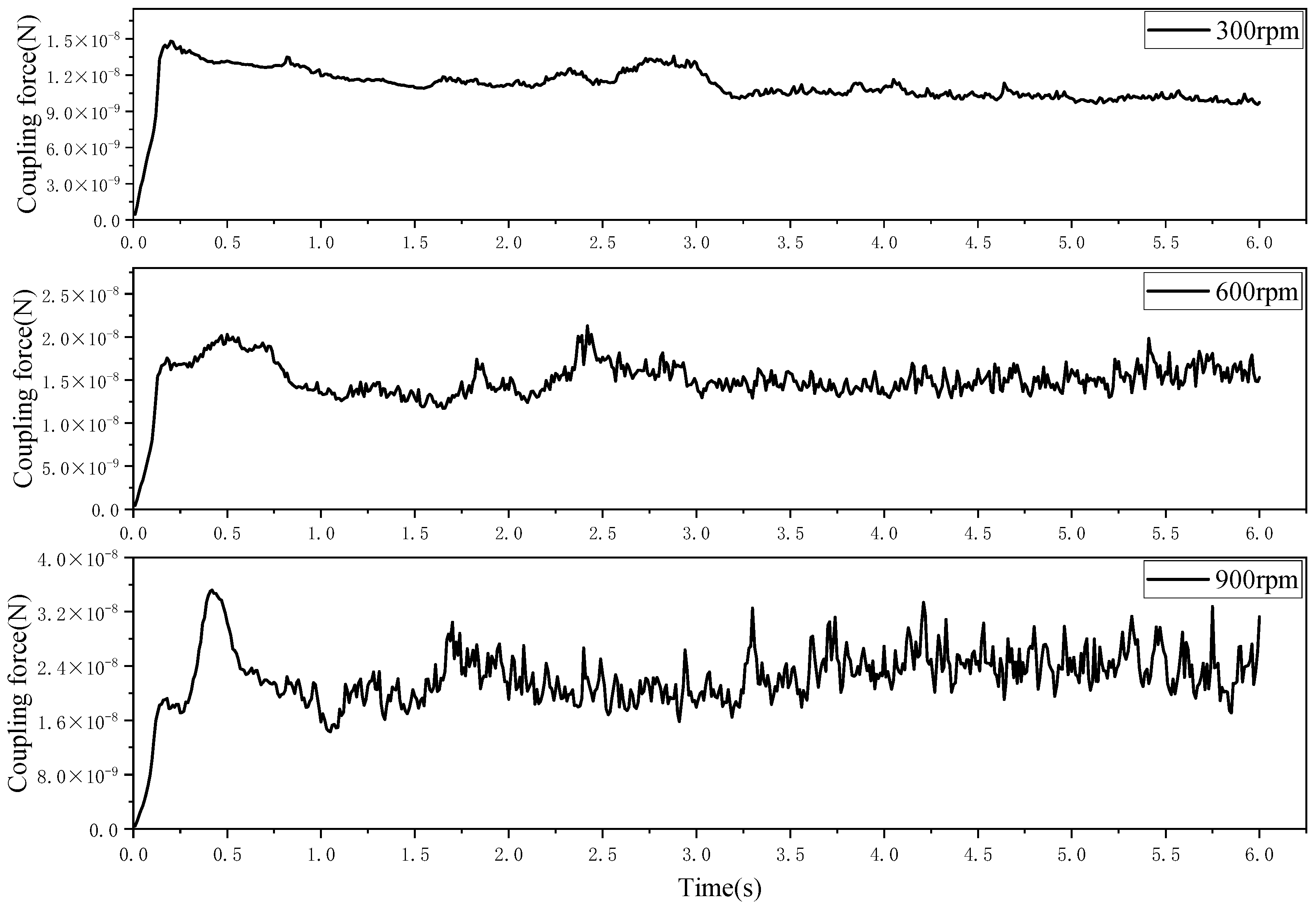
3.1.2. Impeller Speed Effects

The rotational speed of the agitator blade directly determines the flow field characteristics, turbulent intensity, and particle distribution/motion behavior in the tank. As shown in Figure 9, particle visualization reveals their positions at different times in the stirred tank: Initially, particles undergo free fall under gravity in the stirred tank. Upon contacting the aqueous phase, their descent velocity decreases due to hydrodynamic forces. Subsequently, as the agitator rotates, particles begin to disperse and migrate along the fluid flow direction. Upon colliding with the tank wall and baffles, particle motion transitions to axial motion. Due to the bidirectional flow characteristics along the baffles, a portion of particles enters upward-flowing regions, where they are subjected to upward fluid drag forces promoting their upward motion. During this process, particles further disperse and spread into a larger spatial range. Due to the fluid drag effect, the ascent velocity of particles is influenced by the fluid velocity. The other portion of particles enters the downward-flowing regions of the flow field, similarly subjected to fluid drag forces that cause their downward motion. Under the combined effect of gravity and fluid drag, particles gradually settle toward the tank bottom. Because particle density exceeds liquid density, gravity dominates their motion when particles enter downward-flowing regions and settle to the tank bottom. Upward fluid drag forces are insufficient to overcome gravitational effects, thus these settled particles will not be resuspended. As agitator rotational speed continually increases, the flow field’s drag effect on particles is significantly enhanced, leading to marked improvements in axial uniformity of particle distribution and strengthening of the particle motion cycle within the stirred tank.

As shown in Figure 10, at the 6-second mark, significant differences emerge in cross-sectional velocity and fluid phase volume distribution across different rotational speeds. At low speeds (300 rpm), overall velocity magnitudes in the tank are small, with high-velocity regions concentrated around the agitator blades. As rotational speed increases, velocity magnitudes rise significantly, and high-velocity zones expand, providing the fluid with increased kinetic energy and enhancing particle mixing. Low speeds of fluid phase volume distribution result in non-uniform distribution with distinct stratification and agglomeration. Conversely, higher speeds promote uniform fluid phase distribution, indicating that increased rotational speed effectively improves solid–liquid mixing efficiency and promotes homogeneous fluid phase distribution within the stirred tank.

To more accurately characterize particle motion under different rotational speeds, coupling forces are introduced to evaluate the forces acting on particles and determine when stable states are achieved. The coupling force is the resultant force of drag and lift forces, with drag force being dominant [33,34], using the Haider–Levenspiel drag force model and the Saffman lift force model. Figure 11 shows the curves of coupling force over time at different rotational speeds. It can be clearly observed from the curves that, after particles come into contact with the free liquid surface, their motion goes through three stages: sedimentation, dispersion, and circulation. During the initial stirring stage, eddies have not yet formed, and rotational speed has minimal impact on liquid turbulence. Consequently, average coupling forces during pull-downs show little fluctuation with varying speeds. However, significant changes occur during the dispersion and cycle stages. Higher rotational speeds strengthen eddy currents in the stirred tank, intensifying particle-fluid interactions and increasing average coupling forces. Notably, coupling forces rise continuously with increasing speed during the dispersion phase. This is primarily due to enhanced turbulence and vortex effects generated via higher speeds, leading to more frequent particle collisions and stronger interparticle interactions, which drive coupling force increases and more considerable amplitude variations during the cycle stage.

As a critical statistical measure of data dispersion, RSD plays a key role in indicating particle dispersion uniformity: smaller RSD values signify more uniform particle distribution. Higher rotational speeds induce intense shear and turbulence effects, accelerating particle suspension and dispersion within the stirred tank—a phenomenon strongly supported by Yang et al.’s research [35]. To determine the dispersion of particles in the stirred tank, the tank is divided into multiple volume units. By counting the number of particles in each unit, the average particle number and standard deviation at each time step are calculated, and the RSD value is obtained using Equation (8). Figure 12 compares RSD curves over mixing time for the PBT agitator at different rotational speeds. Low-speed (e.g., 300 rpm) curves exhibit more significant fluctuations, while high-speed (e.g., 1000 rpm) curves show reduced variability. This is because low speeds provide limited shear force and mixing capacity, leading to non-uniform material distribution and significant RSD fluctuations. Conversely, high speeds rapidly disrupt initial material stratification, promoting system homogeneity and smaller RSD variations. Although RSD values stabilize at all speeds, high rotational speeds yield lower steady-state RSD, indicating superior mixing uniformity. In contrast, low speeds result in higher steady-state RSD, reflecting incomplete mixing. Additionally, with increasing rotational speed, RSD values decreased by 25–40% during the stable phase. Increasing rotational speed reduces the time required to achieve homogeneity and lowers the final RSD value, demonstrating improved mixing efficiency.

In summary, the analysis of particle dynamics characteristics focused on investigating the effects of varying particle size and agitator rotational speed on particle motion. Small particles follow Stokes’s law during pull-down, with their low settling velocities dominated by liquid viscosity, making them prone to suspension and flow-following motion in turbulent regions. Conversely, large particles adhere to a modified form of Stokes’s law, where significant inertial effects weaken fluid entrainment, causing trajectory deviations from flow direction and preferential deposition near the tank bottom. Agitator rotational speed exerts a critical influence on flow field characteristics: increasing speed enhances fluid drag on particles, improves axial particle distribution uniformity, accelerates the motion cycle, and promotes homogeneous fluid phase mixing. Higher speeds generate intense vortex and turbulence effects, leading to elevated liquid levels, increased pull-down of particles at the tank bottom, and amplified coupling forces.

3.1.3. Time-Series Prediction

To improve real-time operational condition prediction in industrial systems, time-series prediction models are critical. Data calculated by the coupled model up to 6 s were used as the dataset, with 80% allocated to the training set and the remaining 20% to the test set. As a typical spatial feature extraction model, the core purpose of including CNN is to verify its effectiveness in predicting time series. Cheng et al. [20] performed a time-series prediction of pressure using six different ML algorithms to forecast future states one step ahead, reporting accuracy rankings as BP~RF > SVM > CNN~LSTM~RBF. This section focuses on the time-series prediction of average particle velocity within the stirred tank over 6 s, training different algorithms to obtain evaluation metrics. The first 4.8 s served as the training set, while the last 1.2 s were used for testing. The impact of hidden layer neuron count was systematically explored for BP networks. RMSE values were calculated for neurons ranging from 50 to 100, with the optimal hidden layer configuration selected based on the minimum RMSE. During algorithm training, multiple different algorithms were employed to train the model, and comprehensive, objective performance evaluations were conducted using corresponding metrics, yielding detailed performance comparisons across all algorithms.

As shown in

Table 2. Time-series prediction performance of different ML models.

Algorithm		R2	R	MAE	MBE	RMSE
BP	Training	0.99986	0.99993	0.00041121	9.7225 × 10−6	0.00055297
	Test	0.98006	0.98998	0.00046321	0.0002731	0.00058149
GA-BP	Training	0.99985	0.99992	0.00042824	4.2143 × 10−6	0.00056754
	Test	0.98223	0.99108	0.00043053	0.00024306	0.00054896
LSTM	Training	0.99838	0.99919	0.0014657	−2.604 × 10−5	0.001896
	Test	0.93115	0.96496	0.00092888	0.00080094	0.0010804
ELM	Training	0.99988	0.99994	0.00039456	9.5328 × 10−11	0.00051279
	Test	0.97688	0.98837	0.00050124	0.00022597	0.00062618
CNN	Training	0.99489	0.99744	0.0020812	−0.00086056	0.003366
	Test	0.92587	0.96222	0.00088106	0.00066994	0.0011212
SVM	Training	0.99986	0.99993	0.00041974	−3.8306 × 10−5	0.00055695
	Test	0.97067	0.98523	0.00057967	0.00048397	0.0007052

, a quantitative analysis of prediction results using evaluation metrics reveals that BP demonstrates superior goodness of fit and error performance compared to other algorithms. Also, GA-optimized BP outperforms the original BP regarding R², MAE, MBE, and RMSE. This indicates that GA optimization effectively improves BP performance, enhancing the model’s fitting accuracy on the training set and also significantly boosting its generalization capability on the test set—enabling more accurate predictions for unseen data. However, this algorithm’s high computational cost renders it unsuitable for industrial real-time prediction requirements. Although ELM and SVM exhibit slightly lower performance than BP, their significantly faster computation speeds and R values > 0.98 meet most industrial needs.

As shown in

Table 3. Summary of time-series predictions of different ML models.

Algorithm	Core Mechanism	Difference in R	Advantages	Disadvantages	Applicable Scenarios
BP	Optimizing weights through backpropagation [36]	0.00995	Strong non-linear fitting ability and low error	Prone to getting stuck in local optima	Complex non-linear modeling
GA-BP	Optimizing initial weights using genetic algorithms [37]	0.00884	High fitting accuracy and strong generalization ability	High computational cost and requires GA optimization	Scenarios with high-precision requirements
LSTM	Capturing time-series dependencies via gating mechanisms [38]	0.03423	Good at capturing long-term dependencies in time-series data	Relatively large actual error	Short-term time-series prediction
ELM	Randomly initializing weights [39]	0.01157	No need for iterative parameter tuning and fast training speed	Limited generalization ability	Real-time response for condition monitoring
CNN	Handling spatial features [40]	0.03522	Good at processing spatial features	Poorest fitting degree	Edge detection in flow field graphics
SVM	Minimizing risk [41]	0.0147	Balancing accuracy and efficiency	Increasing computational complexity	Data evaluation for dynamic response

, a qualitative analysis is conducted on the prediction results of different algorithms. In terms of generalization performance, GA-BP and BP, with their weight optimization mechanisms, exhibit the closest performance between the training set and the test set, indicating strong generalization ability. ELM and SVM achieve medium-level generalization performance. ELM relies on randomly initialized weights, enabling fast training but with limited generalization. SVM balances accuracy and efficiency through risk minimization, yet its computational complexity increases with the data scale, and it can quickly respond to condition monitoring. ELM strikes a balance between training efficiency and computational cost. It does not require iterative parameter tuning and directly solves the problem after randomly initializing the weights, so it has the fastest training speed and is suitable for real-time or fast-response scenarios. GA-BP combines a genetic algorithm to optimize the initial weights, which requires an additional GA iteration process, resulting in the highest computational cost. It is suitable for scenarios with extremely high precision requirements where a long training time is acceptable.

A visual evaluation of the predictions is conducted through Figure 13 and Figure 14. Figure 13 illustrates the error changes of the prediction models at different times. Figure 13a shows the prediction performance over the entire time period, indicating that the adopted models have relatively accurate prediction capability for time-series data. Figure 13b,c display the results of the last 1.2 s of the test set prediction, revealing that GA-BP, BP, and ELM exhibit higher fitting degrees with the true values and greater prediction accuracy compared to other algorithms. Figure 14 presents scatter plots of the correlation between predicted and true values for different algorithms. The more densely the scatter points are distributed around the fitted curve, the smaller the deviation between the model’s predictions and the true values. A 95% confidence interval is also plotted to further reflect the stability of model predictions—narrower intervals indicate smaller fluctuations and better stability in predicted values. The results show that the scatter points of BP, GA-BP, and ELM are most uniformly distributed around the fitted curve. Among them, GA-BP has a relatively narrower confidence interval, demonstrating not only high accuracy but also good stability. In contrast, LSTM and CNN algorithms show scattered scatter points and wider confidence intervals, indicating larger fluctuations and poorer stability in their predictions. These findings further validate the accuracy and stability of the GA-BP algorithm.

In summary, six algorithms were compared in terms of time-series prediction accuracy for stirred tanks: GA-BP > BP > ELM > SVM > LSTM > CNN. GA-BP and BP significantly outperform other models in fitting accuracy, while ELM and SVM balance efficiency and accuracy, and LSTM and CNN exhibit weaker performance.

3.2. Mass Transfer

As direct determinants of stirred tank dynamics, mass transfer processes typically involve substance dissolution from solid particle surfaces into liquids or adsorption of liquid-phase substances onto solid surfaces. Fluid flow characteristics, solid–liquid interfacial contact area, and interphase concentration gradients influence mass transfer rates. When studying mass transfer processes, the mass transfer coefficient k is a critical parameter for quantifying transfer rates. To accurately determine this parameter, In the research of this section, key parameters such as flow field velocity and particle motion are first obtained through CFD-DEM two-way coupling simulation. Then, a calculation framework for the key parameter Sh of the mass transfer process is constructed based on the Hughmark model. Here, Sc is set to 0.7 according to the Standard k-ε model to ensure the accuracy and reliability of the entire mass transfer process calculation. Further, combined with the definition of Re in Formulas (9) and (10), the Re value is calculated through the relative velocity of the solid–liquid two-phase and the physical property parameters of the fluid. Finally, the quantitative solution of k is completed based on the correlation between Sh, Re, and Sc. The calculated k values were validated against experimental results from Carletti et al. [42]. To achieve real-time prediction of mass transfer coefficients, different ML algorithms were employed for predictive analysis.

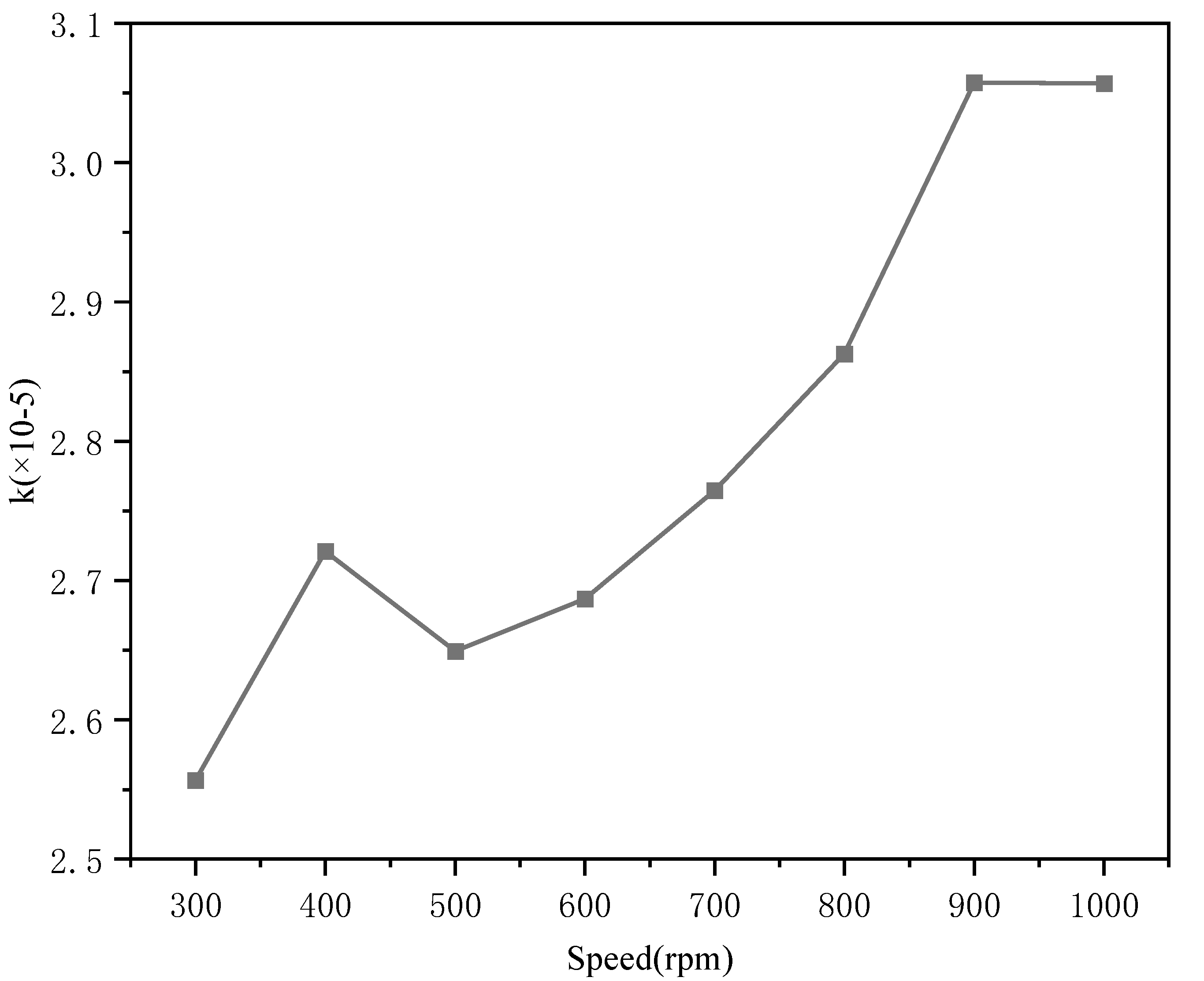
3.2.1. Speed Dependency

According to Liu et al. [43], the mechanism by which rotational speed influences mass transfer coefficients is closely linked to particle motion characteristics. Their rotating packed bed (RPB) experiments revealed that increasing rotational speed from 200 rpm to 2200 rpm significantly enhanced k values, attributed to intensified shear forces and turbulence between liquid and particles—thereby promoting solid–liquid interface renewal and ion exchange rates. Li et al. [34] investigated the effect of rotational speed on particle dispersion in a stirred tank. The translational kinetic energy increases significantly with increasing rotational speed, as high-speed flow imparts more linear momentum to the particles. In contrast, the rotational kinetic energy reaches its maximum at moderate rotational speeds: at low speeds, the fluid driving force is insufficient, while at high speeds, the complex dynamic motion of particles inhibits further increases in rotational kinetic energy, leading to an increase in particle concentration at the bottom of the tank.

This study investigated the effect of PBT agitator rotational speeds (300–1000 rpm) on k values, finding that k generally increased with higher speeds. This indicates that enhanced agitation at elevated speeds promotes material transport, leading to more significant mass transfer coefficients. As presented in

Table 4. Calculated mass transfer coefficients for the PBT agitator at different rotational speeds.

Rotational Speed (rpm)	Fluid Velocity (m/s)	Particle Velocity (m/s)	Relative Velocity (m/s)	Re	k (×10−5)
300	0.0847	0.0738	0.0110	1.0913	2.5565
400	0.1058	0.0874	0.0184	1.8309	2.7209
500	0.1433	0.1283	0.0149	1.4854	2.6493
600	0.1733	0.1900	0.0167	1.6616	2.6867
700	0.1985	0.2192	0.0207	2.0510	2.7645
800	0.2318	0.2581	0.0263	2.6219	2.8626
900	0.2526	0.2922	0.0396	3.9400	3.0575
1000	0.2593	0.2989	0.0395	3.9345	3.0567

and Figure 15, before the rotational speed reaches 500 rpm, particle velocity remains slightly lower than fluid velocity. At this stage, pull-down dominates due to high particle inertia (elevated Stokes number), preventing full fluid-particle motion synchronization at low speeds. This results in reduced mass transfer efficiency and correspondingly low k values. As the speed increases, particle velocity surpasses fluid velocity, with relative velocity and Re fluctuating upward (Re rising from 1.48 to 3.94). Enhanced slip effects and turbulent vortices accelerate interfacial renewal, driving k to its peak. Further speed increases improve particle followability, causing localized turbulent kinetic energy dissipation and declining mass transfer efficiency. Excessively high speeds may induce centrifugal particle aggregation or circulation, reducing central region particle concentration and effective mass transfer area—ultimately decreasing k.

In analyzing mass transfer processes for the PBT agitator, the study focused on the effects of agitator rotational speed and solid concentration on the mass transfer coefficient between suspended particles and fluid. The results show that k generally increases with rising rotational speed. However, the relative velocity between particles and fluid significantly influences mass transfer efficiency. At low speeds, high particle inertia restricts improvements in mass transfer efficiency. In medium speed ranges, turbulence enhancement dominates, effectively promoting mass transfer. Mass transfer efficiency declines at high speeds due to improved particle followability and centrifugal effects. Therefore, optimizing mass transfer performance requires balancing agitation intensity with particle response characteristics.

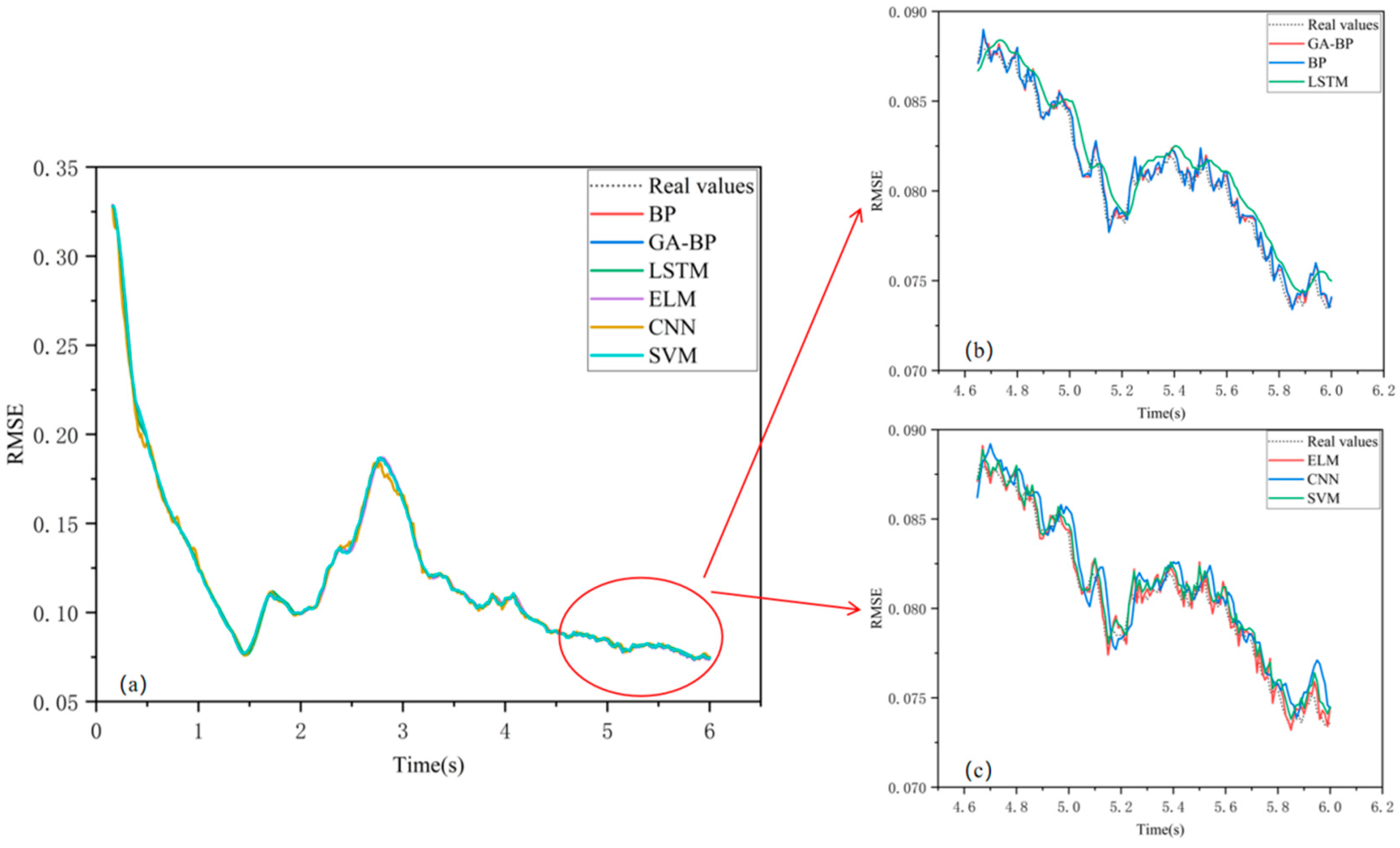
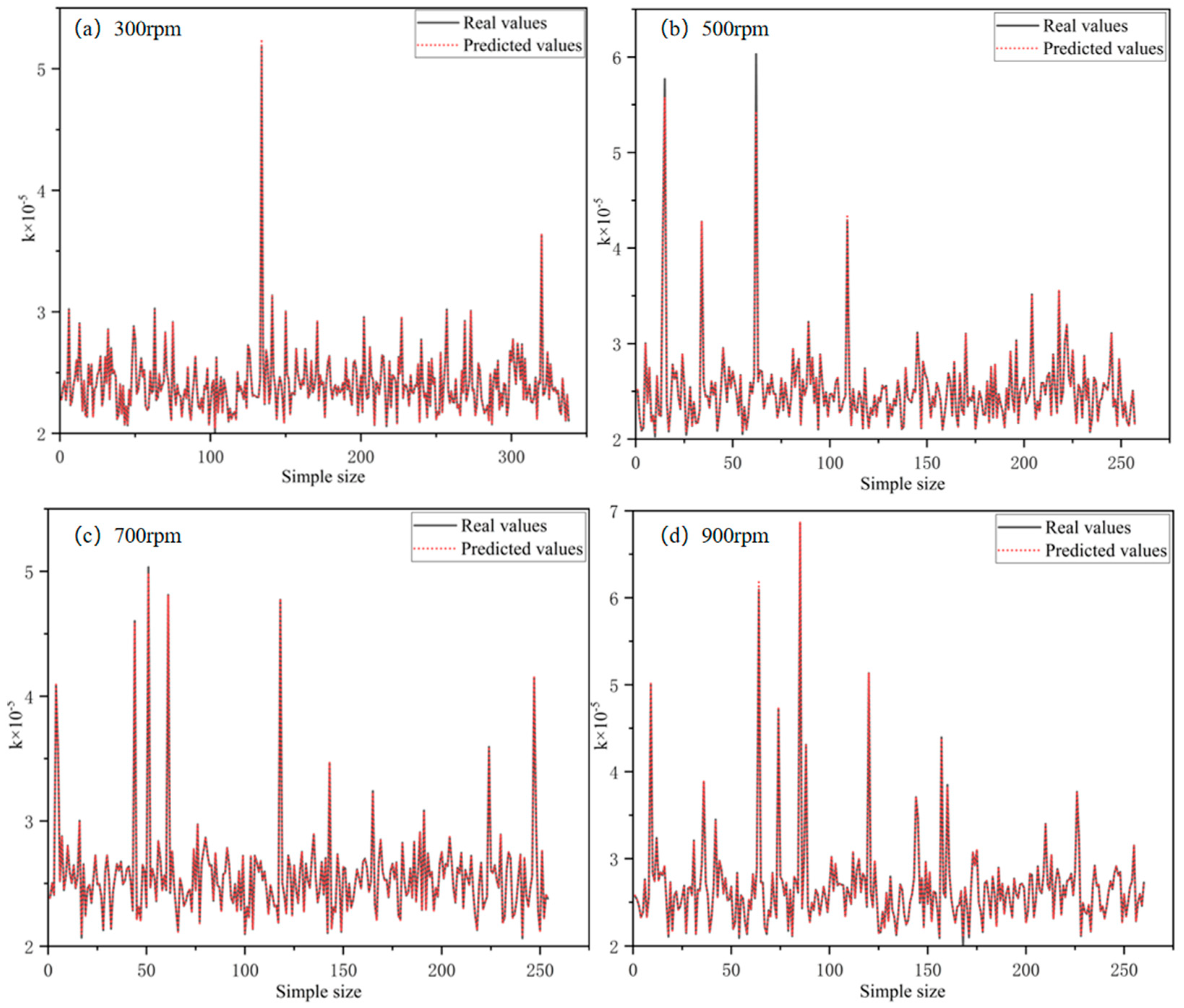
3.2.2. ML Prediction

This section’s study selected the spatial positions of particles and slip velocities as input variables, with k as the output variable, to construct the dataset. The dataset contained 1700 samples, with 80% divided into the training set for model training and parameter optimization and the remaining 20% serving as the test set to evaluate model generalization ability and prediction accuracy. Hyperparameters included 5000 iterations, an error threshold 1 × 10⁻⁶, and a learning rate of 0.01. To ensure reliability, reproducibility, and fair comparisons between algorithms, a fixed random seed method was adopted, with the initial values and hyperparameters kept consistent across all training runs.

As shown in

Table 5. Performance comparison of different ML models.

Algorithms		R2	R	MAE	MBE	RMSE
BP	Training	0.99973	0.99986	0.0014704	−7.6856 × 10−5	0.0034852
	Test	0.98416	0.99205	0.0033053	0.0014924	0.032499
GA-BP	Training	0.99987	0.99993	0.0013553	5.9696 × 10−5	0.0023766
	Test	0.99987	0.99993	0.001514	−6.8653 × 10−5	0.0029763
RF	Training	0.99564	0.99782	0.0031699	−0.00037206	0.013898
	Test	0.88701	0.94181	0.01091	−0.0058259	0.08679
XGBoost	Training	0.99996	0.99998	0.001001	2.2163 × 10−7	0.0013082
	Test	0.95656	0.97804	0.0047947	−0.0035598	0.053812
LSTM	Training	0.94695	0.97311	0.037583	−7.5798 × 10−5	0.048483
	Test	0.91935	0.95883	0.041425	−0.0017029	0.073324
ELM	Training	0.93725	0.96812	0.038562	−4.274 × 10−7	0.052728
	Test	0.93885	0.96894	0.041769	−0.0012613	0.063845
CNN	Training	0.97488	0.98736	0.022713	0.017768	0.033362
	Test	0.97206	0.98593	0.024634	0.018	0.043157
SVM	Training	0.96065	0.98013	0.0295	0.0046757	0.041754
	Test	0.95176	0.97558	0.034408	0.0046691	0.056709

, regarding the performance of different ML models. In terms of prediction accuracy, GA-BP achieves high and identical R values in both the training and test sets, outperforms other algorithms, and demonstrates the highest prediction accuracy. CNN also met high accuracy demands, making it suitable for flow prediction in this model. RF showed excellent training set performance but significant overfitting (large training-test discrepancy), rendering it unsuitable for flow prediction. Regarding error evaluation: XGBoost had the smallest MAE on the training set, and BP had the smallest RMSE. On the test set, BP again demonstrated stronger error control with smaller MAE and RMSE. However, LSTM and ELM exhibited relatively large error metrics on both datasets, indicating lower model accuracy.

Table 6. Summary of mass transfer coefficient predictions by different ML models.

Algorithm	Core Mechanism	Difference in R	Advantages	Disadvantages	Applicable Scenarios
BP	Multivariate non-linear mapping	0.00781	Stable error control	Slow training	Modeling of complex mass transfer processes
GA-BP	Enhanced generalization ability after optimization	0	Strong fitting and generalization ability	High computational cost	High-precision prediction of mass transfer coefficients
RF	Ensemble of decision trees for feature selection [44]	0.05601	Parallel processing of high-dimensional data	Severe overfitting	Rapid response for feature selection
XGBoost	Gradient boosting for anti-overfitting [45]	0.02194	Strong anti-overfitting ability	Requires fine-tuning of parameters	Rapid data deployment
LSTM	Gating mechanism to capture time-series dependencies	0.01428	Alleviates gradient vanishing	Large prediction error	Analysis of mass transfer fluctuations
ELM	Random weights for rapid solution	0.00082	Fast training speed	Weak generalization ability	Rapid mass transfer prediction
CNN	Incorporating particle spatial distribution for auxiliary prediction	0.00143	Extracts spatial features and non-linear relationships	High demand for computational resources	Mass transfer prediction with spatial features
SVM	Risk minimization	0.00455	Balances accuracy and efficiency	Difficult to select kernel functions	Evaluation of mass transfer efficiency

summarizes the prediction of mass transfer coefficients via different algorithms. GA-BP achieves an ideal state with a difference in R of 0, indicating that its performance in the training set and test set is exactly consistent without overfitting. Its core advantage is the significant enhancement of generalization ability through genetic algorithm optimization, making it suitable for high-precision prediction of mass transfer coefficients. Next, ELM relies on randomly initialized weights for a rapid solution, enabling extremely fast and high-precision prediction in scenarios with small-scale data or simple mass transfer processes. CNN, by incorporating the spatial distribution characteristics of particles, demonstrates outstanding fitting capability for mass transfer data containing spatial information. In terms of efficiency, SVM’ s computational complexity depends on kernel functions, XGBoost requires parameter tuning for optimization, and LSTM is constrained by the iterative calculation of its gating mechanism—all limiting their efficiency. Although RF exhibits the poorest fitting degree, its feature selection capability allows it to be used for high-dimensional feature screening of mass transfer data, assisting other models in completing predictions.

Figure 16 indicates that under different rotational speeds, the fluctuation patterns of predicted and valid values are in good agreement, with nearly identical deviation magnitudes. This demonstrates that the GA-BP algorithm can effectively capture data variation laws across diverse rotational speed conditions and exhibits robust stability.

Regarding the real-time prediction accuracy of mass transfer coefficients, a comparative analysis of eight algorithms shows the following order: GA-BP > BP > CNN > XGBoost > SVM > ELM > LSTM > RF. Furthermore, the GA-BP algorithm demonstrates high matching degree between predicted and true values under different rotational speeds, stable deviation, and strong adaptability to multiple operating conditions, thereby exhibiting excellent stability.

4. Conclusions

This study constructed a CFD-DEM coupling model integrated with a machine learning framework to analyze particle motion and mass transfer characteristics in solid–liquid stirred tanks and predict parameters. The main conclusions are as follows: particle size significantly influences their motion behavior—reducing particle size facilitates particle suspension in the tank. Increasing the impeller rotational speed enhances particle circulatory motion, shortens mixing time, and decreases the RSD value by 25–40%. The coupling force acting on particles increases with higher rotational speeds, while the stability during the circulation stage deteriorates. In the mass transfer process, the mass transfer coefficient k generally exhibits an upward trend as the rotational speed increases. In terms of parameter prediction, for time-series prediction of particle motion, the algorithm performance ranks as follows: GA-BP > BP > ELM > SVM > LSTM > CNN. For the real-time prediction of mass transfer coefficients, the ranking is as follows: GA-BP > BP > CNN > XGBoost > SVM > ELM > LSTM > RF. The GA-BP algorithm achieves an R fitting degree of 0.99 in predictions, and its stability under different operating conditions has also been validated. This study provides theoretical support for the structural optimization and intelligent control of stirred tanks, promoting the deep integration of multiphase flow research with artificial intelligence technologies.

In future research on solid–liquid stirred tanks, the integration of DeepLab, EfficientNet, and PIV technology can provide more accurate experimental validation for CFD-DEM simulations. Through in-depth analysis of PIV images, this approach can not only validate the accuracy of simulations but also uncover complex physical phenomena that simulations have not considered, thereby guiding the direction for model improvement and optimization. This synergy will promote more efficient and precise development of related research.

References

1. Peng, H.; Zhou, Q.; Liu, H.P.; Huang, X.Y.; Liu, Y.L.; Ran, C.E.; Pan, W.J. Research Progress on Vanadium Extraction Technology from Vanadium Slag. Acta. Petrol. Mineral. 2025, 44, 216–226. [Google Scholar]
2. Gharabaghi, M.; Azadmehr, A.; Aghazadeh, S.; Pourabdoli, M. Clean Practical Method for Cadmium Recycling from Toxic Material and Optimization of Recycling Process. JOM 2022, 74, 1945–1957. [Google Scholar] [CrossRef]
3. Karacahan, M.K. Optimization and Kinetic Study of Manganese Leaching from Pyrolusite Ore in Hydrochloric Acid Solutions with Oxalic Acid. J. Sustain. Met. 2024, 10, 1717–1732. [Google Scholar] [CrossRef]
4. Ismail, N.I.; Kuang, S.; Yu, A. CFD-DEM study of particle-fluid flow and retention performance of sand screen. Powder Technol. 2021, 378, 410–420. [Google Scholar] [CrossRef]
5. Gu, D.; Ye, M.; Liu, Z. Computational fluid dynamics simulation of solid-liquid suspension characteristics in a stirred tank with punched circle package impellers. Int. J. Chem. React. Eng. 2020, 18, 20200026. [Google Scholar] [CrossRef]
6. Xia, D.; Mao, Z.J.; Zhou, S.Q.; He, X.; Wang, Y.X. Optimized Design of Solid-Liquid Dual-Impeller Mixing Systems for Enhanced Efficiency. ACS Omega 2023, 8, 47635–47645. [Google Scholar] [CrossRef]
7. Kohnen, C.; Bohnet, M. Measurement and simulation of fluid flow in agitated solid/liquid suspensions. Chem. Eng. Technol. 2001, 24, 639–643. [Google Scholar] [CrossRef]
8. Gu, D.; Li, C.; Gu, X.; Wang, J. Solid-liquid mixing characteristics in a fractal cut impeller stirred reactor with dense solid loading. Chem. Eng. Process.-Process. Intensif. 2024, 196, 109655. [Google Scholar] [CrossRef]
9. Sommer, A.E.; Rox, H.; Shi, P.; Eckert, K.; Rzehak, R. Solid-liquid flow in stirred tanks: “CFD-grade” experimental investigation. Chem. Eng. Sci. 2021, 245, 116743. [Google Scholar] [CrossRef]
10. Gu, D.; Xu, H.; Ye, M.; Wen, L. Design of impeller blades for intensification on fluid mixing process in a stirred tank. J. Taiwan Inst. Chem. Eng. 2022, 138, 104475. [Google Scholar] [CrossRef]
11. Hu, Y.; Zhang, Y.M.; Xue, N.N.; Zheng, Q. Numerical Simulation of Solid-Liquid Mixing Characteristics of Vanadium Shale with Stirring Tank Shape. Nonferrous Met. (Extr. Metall.) 2022, 11, 68–77. [Google Scholar]
12. Basheer, A.A.; Bharathesh, K. Effect of baffle configuration on hydrodynamics and solid suspension in a continuous stirred vessel. Chem. Eng. Commun. 2021, 209, 1413–1422. [Google Scholar] [CrossRef]
13. Li, S.; Yang, R.; Wang, C.; Shen, Y.; Wang, H. Simulation of the solid particles behavior in 3D stirred tank using CFD-DEM coupling approach. Part. Sci. Technol. 2022, 40, 911–921. [Google Scholar] [CrossRef]
14. Luo, X.; Yu, J.; Wang, B.; Wang, J. Heat Transfer and Hydrodynamics in Stirred Tanks with Liquid-Solid Flow Studied by CFD–DEM Method. Processes 2021, 9, 849. [Google Scholar] [CrossRef]
15. Wu, Y.K.; Li, Z.Q.; Wang, Y.; Xu, Z.; Li, K.; Shi, H. Research on Stirring Process Based on Artificial Neural Network and Multi-Phase Flow Simulation Technology. Nonferrous Met. Sci. Eng. 2024, 15, 801–813. [Google Scholar]
16. Choong, C.E.; Ibrahim, S.; El-Shafie, A. Artificial Neural Network (ANN) model development for predicting just suspension speed in solid-liquid mixing system. Flow Meas. Instrum. 2020, 71, 101689. [Google Scholar] [CrossRef]
17. Moya, J.D.; Molina, A.E.; Belmonte, J.F.; Córcoles-Tendero, J.I.; Almendros-Ibáñez, J.A. Characterization of a triple concentric-tube heat exchanger with corrugated tubes using Artificial Neural Networks (ANN). Appl. Therm. Eng. 2019, 147, 1036–1046. [Google Scholar] [CrossRef]
18. Joshi, S.S.; Dalvi, V.H.; Vitankar, V.S.; Joshi, A.J.; Joshi, J.B. Novel Correlation for the Solid–Liquid Mass Transfer Coefficient in Stirred Tanks Developed by Interpreting Machine Learning Models Trained on Literature Data. Ind. Eng. Chem. Res. 2023, 62, 19920–19935. [Google Scholar] [CrossRef]
19. Zhao, X.; Fan, H.; Lin, G.; Fang, Z.; Yang, W.; Li, M.; Wang, J.; Lu, X.; Li, B.; Wu, K.; et al. Multi-objective optimization of radially stirred tank based on CFD and machine learning. AIChE J. 2023, 70, 18324. [Google Scholar] [CrossRef]
20. Cheng, H.; Liu, Z.; Li, S.; Du, Y. Machine learning analysis of pressure fluctuations in a gas-solid fluidized bed. Powder Technol. 2024, 444, 120065. [Google Scholar] [CrossRef]
21. Song, Z.; Zou, S.; Zhou, W.; Huang, Y.; Shao, L.; Yuan, J.; Gou, X.; Jin, W.; Wang, Z.; Chen, X.; et al. Clinically applicable histopathological diagnosis system for gastric cancer detection using deep learning. Nat. Commun. 2020, 11, 4294. [Google Scholar] [CrossRef]
22. Kabir, H.; Wu, J.; Dahal, S.; Joo, T.; Garg, N. Automated estimation of cementitious sorptivity via computer vision. Nat. Commun. 2024, 15, 9935. [Google Scholar] [CrossRef]
23. Puderbach, V.; Schmidt, K.; Antonyuk, S. A Coupled CFD-DEM Model for Resolved Simulation of Filter Cake Formation during Solid-Liquid Separation. Processes 2021, 9, 826. [Google Scholar] [CrossRef]
24. Jovanović, A.; Pezo, M.; Pezo, L.; Lević, L. DEM/CFD analysis of granular flow in static mixers. Powder Technol. 2014, 266, 240–248. [Google Scholar] [CrossRef]
25. Jiang, H.; Yuan, S.; Liu, H.; Li, W.; Zhou, X. Numerical analysis and optimization of key parts in the stirred tank based on solid-liquid flow field. Sci. Prog. 2022, 105, 1–26. [Google Scholar] [CrossRef]
26. Trinh, C.; Meimaroglou, D.; Hoppe, S. Machine Learning in Chemical Product Engineering: The State of the Art and a Guide for Newcomers. Processes 2021, 9, 1456. [Google Scholar] [CrossRef]
27. Wu, Y.; Li, Z.; Zhang, B.; Chen, H.; Sun, Y. Multi-objective optimization of key parameters of stirred tank based on ANN-CFD. Powder Technol. 2024, 441, 119832. [Google Scholar] [CrossRef]
28. Raikov, A.N.; Panfilov, S.A. Convergent Decision Support System with Genetic Algorithms and Cognitive Simulation. IFAC Proc. Vol. 2013, 46, 1108–1113. [Google Scholar] [CrossRef]
29. Zhang, J.; Qu, S.; Lv, Z. Optimization of Backpropagation Neural Network under the Adaptive Genetic Algorithm. Complexity 2021, 2021, 1718234. [Google Scholar] [CrossRef]
30. Raissi, M.; Yazdani, A.; Karniadakis, G.E. Hidden fluid mechanics: Learning velocity and pressure fields from flow visualizations. Science 2020, 367, 1026–1030. [Google Scholar] [CrossRef]
31. Cuomo, S.; Di Cola, V.S.; Giampaolo, F.; Rozza, G.; Raissi, M.; Piccialli, F. Scientific Machine Learning Through Physics–Informed Neural Networks: Where we are and What’s Next. J. Sci. Comput. 2022, 92, 88. [Google Scholar] [CrossRef]
32. Hornik, K.; Stinchcombe, M.; White, H. Multilayer feedforward networks are universal approximators. Neural Netw. 1989, 2, 359–366. [Google Scholar] [CrossRef]
33. Kang, Q.; Feng, X.; Yang, C.; Wang, J. DEM-VOF simulations on the drawdown mechanisms of floating particles at free surface in turbulent stirred tanks. Chem. Eng. J. 2022, 431, 133275. [Google Scholar] [CrossRef]
34. Li, M.; Zhang, L.; Li, C.; Wu, G.; An, X.; Zhang, H.; Fu, H.; Yang, X.; Zou, Q. Discrete Element Method–Volume of Fluid Simulation of Drawdown and Dispersion for Floating Particles in Stirred Tanks: Influences of Impeller Parameters. Ind. Eng. Chem. Res. 2024, 63, 10353–10372. [Google Scholar] [CrossRef]
35. Yang, F.; Zhang, C.; Sun, H.; Liu, W. Solid-liquid suspension in a stirred tank driven by an eccentric-shaft: Electrical resistance tomography measurement. Powder Technol. 2022, 411, 117943. [Google Scholar] [CrossRef]
36. Rumelhart, D.E.; Hinton, G.E.; Williams, R.J. Learning representations by back-propagating errors. Nature 1986, 323, 533–536. [Google Scholar] [CrossRef]
37. Wang, Q.Q.; An, A.M.; Tang, M.A.; Liu, J. Distributed nonlinear model predictive control for cobalt removal process in zinc hydrometallurgy considering error compensation modelling. Can. J. Chem. Eng. 2024, 102, 307–323. [Google Scholar] [CrossRef]
38. Christudas, F.; Dhanraj, A.V. System Identification Using Long Short Term Memory Recurrent Neural Networks for Real Time Conical Tank System. Rom. J. Inf. Sci. Technol. 2020, 23, T57–T77. [Google Scholar]
39. Huang, G.-B.; Zhu, Q.-Y.; Siew, C.-K. Extreme learning machine: Theory and applications. Neurocomputing 2006, 70, 489–501. [Google Scholar] [CrossRef]
40. Hoseini, S.; Rundquist, E.; Poux, M.; Aubin, J. Foam detection in a stirred tank using deep learning neural networks. Chem. Eng. Res. Des. 2024, 209, 346–357. [Google Scholar] [CrossRef]
41. Zhong, W.M.; He, G.L.; Pi, D.Y.; Sun, Y.X. SVM with quadratic polynomial kernel function based nonlinear model one-step-ahead predictive control. Chin. J. Chem. Eng. 2005, 13, 373–379. [Google Scholar]
42. Carletti, C.; Bikić, S.; Montante, G.; Paglianti, A. Mass Transfer in Dilute Solid-Liquid Stirred Tanks. Ind. Eng. Chem. Res. 2018, 57, 6505–6515. [Google Scholar] [CrossRef]
43. Liu, B.; Dong, K.; Chen, R.-J.; Chang, S.-T.; Chu, G.-W.; Zhang, L.-L.; Zou, H.-K.; Sun, B.-C. Study on the Solid–Liquid Mass-Transfer Performance of Suspension in a Rotating Packed Bed. Ind. Eng. Chem. Res. 2023, 62, 8063–8070. [Google Scholar] [CrossRef]
44. Moholkar, C.D.; Vala, S.V.; Mathpati, C.S.; Joshi, A.J.; Vitankar, V.S.; Joshi, J.B. Artificial intelligence-based correlation: Process side heat transfer coefficient for helical coils in stirred tank reactors. Heat Transf. 2022, 51, 3099–3125. [Google Scholar] [CrossRef]
45. Zhang, Z.F.; Huang, Y.M.; Qin, R.; Ren, W.; Wen, G. XGBoost-based on-line prediction of seam tensile strength for Al-Li alloy in laser welding: Experiment study and modelling. J. Manuf. Process. 2021, 64, 30–44. [Google Scholar] [CrossRef]
Figure 1. Technical route.
Processes 13 01423 g001
Figure 2. Structure and dimensions of the stirred tank and impeller.
Processes 13 01423 g002
Figure 3. Physical model of the stirred tank.
Processes 13 01423 g003
Figure 4. Grid independence calculation results: curve of velocity magnitude variation near the impeller.
Processes 13 01423 g004
Figure 5. ANN algorithm network structures: (a) BP (backpropagation); (b) CNN (convolutional neural network); (c) LSTM (long short-term memory); (d) ELM (extreme learning machine).
Processes 13 01423 g005
Figure 6. Flow chart of GA-Optimized BP.
Processes 13 01423 g006
Figure 7. The performance of different training algorithms varies, depending on the number of neurons.
Processes 13 01423 g007
Figure 8. Trajectories of particles of different sizes in a stirred tank: (a) 1 mm; (b) 500 μm; (c) 100 μm.
Processes 13 01423 g008
Figure 9. The dispersion process of small particles over time at different rotational speeds: (a) 300 rpm; (b) 600 rpm; (c) 900 rpm.
Processes 13 01423 g009
Figure 10. Cross-sectional velocity and fluid phase volume changes at different rotational speeds at the 6 s mark: (a) 300 rpm; (b) 600 rpm; (c) 900 rpm.
Processes 13 01423 g010
Figure 11. Coupling forces over time at different rotational speeds.
Processes 13 01423 g011
Figure 12. RSD over time at different rotational speeds for the PBT agitator.
Processes 13 01423 g012
Figure 13. Prediction performance of different algorithms: (a) RMSE overtime for all algorithms during the 6 s period; (b,c) predictions over time for different algorithms after 4.8 s.
Processes 13 01423 g013
Figure 14. Correlation between predicted and real values for different algorithms: (a) GA-BP; (b) BP; (c) LSTM; (d) ELM; (e) CNN; (f) SVM. Blue circles represent the 95% confidence interval range, and red circles represent the interval vertices.
Processes 13 01423 g014
Figure 15. The variation of the mass transfer coefficient for the PBT impeller with rotational speed.
Processes 13 01423 g015
Figure 16. Comparison of predicted and true values of the training set using GA-BP at different rotational speeds: (a) 300 rpm; (b) 500 rpm; (c) 700 rpm; (d) 900 rpm.
Processes 13 01423 g016