Article

Accuracy Analysis of Slurry Characterization in a Rectifying Liquid Concentration Detection System

School of Materials Science and Engineering, Anhui University of Science and Technology, Huainan 232001, China
*
Author to whom correspondence should be addressed.
Processes 2025, 13(5), 1421; https://doi.org/10.3390/pr13051421
Submission received: 29 March 2025 / Revised: 25 April 2025 / Accepted: 4 May 2025 / Published: 7 May 2025
(This article belongs to the Section Chemical Processes and Systems)

Abstract

:
Accurately detecting coal slime water concentration during coal washing is crucial for optimizing dosing systems and improving separation efficiency. Traditional concentration detection methods are often affected by flow field disturbances. To address these limitations, this paper proposes a pressure differential concentration detection system utilizing interference rectification for a stabilized flow field and improved measurement accuracy. The experimental system comprises a circulating slurry tank, a defoamer, and a turbulence removal measuring tank. Numerical simulations and experimental studies investigated the effects of slurry concentration and inflow velocity on detection accuracy. Through dynamic measurement of pressure difference data under different concentrations and flow rates, the characteristics of a solid–liquid two-phase flow field are simulated using Fluent software. The results demonstrate that for low-concentration (C = 10%) and high-concentration (C = 30%) slurries, a flow velocity of ≥0.7 m/s significantly improves flow uniformity and achieves a stable particle suspension state, maintaining a measurement error within 1% for a flow rate of 0.7 m/s. However, flow rates exceeding 0.7 m/s decrease flow stability, increasing errors. Notably, the combination of sensors at positions No. 2 and No. 4 yields the lowest measurement errors, which verifies the influence of sensor layout on detection accuracy. A 0.7 m/s velocity is identified as the key threshold for flow field stability, and the nonlinear influence of the synergistic effect of flow rate and concentration on the detection stability is revealed. These findings provide valuable insights for optimizing pulp concentration detection systems and enhancing industrial dosing precision.

1. Introduction

A large amount of slime water [1,2,3] is produced during coal washing and processing. In coal preparation plants, the dosing system in the concentration link is crucial, as it directly influences the quality of the overflow circulating water, the efficiency of tailing slime press filtration and dehydration, and ultimately the separation process [4,5]. At a given flow rate, an excessively high concentration combined with insufficient dosage can lead to turbid overflow water from the concentration pool, preventing it from meeting the coal washing plant’s circulating water standards. In addition, poor coal slime sedimentation negatively influences the subsequent filtration and dewatering process. Conversely, if the concentration is too low, excessive chemical dosing may occur, leading to chemical waste and leaving high residual chemical content in the overflow water, which can affect flotation performance [6,7,8]. Therefore, accurately measuring coal slime water concentration and flow rate is essential for establishing an efficient dosing system, ensuring accurate chemical dosing. Currently, flow detection predominantly relies on electromagnetic flowmeters, which are technologically mature, along with the non-full-tube flowmeters [9]. For concentration detection, various online detection methods are commonly used, including optical detection, ultrasonic measurement, image processing, charge-coupled device measurement, and the pressure difference method [10,11,12]. Owing to the low inflow concentration, the turbidity-based optical detection and pressure difference methods are most relevant. While the turbidity-based optical detection method offers higher accuracy, its submerged probe is often affected by slime deposits, leading to measurement interference and high maintenance costs. By contrast, the pressure differential method calculates liquid concentration by measuring the pressure difference at a fixed slurry height. This method is based on a simple principle and features low operational complexity with minimal maintenance costs. In recent years, computational fluid dynamics (CFD) has shown significant advantages in the field of industrial fluid processing. However, traditional CFD models still have limitations in accurately characterizing the turbulent particle coupling effect and non-stationary boundary conditions in the dynamic multiphase flow characteristics of the coal slurry concentration process, resulting in deviations between flow field stability predictions and actual operating conditions [13]. Regardless of the detection method, disturbances from rake operation and feeding turbulence in the concentration tank can destabilize the slime flow field, which often results in fluctuating measurement signals and the potential loss of effective concentration readings. Therefore, reducing environmental disturbances is paramount to improving detection performance [14]. This study presents a pressure differential concentration detection system based on interference rectification. By channeling coal slime water through an antiturbulence rectification structure and introducing countercurrent flow at a controlled rate, the system maintains a stable pulp suspension, enabling a steady measurement flow field for accurate concentration detection [15].
In this study, Fluent software is used to simulate the turbulent characteristics of the flow field inside the rectifier under different feeding conditions. The influence of slurry feeding characteristics on the measurement results and the regulation mechanism is analyzed.

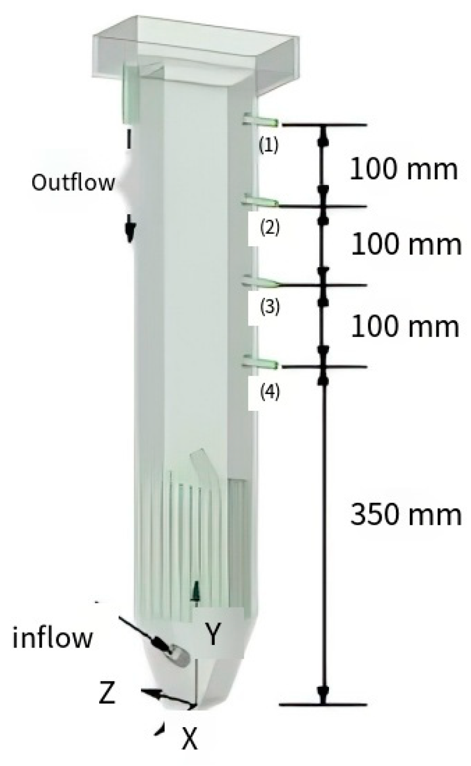
2. Experimental System and the Detection Principle

2.1. Experimental Equipment

Description of the Experimental System

As shown in Figure 1. The experimental system for concentration detection based on interference rectification consists of a circulating pulp tank, slurry pump, valves, defoamer, flow meter, turbulence dissipation measuring tank, and signal acquisition system. The defoamer primarily eliminates bubbles generated during slurry mixing in the circulating slurry tank and slurry pump under pressure, reducing interference during detection as the liquid flows through the pipeline. The turbulence dissipation measuring tank comprises a pressure sensor, an observation tank, and a turbulence dissipation structure. The turbulence dissipation structure is made of transparent plexiglass with the following dimensions: height of 100 mm, wall thickness of 2 mm, and a central square hole measuring 10 mm × 10 mm. This structure is positioned inside the observation tank, which is also constructed from transparent plexiglass.
The observation tank includes an inlet tube with an inner diameter of 20 mm, and the nozzle is positioned at a height of 100 mm. The total height of the observation tank is 600 mm, divided into an upper observation section and a lower feeding section. The feeding section has a trapezoidal shape and shares the same wall thickness as the observation section. The feeding tube is mounted on the sloped side of the trapezoidal section at a 45° angle [16]. The position of the sensor [17] is shown in the figure. The sensor measures pressure values at different positions, which are then used to calculate the average suspension density. The concentration value is subsequently determined using the density-to-concentration conversion relationship as follows:
C w = ( ρ 1 ) ρ m ρ m 1 × 1000
where C w is the suspension concentration, ρ m is the density of solids in suspension, and ρ is the liquid density.

2.2. Experimental Principle and Process

During measurement, the slurry is pumped into the device through the inlet pipe connected to the slurry pump. After passing through the turbulence elimination structure for rectification, sensors on the observation tank’s sidewall record pressure values at different positions. The device employs a dynamic measurement method: as the liquid enters through the inflow pipeline, it exits the observation tank via the lower end of the overflow trough. The collected data are transmitted to the signal acquisition system for further calculations to obtain the final results.

2.3. Experimental Scheme Design

The characteristics of the pulp and the measurement process indicate that as the slurry flows upward in the detection device, particle settling occurs due to its suspension behavior. This leads to concentration variations at different measurement locations, causing measurement inaccuracies [18]. During upward movement, particles in the suspension experience forces in different directions, including inertial force, gravity, buoyancy, and drag force, all of which influence the movement direction and velocity of solid particles [19]. Among these forces, gravity and buoyancy remain unaffected by flow speed, while inertial force depends on particle flow speed, and drag force is influenced by both slurry and particle flow speeds. To maintain measurement accuracy, the inflow speed must be controlled according to the feeding concentration. When the flow velocity of the slurry approaches the particle velocity, the drag force significantly decreases, effectively reducing particle settling, ensuring measurement flow stability, and improving accuracy. Under experimental conditions, although there is a small slip velocity, its effect on drag can be ignored under this optimized flow rate.
This study analyzes the flow field characteristics in the measuring tank under different flow rates and coal slime concentrations to explore how feeding conditions influence measurement accuracy. These findings establish a foundation for precise concentration measurements.
In the experiment, dry coal slime was used to prepare slurry with concentrations of 10% and 30%. The maximum particle size in the slime was 0.5 mm, with an average particle diameter (D) of 0.33 mm and a density of 1.50 g/cm3. Consequently, the slurry densities for the two concentrations were 1.05 and 1.15 g/cm3, respectively. Clean water and these two slurry concentrations were used as experimental samples. Concentration measurements were conducted at inflow velocities of 0.3, 0.4, 0.5, 0.6, 0.7, 0.8, and 0.9 m/s. Five independent tests were conducted for each inflow velocity, with the average value recorded. In each test, after stabilizing the flow rate, all sensor readings over 5 s were collected, and their average was taken as the final result for that test.

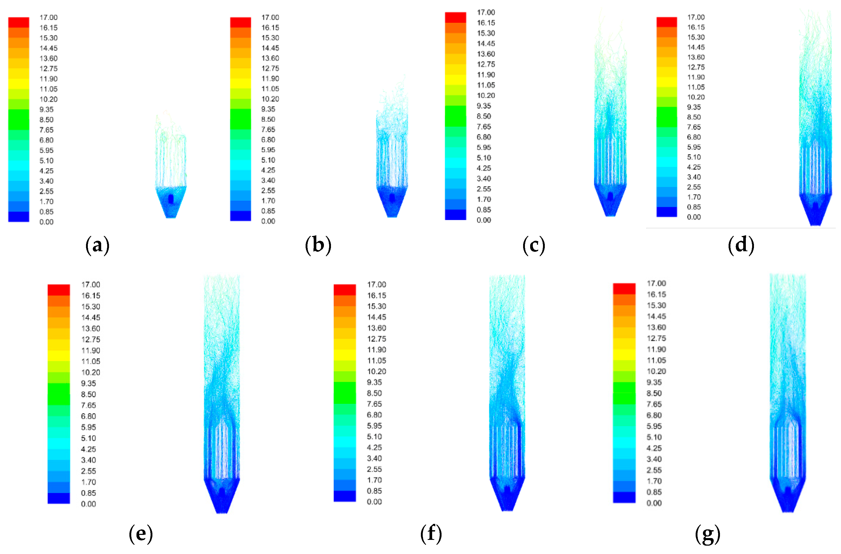
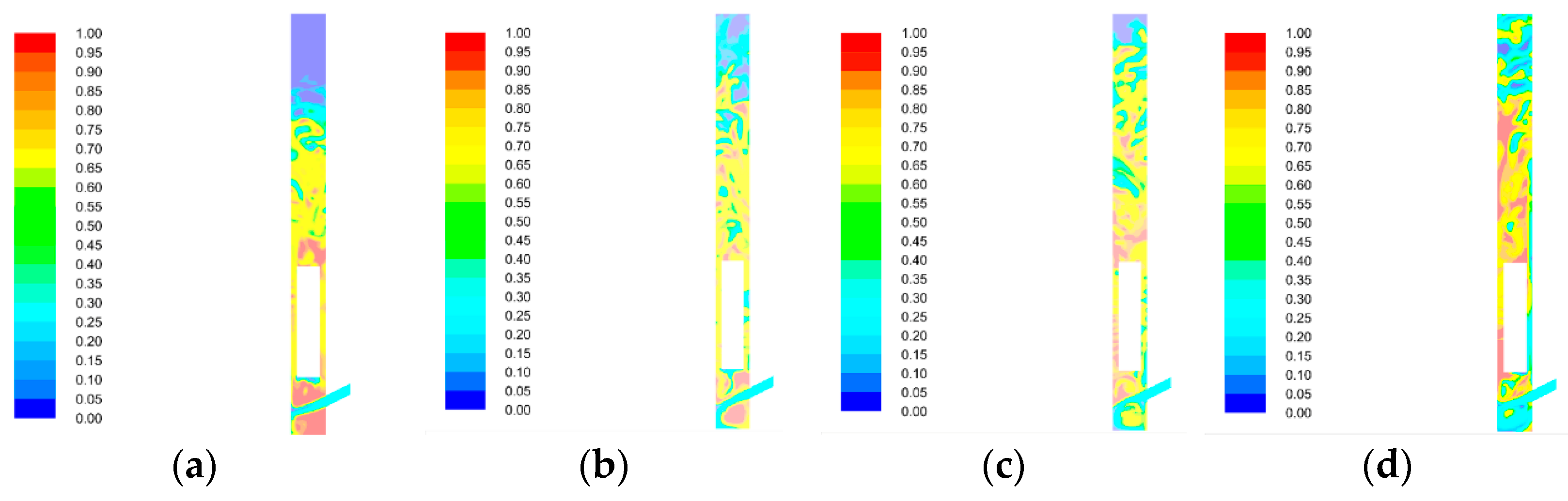
3. Numerical Simulation

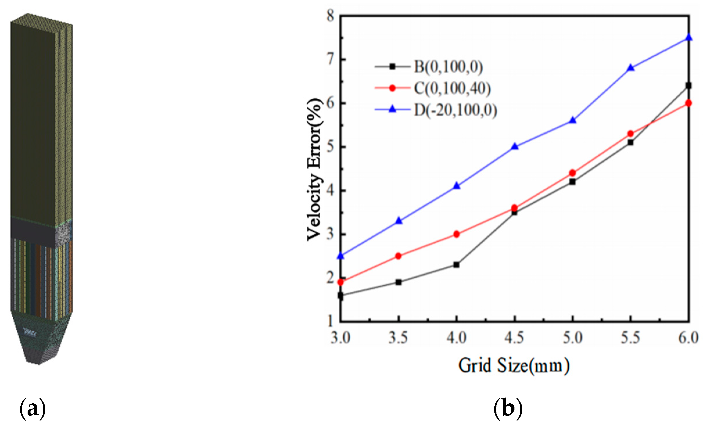
3.1. Establishing Turbulence Dissipation Measurement Tank Model

Figure 2 illustrates the structure of the turbulence elimination measurement tank. The coordinate origin is defined at point A, located at the center of the bottom nozzle. The vertical direction is set as the positive Y axis, while the trapezoidal surface perpendicular to the feeding section is set as the positive X axis. Similarly, the narrow surface perpendicular to the observation section is set as the positive Z axis.

3.2. Numerical Model Settings

To develop the three-dimensional model of the turbulence dissipation measurement tank, the internal flow field is divided into grids using the grid module. Structural grids are applied to the observation tank and turbulence elimination structure, while the remaining parts use nonstructural tetrahedral grids. Once meshing is complete, the results are imported into the Fluent software. Solid–liquid two-phase flow is simulated numerically by treating solid particles as either a quasi-fluid or a discrete phase. The two commonly used models for this are the Euler–Euler model and the Euler–Lagrange model [20].
For low-concentration particle flows, the Euler–Lagrange model is used in the numerical simulations. Specifically, the discrete phase model (DPM) in the Fluent software simulates the trajectory of solid particles, with the flow field characteristics represented by particle trajectories [21]. A particle flow with a density of 1.05 g/cm3 is considered a low-concentration slurry flow, where solid particles constitute 10% of the total volume. The simulation process consists of two steps. First, the continuous flow field is computed until it stabilizes. Once stability is achieved, the DPM model is applied to display the particle trajectory from the inlet. The continuous flow field settings remain unchanged, with the turbulence model set to the standard k-epsilon model. The k-epsilon model has high computational efficiency in solving fully developed turbulence and high compatibility with complex internal flows in storage tanks. By simultaneously solving the transport equations of turbulent kinetic energy (k) and dissipation rate (ε), the model achieves a balance between accuracy and efficiency. At the same time, the stable solution enhanced by wall functions captures critical turbulence characteristics. The semi-implicit method for the pressure-linked equations consistent (SIMPLEC) model is employed for pressure–velocity coupling. The pressure gradient and momentum gradient are discretized using a second-order upwind scheme, while the turbulent kinetic energy and dissipation rates are discretized using a first-order upwind scheme. After the continuous flow field stabilizes, the DPM model is activated for interaction with the continuous phase, and a jet source is created. The experimental material used was carbon-s, with a density of 1.50 g/cm3.
For high-concentration particle flows, the Euler–Euler model is used to simulate the mutual diffusion of the solid–liquid phases, with flow field characteristics described by phase distribution. A particle flow with a density of 1.15 g/cm3 is considered a high-concentration slurry flow, where solid particles make up 30% of the total volume. In this case, a two-phase flow model is applied. The system settings for the flow field remain consistent with the previous simulation using the standard k-epsilon turbulence model. The SIMPLEC model is employed for pressure–velocity coupling. The pressure and momentum gradients are approximated using a second-order upwind scheme, while the turbulent kinetic energy and dissipation rates are discretized using a first-order upwind scheme. The inflow material consists of two phases: liquid (phase 1) and carbon-solid (phase 2). The inlet boundary condition is defined as a velocity inlet with a flow temperature of T = 20 °C, corresponding to a kinematic viscosity of ν = 1.00381 × 10⁻³ m2/s and an inlet turbulence intensity of 5%. The outlet boundary condition is set as outflow. For the solid walls, the standard wall function is applied, incorporating a no-slip shear condition.
The continuous phase governing equations are based on the mass conservation and momentum conservation laws. The mass conservation equation (continuity equation) is as follows:
ρ t + ( ρ u ) x + ( ρ v ) y + ( ρ w ) z = 0
where ρ represents fluid density, t is time, and u , v , and w are the components of the velocity vector in different directions.
The momentum conservation equation is a representation of the momentum conservation law, which mainly refers to the rate of change of the momentum of the fluid in a microelement over time being equal to the sum of the various forces acting on the microelement from the outside. The momentum equations in the three directions on the spatial coordinate system are as follows:
( ρ u ) t + d i v ( ρ u U ) = p x + τ x x x + τ y x y + τ z x z + F x
( ρ v ) t + d i v ( ρ v U ) = p y + τ x y x + τ y y y + τ z y z + F y
( ρ w ) t + d i v ( ρ u U ) = p x + τ x z x + τ y z y + τ z z z + F z
where p is the pressure on the element, τ x x , τ y y , and τ z z are the components of the viscous stress τ on the surface of the microelements, and F x , F y , and F z represent the vertical z-axis of physical force on the element.
The k-epsilon turbulence model used in this study has its turbulent flow energy k and turbulent flow energy dissipation rate ε determined by the following equation:
t ( k ρ ) + x j ( ρ k u j ) = x j [ ( u + u t σ k ) k x j ] + p k ρ ε
t ( k ε ) + x j ( ρ ε u j ) = x j [ ( u + u t σ ε ) ε x j ] + ε k ( C 1 p k C 2 ρ ε )
where p k = u t u i x i ( u i x j + u i x i ) , and the values of k and ε determine that u t = c u ρ k 2 / ε .
Three coordinate points, namely (0, 100, 0), (0, 100, 40), and (−20, 100, 0), were selected in both models to analyze the inflow velocity under different mesh densities [22]. As shown in Figure 3, the velocity errors at these three points, obtained through numerical calculations, gradually decrease as the mesh size is refined. For example, when the mesh size is 4.5 mm, the velocity error at all three positions is less than 5%. When the mesh size is reduced to 3.0 mm, the maximum velocity error is 2.5%, and the simulated velocity values converge, indicating that further mesh refinement does not affect the simulation results. In this study, the cell mesh [23].

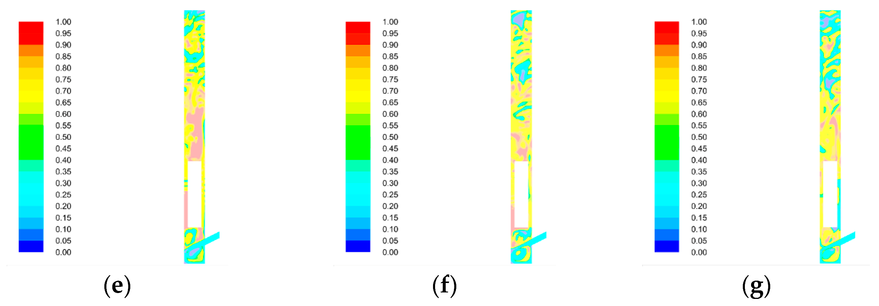
4. Numerical Simulation

Influence of Particle Content on Detecting the Flow Field

Figure 4 shows the particle trajectory diagram at the X = 0 m section in the flow field of the measurement channel at different flow rates when a low particle flow concentration is intercepted.
Figure 4 illustrates the trajectory distribution of particles in a low-density particle flow within the detection device. Based on the observed distribution trends, when the inflow velocity is low, particle dispersion is minimal, with particles primarily concentrated in the inflow section and exhibiting localized diffusion into the flow channel’s turbulent structure. As the inflow velocity increases, particles move upward along the observation tank with the fluid and spread radially inside the tank. At an inflow velocity of 0.6 m/s, particle diffusion extends throughout the device, though uniform suspension is not yet achieved. When the velocity reaches or exceeds 0.7 m/s, the upper end of the turbulence elimination structure becomes evenly distributed. To ensure stable slurry concentration measurements, it is essential to fill the entire device with slurry, which requires maintaining an inflow velocity of ≥0.7 m/s.
For high-concentration particle flows, the phase distribution diagram for the X = 0 m section in the flow field in the gutter at different flow rates is shown in Figure 5 below.
Figure 5 shows the phase distribution of the liquid phase in the suspension with high particle flow concentrations at different inflow velocities. For such high-concentration suspensions, the liquid phase distribution trends reveal that when the inflow velocity is small, the liquid phase is mainly concentrated at the edges of the inlet and outlet of the turbulence elimination structure. This observation indicates an uneven liquid–solid phase distribution within the detection device. With the increase in the inflow velocity, the liquid phase gradually diffuses toward the upper part of the observation tank. At an inflow velocity of 0.8 m/s, the distribution of the solid–liquid phases becomes relatively uniform across the observation tank, eliminating large single-phase concentration areas. Therefore, when the high-concentration pulp is stably measured, it is critical to ensure even filling of the observation and measurement tank by maintaining an inflow velocity ≥0.8 m/s.

5. Analysis of the Experimental Results

5.1. Research on the Measurement Accuracy of the Detection Device Under Different Pulp Concentrations

To further analyze the influence of inflow characteristics on the sensor’s measurement stability, an error analysis was conducted on the test results at different pulp concentrations (1.00, 1.05, and 1.15 g/cm3) and inflow velocities (0.3–0.9 m/s). The error calculation method is as follows:
η = | Δ p i Δ p Δ p | × 100 %
where η represents the error between the measured and calculated pressure differences, Δ p i denotes the measured pressure difference, and Δ p represents the calculated pressure difference.

5.2. Research on the Measurement Accuracy of Particle Flow to the Detection Device

The distance between sensor No. 1 and sensor No. 3 is 20 cm, with the measured pressure difference denoted as ΔP1. Similarly, the distance between sensor No. 2 and sensor No. 4 is also 20 cm, with the measured pressure difference represented as ΔP2. The pressure difference measurements for pulp at different concentrations and inflow velocities are shown in Table 1, Table 2 and Table 3.
The error analysis results are as follows. Figure 6 presents the error distribution of the measurement results. The error analysis reveals that ΔP1 (from sensors No. 1 and No. 3) has a higher error than ΔP2 (from sensors No. 2 and No. 4), indicating that the measurement accuracy of sensors No. 2 and No. 4 is superior. As pulp concentration increases, measurement error No. 2 and No. 1 gradually decreases, with fluctuations remaining within a reasonable range of 1%.
Inflow velocity considerably affects measurement accuracy. At low inflow velocities, measurement error is higher; for example, at 0.3 m/s, the error is 1.07%. As the inflow velocity increases, the measurement error decreases, reaching 0.84% at 0.7 m/s, improving measurement stability. This improvement is primarily due to higher velocity-reducing sedimentation effects, promoting uniform material mixing, and leading to a more homogeneous pulp distribution consistent with the numerical simulation results. However, when the inflow velocity reaches 0.9 m/s, the measurement error increases, and stability declines. This instability is attributed to flow disturbances in the upper part of the measurement tank and increased dynamic pressure, both of which contribute to higher measurement error.

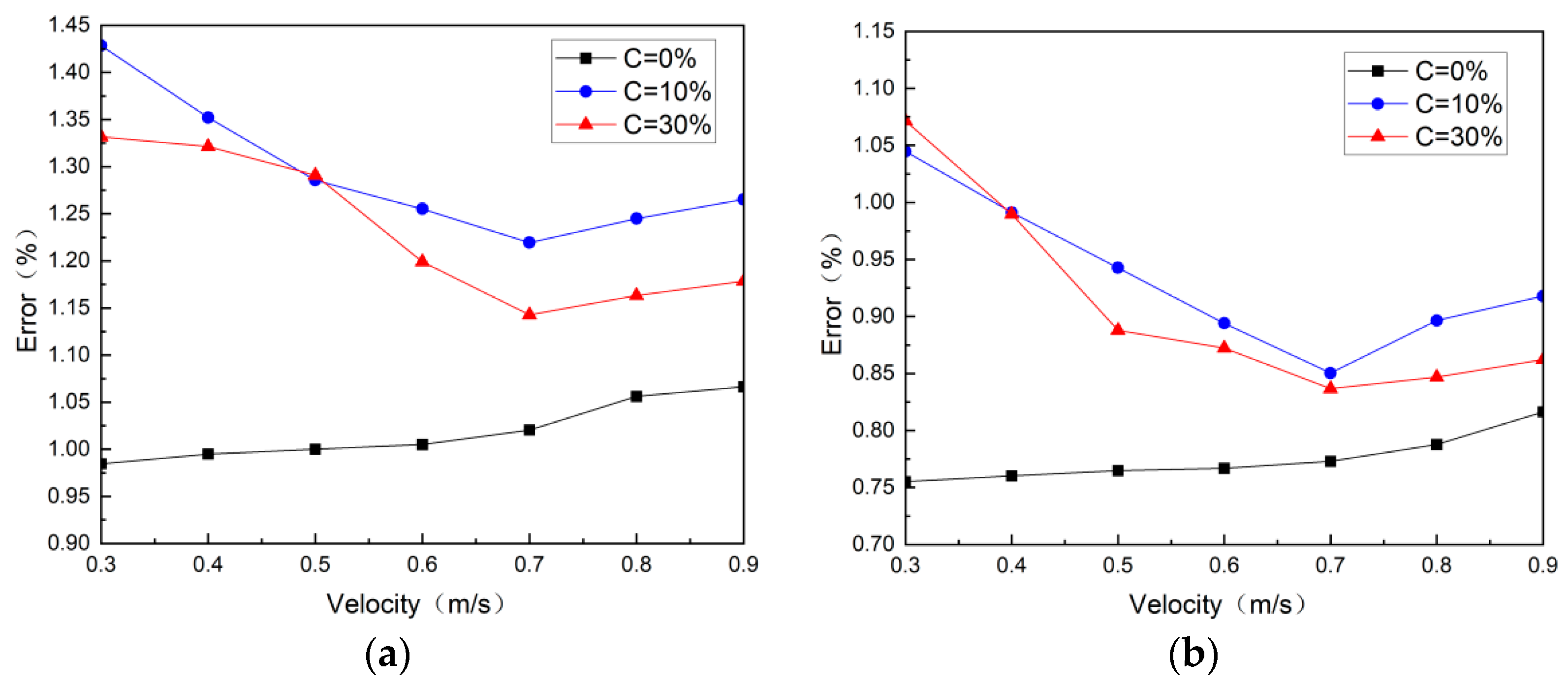
5.3. Error Analysis and Discussion of Discrepancies

The experimental and numerical results collectively demonstrate a nonlinear coupling between detection errors and the synergistic effects of flow velocity and slurry concentration. Systematic comparisons reveal that sensor pair No. 2–4 exhibits significantly lower measurement errors than sensor pair No. 1–3, as evidenced by the ΔP2 error stabilizing below 0.84% for low-concentration slurries at the critical velocity of 0.7 m/s. Numerical simulations corroborate this observation, showing reduced turbulent kinetic energy and enhanced particle uniformity in central flow regions, which aligns with the optimized positioning of the sensors in hydrodynamic stability zones. By contrast, elevated errors for sensor pair No. 1–3 at subcritical velocities stem from gravitational sedimentation-induced concentration gradients, validated by both experimental pressure fluctuations and simulated particle aggregation patterns.
Increasing flow velocity beyond 0.7 m/s enhances kinetic energy and stabilizes particle dispersion. However, surpassing 0.8 m/s triggers turbulence resurgence in the upper measurement channel, with the Reynolds number exceeding Re = 2300, marking the transition to turbulent flow. This amplifies dynamic pressure perturbations and explains the nonlinear error rebound observed experimentally. High-concentration slurries exhibit reduced error variability compared to low-concentration systems, as elevated solid-phase interactions suppress turbulence and improve homogeneity. Achieving stability for high-concentration slurries necessitates higher critical velocities, emphasizing the regulatory role of concentration–velocity synergy in hydrodynamic thresholds.
Potential systematic errors include residual microbubbles from incomplete defoaming, unresolved microscale vortices due to mesh resolution limitations, and trajectory biases from spherical particle assumptions. These factors contribute to deviations at extreme velocities, underscoring the need for refined particle morphology modeling and boundary-layer turbulence resolution to enhance predictive accuracy under non-ideal conditions.

6. Conclusions

(1)
The combined fluid simulation and the experimental results confirm that inflow characteristics notably influence the accuracy of pulp concentration measurements. By integrating CFD modeling with a novel interference rectification structure, this study systematically reveals the nonlinear coupling mechanism between flow velocity and turbulence suppression. Numerical simulations indicate that as inflow velocity increases, turbulence in the observation measurement tank decreases, leading to greater particle dispersion and a more uniform distribution. The experimental results further demonstrate that increased inflow velocity enhances dispersion uniformity, thereby reducing measurement error. However, further increases in the flow rates reduce flow field stability and increase dynamic pressure, resulting in higher measurement errors.
(2)
The numerical simulations demonstrate that achieving a uniform suspension of solid particles in high-concentration slurries (C = 30%) requires significantly greater inflow velocities (≥0.8 m/s) compared to low-concentration systems. The optimized sensor configuration (No. 2 and No. 4) minimizes boundary turbulence interference by leveraging flow field stability in central regions. The experimental results confirm that higher concentrations lead to lower measurement errors, while fluctuations remain within a reasonable range of approximately 1%.

Author Contributions

Conceptualization, C.W. and P.S.; methodology, C.W.; software, Z.L.; validation, D.Y.; formal analysis, C.W.; investigation, P.S.; resources, C.W.; data curation, P.S.; writing—original draft preparation, P.S.; writing—review and editing, C.W.; visualization, P.S.; supervision, C.W. All authors have read and agreed to the published version of the manuscript.

Funding

This research received no external funding.

Data Availability Statement

The original contributions presented in this study are included in the article. Further inquiries can be directed to the corresponding authors.

Conflicts of Interest

The authors declare no conflicts of interest.

References

  1. Zhao, Y.; Meng, L.; Shen, X. Study on ultrasonic-electrochemical treatment for difficult-to-settle slime water. Ultrason. Sonochemistry 2020, 64, 104978. [Google Scholar] [CrossRef]
  2. Ding, S.; Pan, F.; Zhou, S.; Bu, X.; Alheshibri, M. Ultrasonic-assisted flocculation and sedimentation of coal slime water using the Taguchi method. Energy Sources Part A Recovery Util. Environ. Eff. 2023, 45, 10523–10536. [Google Scholar] [CrossRef]
  3. M, E.V.; M, S.O.; T, M.A. Study of concentrating plants’ coal slurry dewatering. J. Min. Geotech. Eng. 2024, 24. [Google Scholar]
  4. Муркo, Е.В.; Маркoв, С.О. Тюленев, М.А. ИССЛЕДОВАНИЕ ОБЕЗВОЖИВАНИЯ УГОЛЬНОГО ШЛАМА ОБОГАТИТЕЛЬНЫХ ФАБРИК. ТЕХНИКА 2024, 1, 58–76. [Google Scholar]
  5. Wu, W.-J.; Zheng, Q.-J.; Liang, J.-W.; Zhao, H.-M.; Liu, B.-L.; Li, Y.-W.; Feng, N.-X.; Cai, Q.-Y.; Xiang, L.; Mo, C.-H.; et al. Mining flotation reagents: Quantitative and robust analysis of metal-xanthate complexes in water. J. Hazard. Mater. 2024, 476, 134873. [Google Scholar] [CrossRef] [PubMed]
  6. Burdonov, A.E.; Verochkina, E.A.; Rozentsveig, I.B.; Vchislo, N.V. Xanthates and Dithiocarbamates: Synthesis, Characterization and Application in Flotation Processes. Mini-Rev. Org. Chem. 2024, 22, 44–53. [Google Scholar]
  7. Taşdemir, T.; Taşdemir, A. Modeling and optimization of reagent dosages and pH for efficient floc-flotation of suspended particles in Jameson flotation cell by CCD. J. Water Process Eng. 2023, 55, 104243. [Google Scholar] [CrossRef]
  8. Duchnowska, M.; Bakalarz, A.; Luszczkiewicz, A. Influence of reagent dose on the flotation selectivity of copper ore from LGOM area (SW Poland). IOP Conf. Ser. Mater. Sci. Eng. 2019, 641, 012016. [Google Scholar] [CrossRef]
  9. Cao, B.F.; Xie, Y.F.; Yang, C.H.; Gui, W.H.; Li, J.Q. Reagent Dosage Control for the Antimony Flotation Process Based On Froth Size Pdf Tracking and an Index Predictive Model. J. Min. Sci. 2020, 55, 452–468. [Google Scholar] [CrossRef]
  10. Sun, B.; Chen, S.; Liu, Q.; Lu, Y. Review of sewage flow measuring instruments. Ain Shams Eng. J. 2020, 12, 2089–2098. [Google Scholar] [CrossRef]
  11. Li, Y.; Peng, S.; Song, Z.; Wang, F. Measurement of two phase flow concentration with a novel pressure difference method. I: Principle. Flow Meas. Instrum. 2024, 97, 102591. [Google Scholar] [CrossRef]
  12. Li, X.; Li, H.; Zhang, J.; Zhou, F.; Chen, A. Measurement of the phosphorite ore pulp density based on the image recognition method. Int. J. Min. Miner. Eng. 2022, 13, 64–75. [Google Scholar] [CrossRef]
  13. de Aquino, G.S.; Martins, R.S.; Martins, M.F.; Ramos, R. An Overview of Computational Fluid Dynamics as a Tool to Support Ultrasonic Flow Measurements. Metrology 2025, 5, 11. [Google Scholar] [CrossRef]
  14. Tan, Y.; Ni, Y.; Xu, W.; Xie, Y.; Li, L.; Tan, D. Key technologies and development trends of the soft abrasive flow finishing method. J. Zhejiang Univ.-Sci. A 2023, 24, 1043–1064. [Google Scholar] [CrossRef]
  15. Tang, H.; Fan, Y.; Ma, X.; Dong, X.; Chang, M.; Li, N. Modelling Flocculation in a Thickener Feedwell Using a Coupled Computational Fluid Dynamics–Population Balance Model. Minerals 2023, 13, 309. [Google Scholar] [CrossRef]
  16. De Castro, B.; Benzaazoua, M.; Chopard, A.; Plante, B. Automated mineralogical characterization using optical microscopy: Review and recommendations. Miner. Eng. 2022, 189, 107896. [Google Scholar] [CrossRef]
  17. Nguyen, T.H.; Tang, F.H.; Maggi, F. Optical Measurement of Cell Colonization Patterns on Individual Suspended Sediment Aggregates. J. Geophys. Res. Earth Surf. 2017, 122, 1794–1807. [Google Scholar] [CrossRef]
  18. Zhang, X.R.; Zhu, Y.G.; Zheng, G.B.; Han, L.; McFadzean, B.; Qian, Z.B.; Piao, Y.C.; O'Connor, C. An investigation into the selective separation and adsorption mechanism of a macromolecular depressant in the galena-chalcopyrite system. Miner. Eng. 2019, 134, 291–299. [Google Scholar] [CrossRef]
  19. Fu, L.; Bai, H.; Bai, D.; Xu, G. Hydrodynamics of gas-solid fluidization at ultra-high temperatures. Powder Technol. 2022, 406, 117552. [Google Scholar] [CrossRef]
  20. Dontsov, E.V. A model for proppant dynamics in a perforated wellbore. Int. J. Multiph. Flow 2023, 167, 104552. [Google Scholar] [CrossRef]
  21. Zhou, H.; Guo, J.; Zhang, T.; Li, M.; Tang, T.; Gou, H. Eulerian multifluid simulations of proppant transport with different sizes. Phys. Fluids 2023, 35, 043314. [Google Scholar]
  22. Liu, H.; Li, Z.; Wang, C.; Zhang, Q. Impacts of inflow conditions on the measurement stability of a turbulence-mitigation based liquid concentration detection system. Flow Meas. Instrum. 2023, 90, 102337. [Google Scholar] [CrossRef]
  23. Kawakita, R.; Strobel, S.; Soares, B.; Scher, H.B.; Becker, T.; Dale, D.; Jeoh, T. Fluidized bed spray-coating of enzyme in a cross-linked alginate matrix shell (CLAMshell). Powder Technol. 2021, 386, 372–381. [Google Scholar] [CrossRef]
Figure 1. Pressure differential concentration detection device and experimental system: (a) pressure differential concentration detection device; (b) differential pressure concentration detection system.
Processes 13 01421 g001
Figure 2. Turbulence elimination measurement tank model.
Processes 13 01421 g002
Figure 3. Simulation analysis diagram: (a) calculation model grid division diagram; (b) velocity error diagram.
Processes 13 01421 g003
Figure 4. Particle distribution at different inlet velocities: (a) V = 0.3 m/s; (b) V = 0.4 m/s; (c) V = 0.5 m/s; (d) V = 0.6 m/s; (e) V = 0.7 m/s; (f) V = 0.8 m/s; (g) V = 0.9 m/s.
Processes 13 01421 g004
Figure 5. Phase distribution at different inlet velocities: (a) V = 0.3 m/s; (b) V = 0.4 m/s; (c) V = 0.5 m/s; (d) V = 0.6 m/s; (e) V = 0.7 m/s; (f) V = 0.8 m/s; (g) V = 0.9 m/s.
Processes 13 01421 g005aProcesses 13 01421 g005b
Figure 6. Measurement error of different concentrations of liquid varies with inflow velocity: (a) ΔP1 error result graph; (b) ΔP2 error result graph.
Processes 13 01421 g006
Table 1. Table of pressure difference measurement results in a clean water medium.
Inflow Velocity (m/s)0.30.40.50.60.70.80.9
ΔP11.9411.9411.9401.9401.9401.9391.939
ΔP21.9451.9451.9451.9451.9451.9451.944
Table 2. Results of pressure difference measurements for 10% concentration liquid.
Inflow Velocity (m/s)0.30.40.50.60.70.80.9
ΔP12.030 2.032 2.033 2.033 2.034 2.034 2.033
ΔP22.037 2.038 2.039 2.040 2.041 2.040 2.039
Table 3. Results of pressure difference measurements for 30% concentration liquid.
Inflow Velocity (m/s)0.30.40.50.60.70.80.9
ΔP12.228 2.228 2.229 2.231 2.232 2.231 2.231
ΔP22.233 2.235 2.237 2.237 2.238 2.237 2.237
Disclaimer/Publisher’s Note: The statements, opinions and data contained in all publications are solely those of the individual author(s) and contributor(s) and not of MDPI and/or the editor(s). MDPI and/or the editor(s) disclaim responsibility for any injury to people or property resulting from any ideas, methods, instructions or products referred to in the content.

