Author Contributions
Conceptualization, T.-H.K., S.-H.B., S.-J.Y., S.-K.L. and J.-W.K.; methodology, T.-H.K., S.-H.B., S.-J.Y., S.-K.L. and J.-W.K.; software, T.-H.K.; validation, T.-H.K., S.-H.B., S.-J.Y., S.-K.L. and J.-W.K.; writing—original draft preparation, T.-H.K.; writing—review and editing, J.-W.K.; supervision, S.-J.Y. and S.-K.L.; project administration, S.-K.L. and J.-W.K. All authors have read and agreed to the published version of the manuscript.
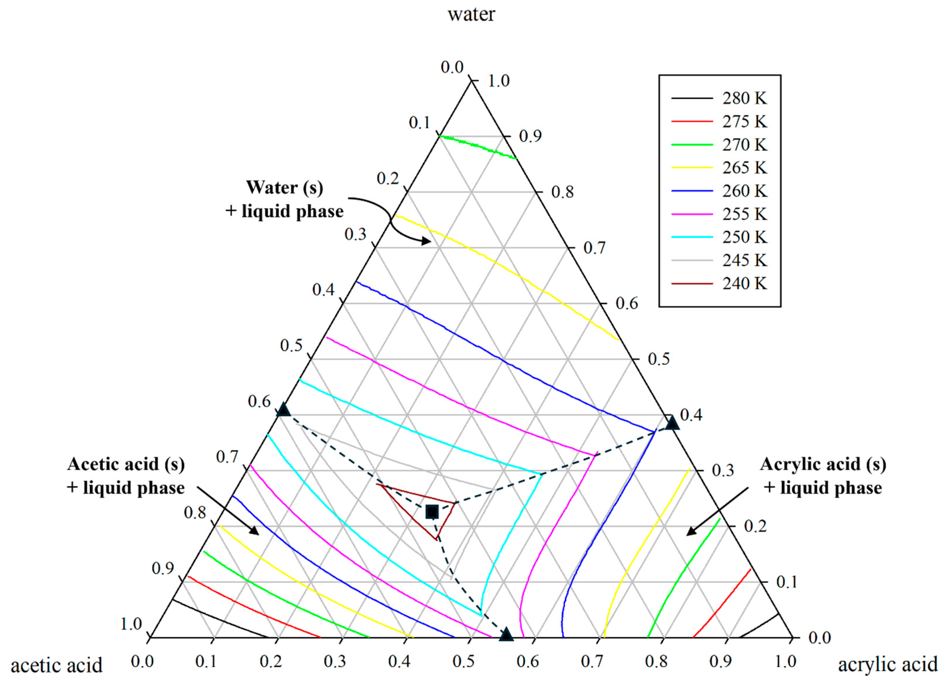
Figure 1.
Ternary solid–liquid equilibrium (SLE) phase diagram for acrylic acid (1) + water (2) + acetic acid (3) system through polythermal projection using UNIQUAC model. The UNIQUAC parameters are derived from our previous study [
11]. Symbols indicate the binary eutectic point (
▲), the ternary eutectic point (
■), and the thermodynamic boundary (--).
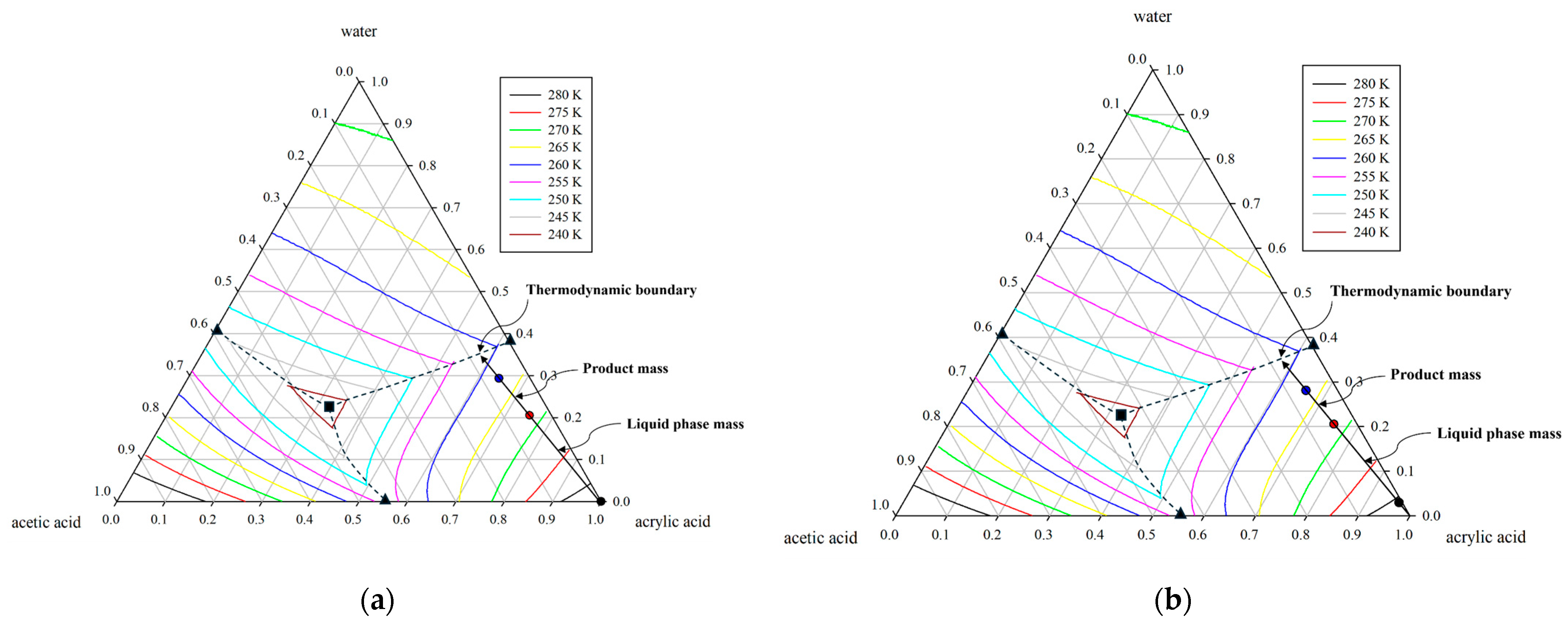
Figure 2.
Ternary solid–liquid equilibrium (SLE) phase diagrams illustrating polythermal trajectories under two distribution coefficient conditions: (a) = 0.0 and (b) = 0.1. The symbols ●, ●, and ● denote the product, feed, and liquid-phase compositions, respectively. The phase diagram also marks the binary eutectic point (▲), the ternary eutectic point (■), and the thermodynamic boundary (--).
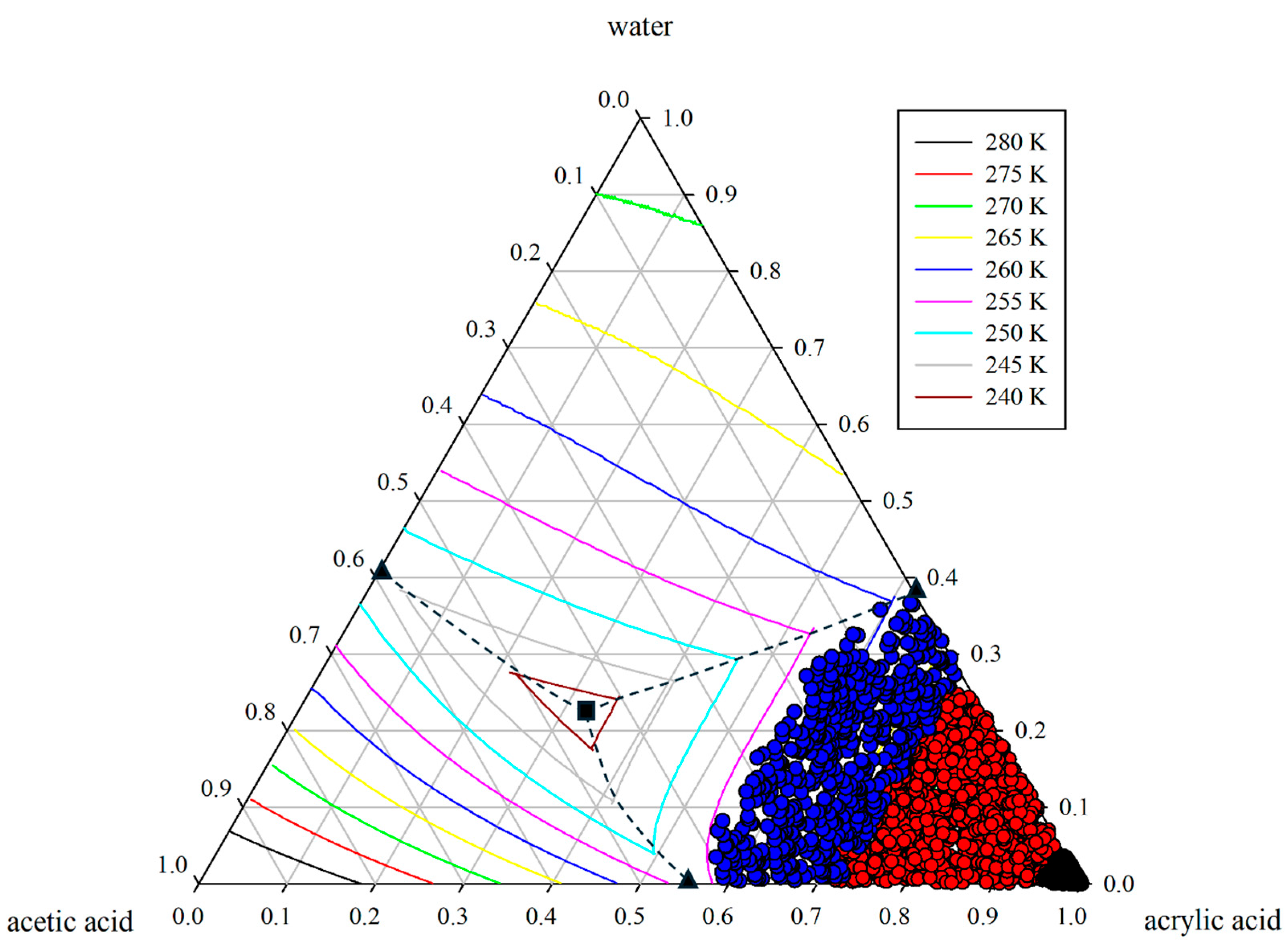
Figure 3.
Ternary solid–liquid equilibrium (SLE) phase diagram illustrating data generation via Latin Hypercube Sampling (LHS). The symbols ●, ●, and ● denote the product, feed, and liquid-phase compositions, respectively. The phase diagram also marks the binary eutectic point (▲), the ternary eutectic point (■), and the thermodynamic boundary (--).
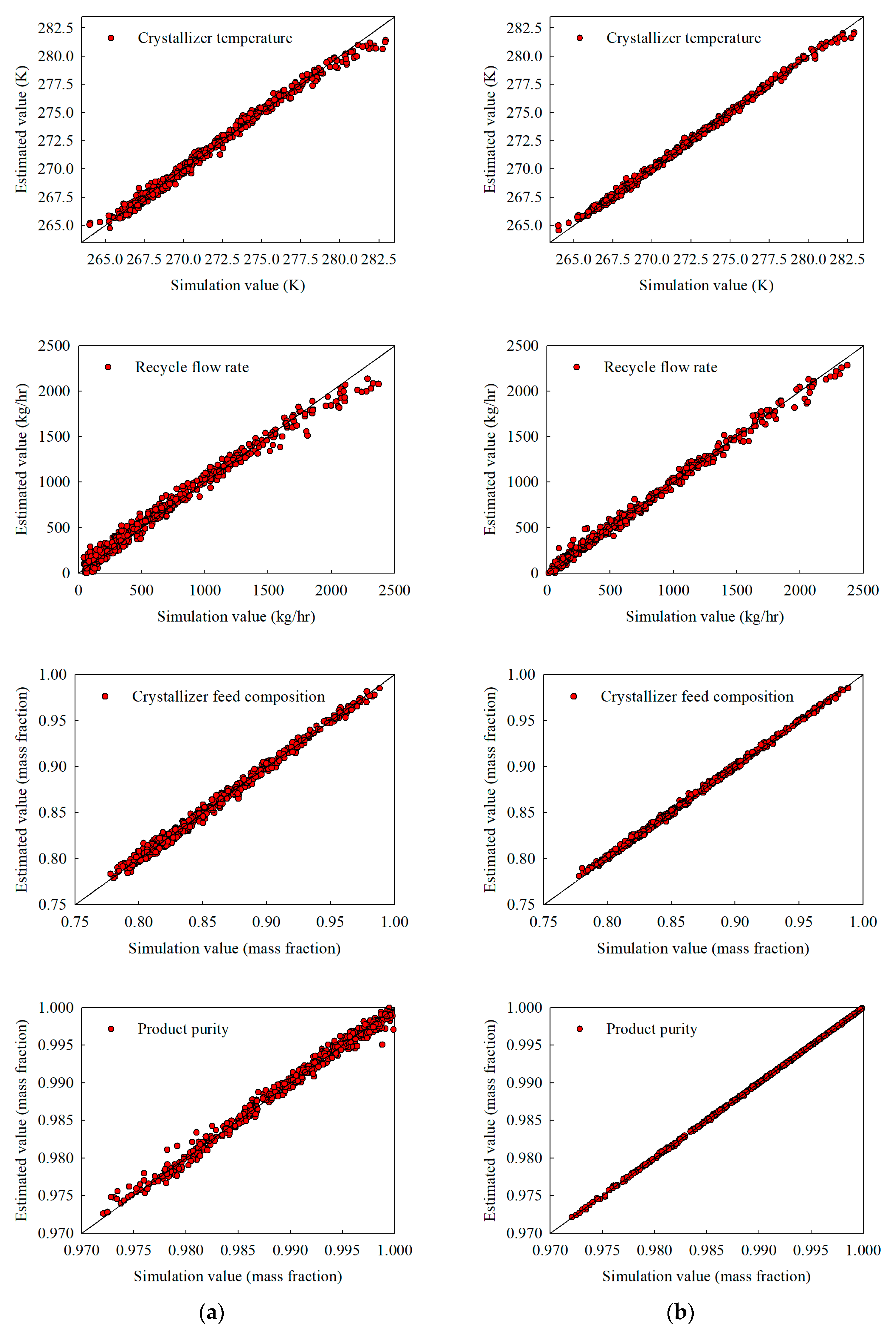
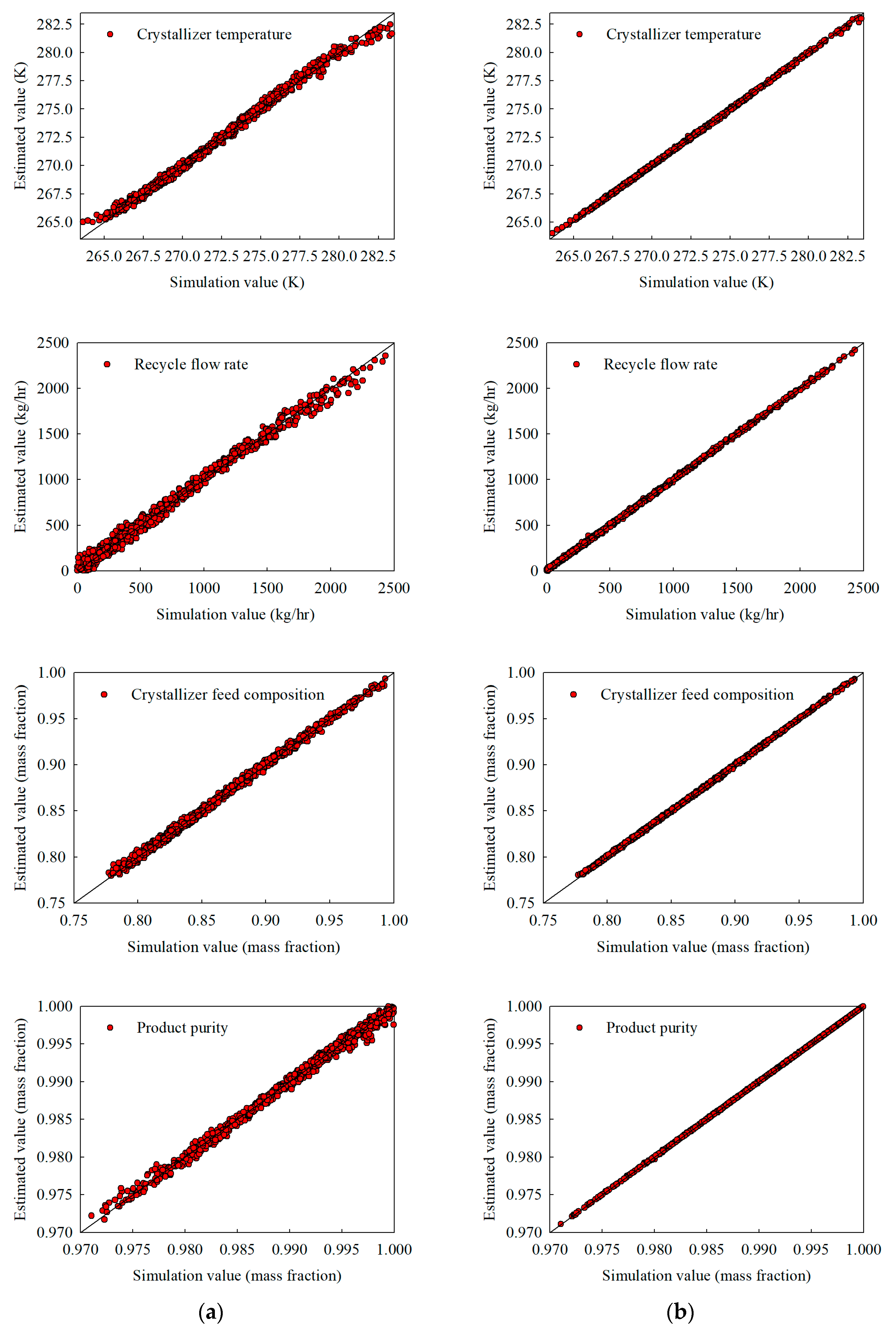
Figure 4.
Interpolation estimates obtained with 500 training samples for (a) the stand-alone NN and (b) the hybrid NN, illustrating crystallizer temperature, recycle flow, crystallizer feed composition, and product purity.
Figure 4.
Interpolation estimates obtained with 500 training samples for (a) the stand-alone NN and (b) the hybrid NN, illustrating crystallizer temperature, recycle flow, crystallizer feed composition, and product purity.
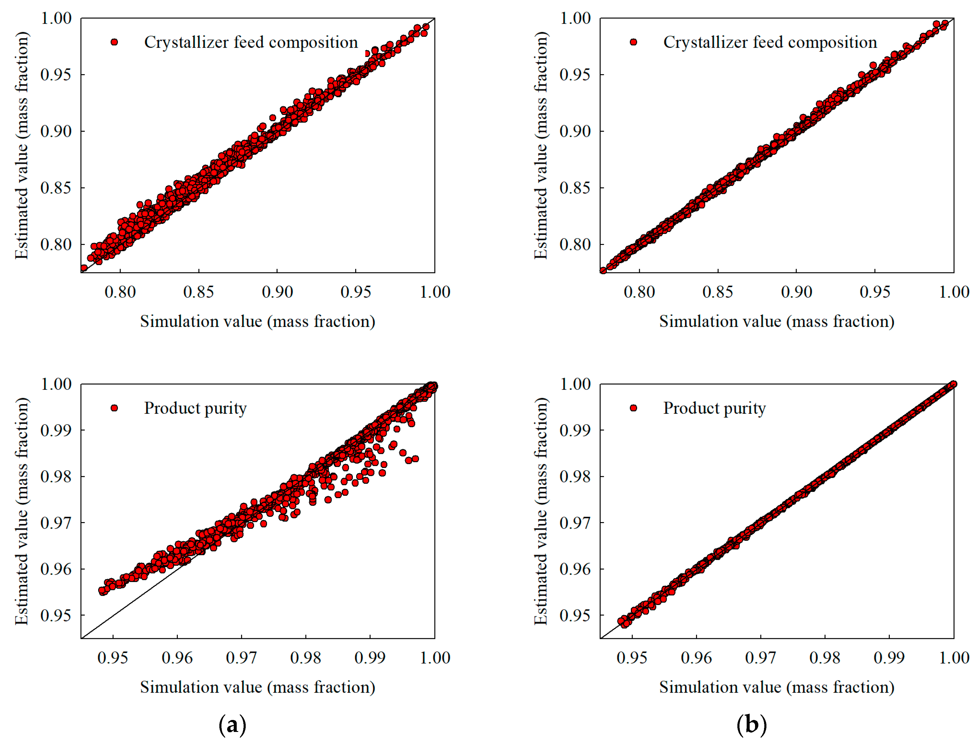
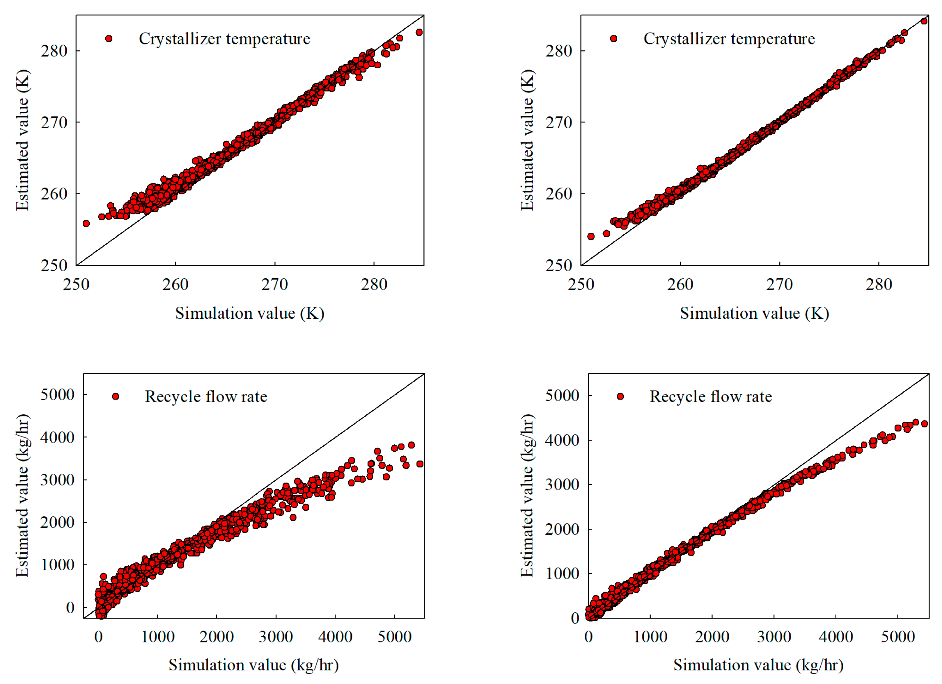
Figure 5.
Interpolation estimates obtained with 3000 training samples for (a) the stand-alone NN and (b) the hybrid NN, illustrating crystallizer temperature, recycle flow, crystallizer feed composition, and product purity.
Figure 5.
Interpolation estimates obtained with 3000 training samples for (a) the stand-alone NN and (b) the hybrid NN, illustrating crystallizer temperature, recycle flow, crystallizer feed composition, and product purity.
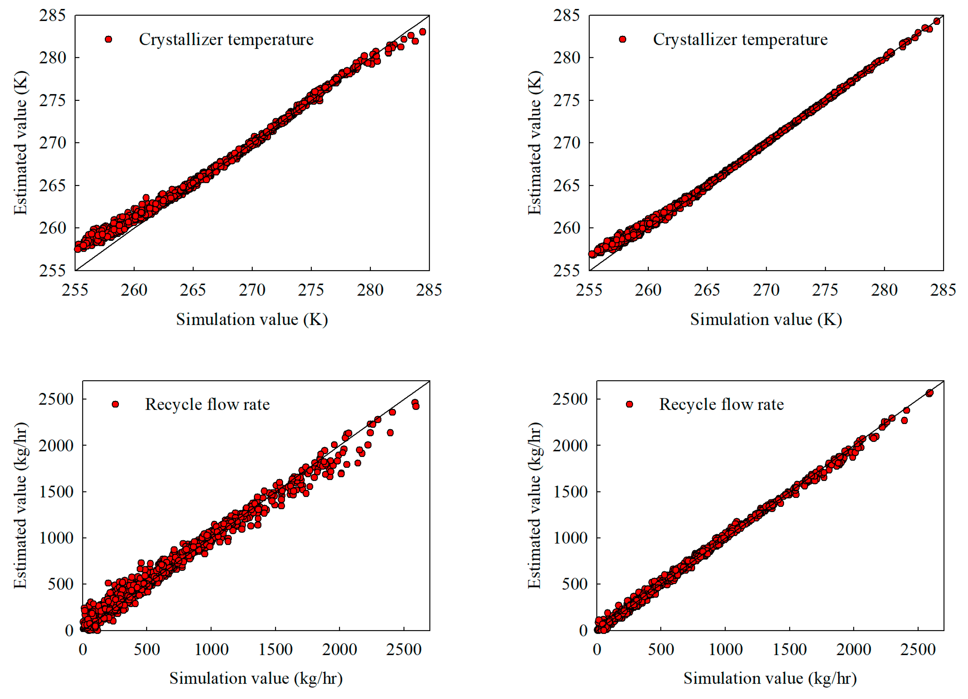
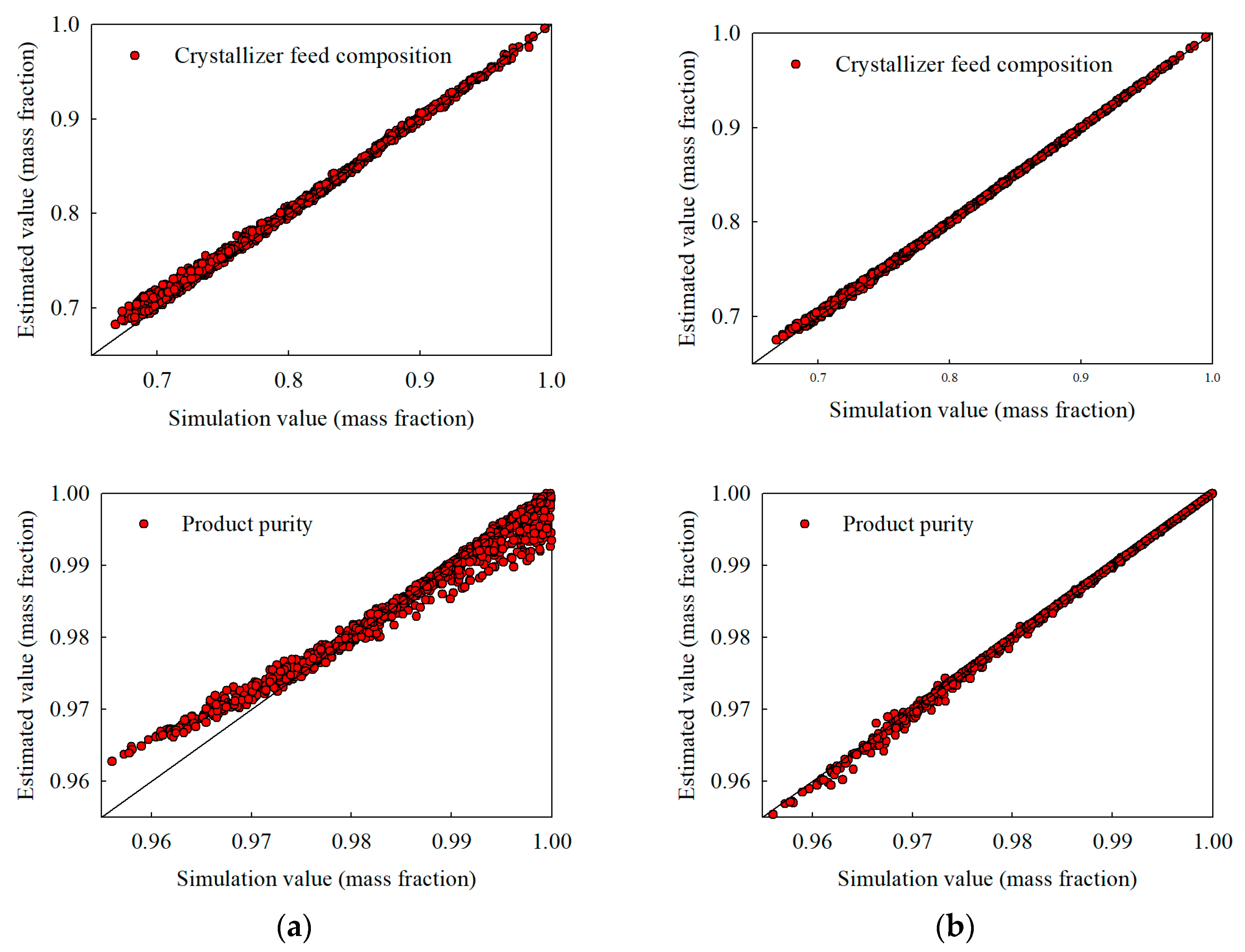
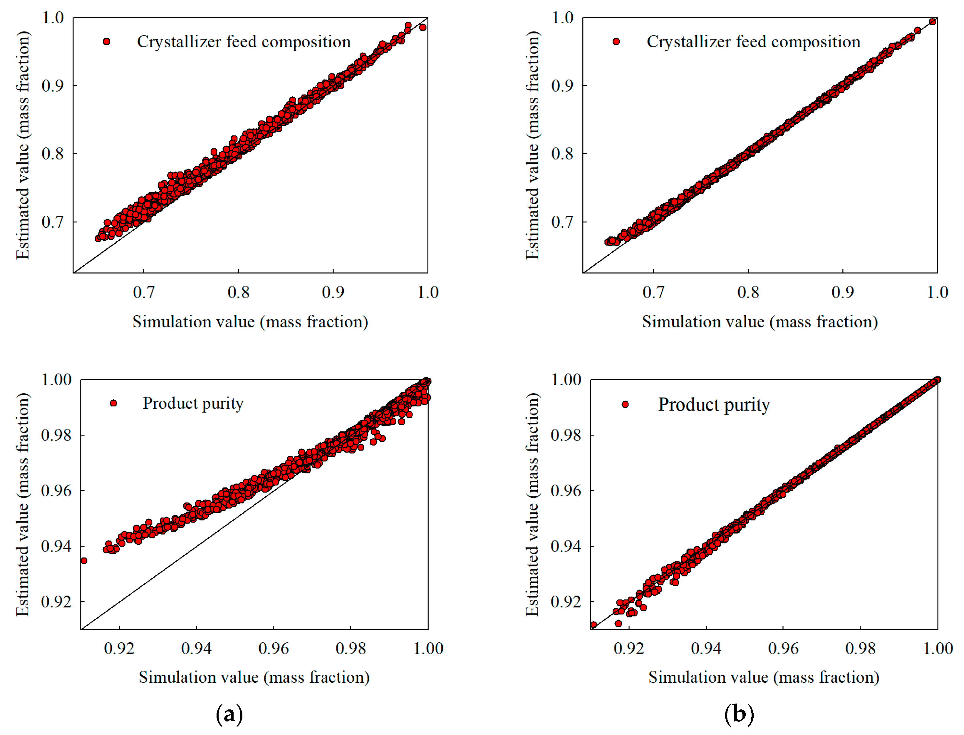
Figure 6.
Extrapolation estimates under a broadened acrylic acid feed composition range of 0.70–1.00 (with water up to 0.25): (a) stand-alone NN and (b) hybrid NN, illustrating crystallizer temperature, recycle flow, crystallizer feed composition, and product purity.
Figure 6.
Extrapolation estimates under a broadened acrylic acid feed composition range of 0.70–1.00 (with water up to 0.25): (a) stand-alone NN and (b) hybrid NN, illustrating crystallizer temperature, recycle flow, crystallizer feed composition, and product purity.
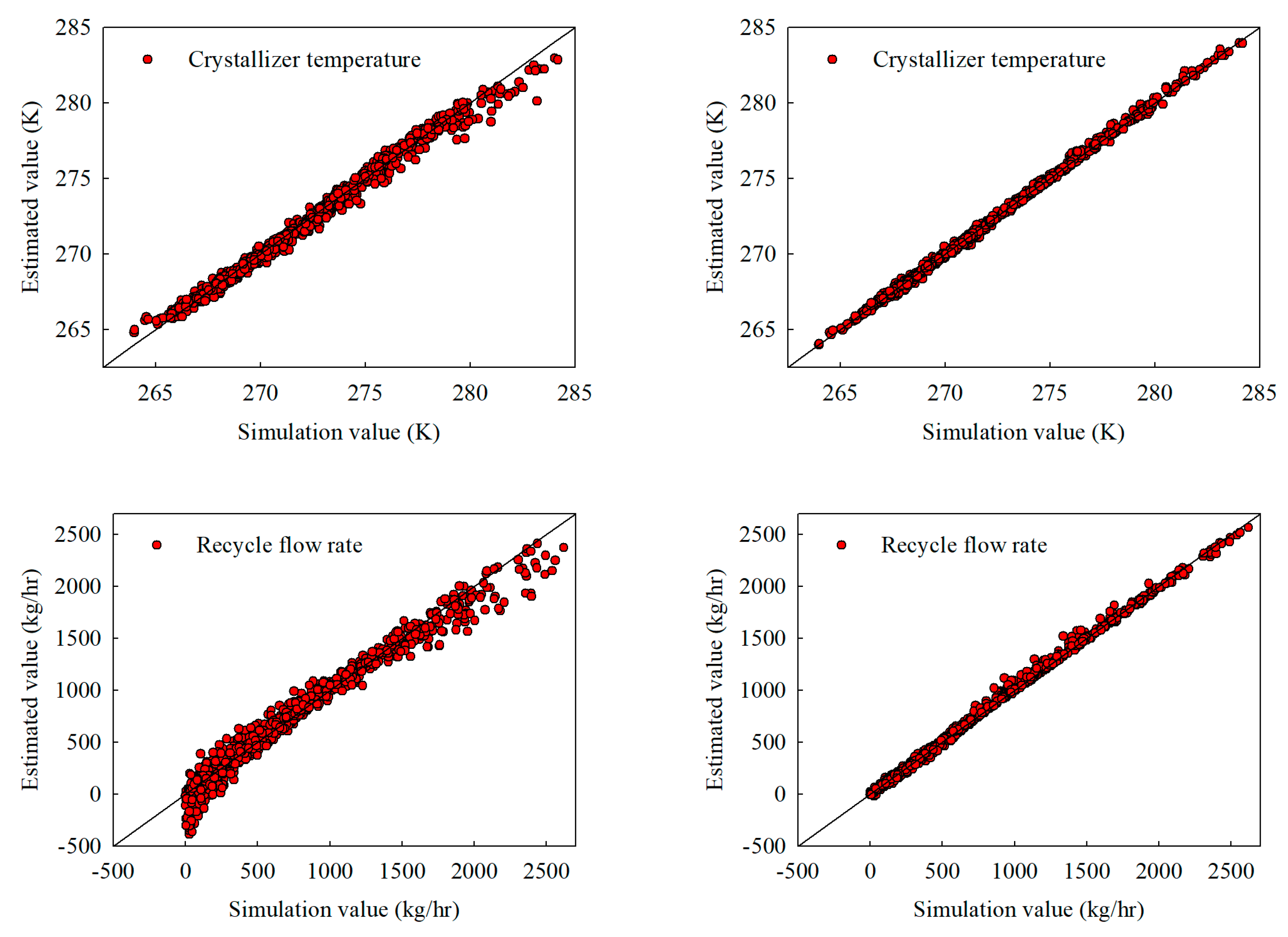
Figure 7.
Extrapolation estimates under a broadened distribution coefficient () range from 0.10 to 0.20: (a) stand-alone NN and (b) hybrid NN, illustrating crystallizer temperature, recycle flow, crystallizer feed composition, and product purity.
Figure 7.
Extrapolation estimates under a broadened distribution coefficient () range from 0.10 to 0.20: (a) stand-alone NN and (b) hybrid NN, illustrating crystallizer temperature, recycle flow, crystallizer feed composition, and product purity.
Figure 8.
Extrapolation estimates under a multi-parameter expansion (acrylic acid composition 0.70–1.00, water 0.00–0.25, feed flow 1000–15,000 kg/h, recycle ratio 0.00–0.40, and 0.00–0.20): (a) stand-alone NN, (b) hybrid NN, illustrating crystallizer temperature, recycle flow, crystallizer feed composition, and product purity.
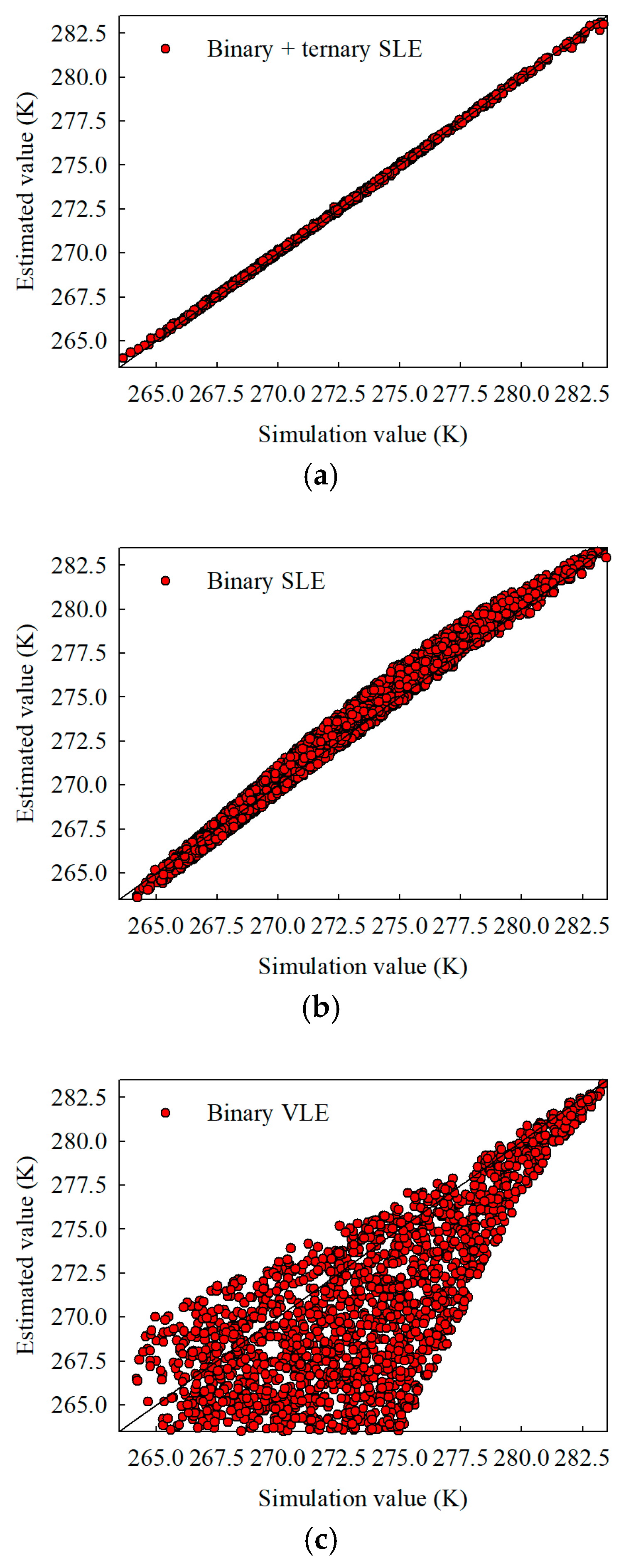
Figure 9.
Interpolation estimates for crystallizer temperature using 3000 training samples under (a) parameter fitted to both binary and ternary solid–liquid equilibrium data, (b) parameters based exclusively on binary solid–liquid equilibrium data, and (c) parameters relying on binary vapor–liquid equilibrium data.
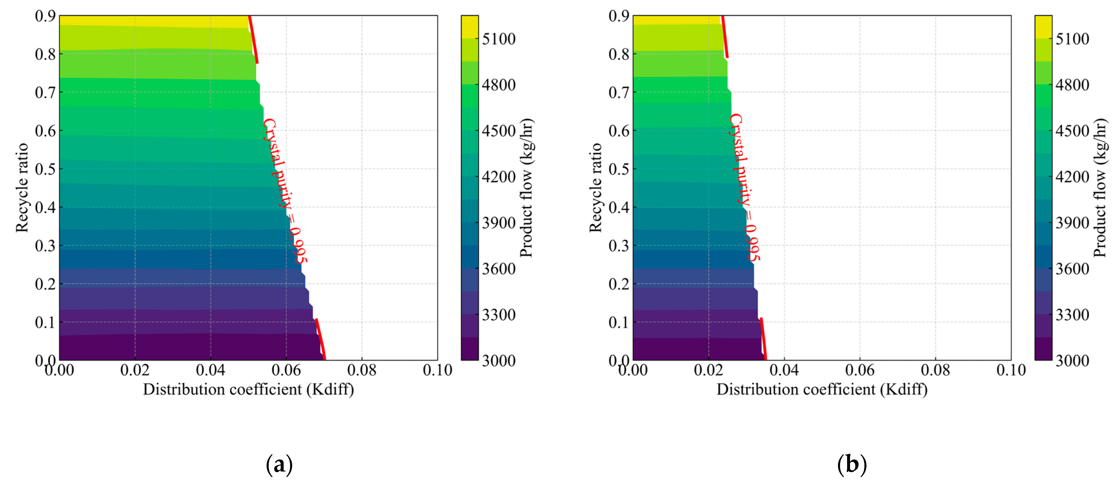
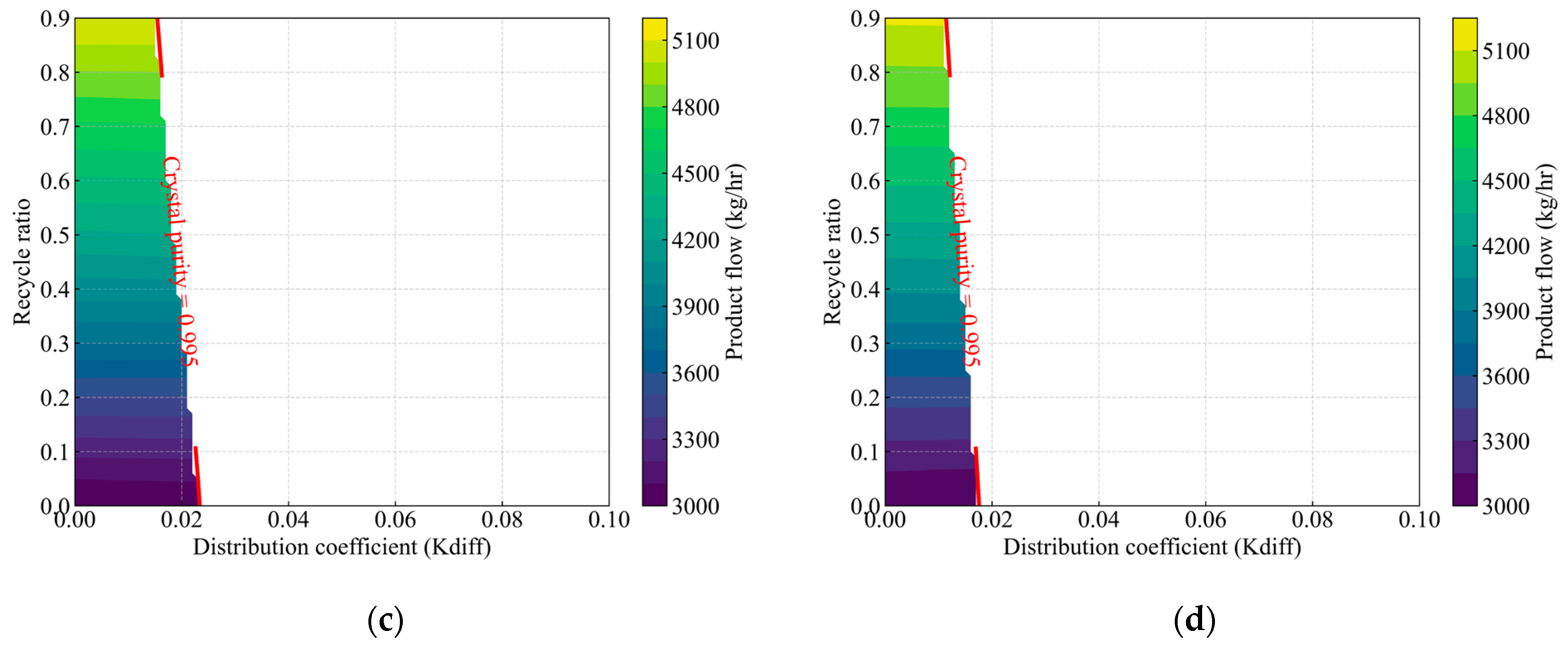
Figure 10.
Effect of the distribution coefficient and recycle ratio on product composition, highlighting the feasible operating region for the crystallization process. The colored contours indicate the product flow rate (kg/h) at each (, recycle ratio) operating condition, while the red-labeled lines (crystal purity = 0.995) represent isopleths defining the boundary at which crystal product purity reaches 0.995. Panels (a), (b), (c), and (d) correspond to feed compositions of acrylic acid at 95 wt%, 90 wt%, 85 wt%, and 80 wt%, respectively.
Table 1.
Parameter ranges considered for sampling and training the neural network models. The target crystal fraction is fixed at 30 wt%.
Table 1.
Parameter ranges considered for sampling and training the neural network models. The target crystal fraction is fixed at 30 wt%.
| Input Variable | Range | Unit |
|---|
| Feed composition | | |
| 0.8–1.0 | mass fraction |
| 0.0–0.16 | mass fraction |
| 0.0–0.04 | mass fraction |
| Feed flow | 1000–10,000 | kg/h |
| 0.0–0.1 | - |
| Recycle ratio (ζ) | 0.0–0.3 | - |
| 30 | % |
Table 2.
Interpolation performance using 500 vs. 3000 training samples for selected output variables. The coefficient of determination () and the root mean squared error (RMSE) are shown for both the stand-alone and hybrid neural network models.
Table 2.
Interpolation performance using 500 vs. 3000 training samples for selected output variables. The coefficient of determination () and the root mean squared error (RMSE) are shown for both the stand-alone and hybrid neural network models.
| Output Variable | 500 Samples | 3000 Samples |
|---|
| (Stand-Alone NN) | (Hybrid NN) | (Stand-Alone NN) | (Hybrid NN) |
|---|
| | R2 | RMSE | R2 | RMSE | R2 | RMSE | R2 | RMSE |
|---|
| Crystallizer temperature | 0.989 | 0.426 | 0.997 | 0.223 | 0.994 | 0.314 | 1.000 | 0.081 |
| Product flow | 0.991 | 83.223 | 0.998 | 42.281 | 0.996 | 52.513 | 1.000 | 11.288 |
| Mother liquor flow | 0.992 | 183.722 | 0.998 | 96.019 | 0.997 | 117.930 | 1.000 | 21.486 |
| Recycle flow | 0.981 | 77.025 | 0.993 | 45.680 | 0.992 | 50.241 | 1.000 | 9.580 |
| Purge flow | 0.992 | 152.073 | 0.998 | 76.544 | 0.997 | 94.147 | 1.000 | 20.509 |
| Crystallizer feed flow | 0.993 | 250.751 | 0.998 | 131.825 | 0.996 | 175.155 | 1.000 | 30.989 |
| 0.990 | 0.001 | 1.000 | 0.000 | 0.994 | 0.001 | 1.000 | 0.000 |
| 0.982 | 0.001 | 1.000 | 0.000 | 0.991 | 0.000 | 1.000 | 0.000 |
| 0.984 | 0.001 | 1.000 | 0.000 | 0.990 | 0.000 | 1.000 | 0.000 |
| 0.994 | 0.005 | 1.000 | 0.001 | 0.997 | 0.004 | 1.000 | 0.000 |
| 0.991 | 0.006 | 1.000 | 0.001 | 0.997 | 0.004 | 1.000 | 0.000 |
| 0.994 | 0.006 | 1.000 | 0.001 | 0.997 | 0.004 | 1.000 | 0.000 |
| 0.994 | 0.004 | 0.999 | 0.002 | 0.997 | 0.003 | 1.000 | 0.001 |
| 0.993 | 0.004 | 0.998 | 0.002 | 0.997 | 0.002 | 1.000 | 0.001 |
| 0.993 | 0.004 | 0.998 | 0.002 | 0.997 | 0.003 | 1.000 | 0.001 |
Table 3.
Extrapolation results under a broadened acrylic acid feed composition range of 0.70–1.00 (with water up to 0.25). Each row lists the coefficient of determination () and root mean squared error (RMSE) for the stand-alone neural network and the hybrid neural network.
Table 3.
Extrapolation results under a broadened acrylic acid feed composition range of 0.70–1.00 (with water up to 0.25). Each row lists the coefficient of determination () and root mean squared error (RMSE) for the stand-alone neural network and the hybrid neural network.
| Output Variable | Stand-Alone NN | Hybrid NN |
|---|
| | R2 | RMSE | R2 | RMSE |
|---|
| Crystallizer temperature | 0.979 | 0.914 | 0.994 | 0.483 |
| Product flow | 0.990 | 86.721 | 0.999 | 22.710 |
| Mother liquor flow | 0.994 | 161.033 | 0.999 | 56.110 |
| Recycle flow | 0.979 | 76.965 | 0.997 | 28.296 |
| Purge flow | 0.992 | 151.362 | 0.999 | 48.039 |
| Crystallizer feed flow | 0.991 | 276.659 | 0.999 | 72.167 |
| 0.963 | 0.002 | 0.999 | 0.000 |
| 0.957 | 0.002 | 0.998 | 0.000 |
| 0.955 | 0.002 | 1.000 | 0.000 |
| 0.993 | 0.009 | 1.000 | 0.002 |
| 0.994 | 0.008 | 1.000 | 0.002 |
| 0.990 | 0.010 | 1.000 | 0.001 |
| 0.992 | 0.007 | 0.999 | 0.002 |
| 0.996 | 0.005 | 0.999 | 0.002 |
| 0.995 | 0.005 | 0.999 | 0.002 |
Table 4.
Extrapolation results under an extended distribution coefficient () range from 0.10 to 0.20, lying beyond the original training domain. Each row lists the coefficient of determination () and root mean squared error (RMSE) for the stand-alone neural network and the hybrid neural network.
Table 4.
Extrapolation results under an extended distribution coefficient () range from 0.10 to 0.20, lying beyond the original training domain. Each row lists the coefficient of determination () and root mean squared error (RMSE) for the stand-alone neural network and the hybrid neural network.
| Output Variable | Stand-Alone NN | Hybrid NN |
|---|
| | R2 | RMSE | R2 | RMSE |
|---|
| Crystallizer temperature | 0.990 | 0.411 | 0.999 | 0.153 |
| Product flow | 0.990 | 89.706 | 0.999 | 30.654 |
| Mother liquor flow | 0.993 | 170.459 | 0.999 | 63.888 |
| Recycle flow | 0.970 | 102.225 | 0.998 | 27.533 |
| Purge flow | 0.987 | 197.116 | 0.999 | 54.496 |
| Crystallizer feed flow | 0.993 | 251.532 | 0.999 | 92.362 |
| 0.968 | 0.002 | 1.000 | 0.000 |
| 0.932 | 0.002 | 1.000 | 0.000 |
| 0.937 | 0.002 | 1.000 | 0.000 |
| 0.994 | 0.005 | 1.000 | 0.001 |
| 0.992 | 0.006 | 1.000 | 0.001 |
| 0.988 | 0.008 | 1.000 | 0.001 |
| 0.988 | 0.005 | 0.999 | 0.002 |
| 0.986 | 0.005 | 0.998 | 0.002 |
| 0.994 | 0.004 | 0.998 | 0.002 |
Table 5.
Extrapolation results under a multi-parameter expansion, where acrylic acid composition (0.70–1.00), water (0.00–0.25), feed flow (1000–15,000 kg/h), recycle ratio (0.00–0.40), and (0.00–0.20) are all broadened beyond the original training domain. Each row lists the coefficient of determination () and root mean squared error (RMSE) for the stand-alone and hybrid neural network models.
| Output Variable | Stand-Alone NN | Hybrid NN |
|---|
| | R2 | RMSE | R2 | RMSE |
|---|
| Crystallizer temperature | 0.973 | 1.028 | 0.994 | 0.498 |
| Product flow | 0.973 | 233.078 | 0.998 | 61.957 |
| Mother liquor flow | 0.980 | 466.914 | 0.999 | 112.385 |
| Recycle flow | 0.893 | 380.161 | 0.980 | 164.496 |
| Purge flow | 0.987 | 302.825 | 0.999 | 81.968 |
| Crystallizer feed flow | 0.985 | 575.308 | 0.999 | 172.276 |
| 0.896 | 0.007 | 0.998 | 0.001 |
| 0.874 | 0.005 | 0.999 | 0.000 |
| 0.872 | 0.005 | 0.997 | 0.001 |
| 0.988 | 0.011 | 0.998 | 0.004 |
| 0.991 | 0.009 | 0.999 | 0.002 |
| 0.986 | 0.011 | 0.999 | 0.003 |
| 0.970 | 0.013 | 0.998 | 0.004 |
| 0.990 | 0.007 | 0.998 | 0.003 |
| 0.987 | 0.008 | 0.998 | 0.003 |
Table 6.
Interpolation results (3000 training samples) for the hybrid neural network under three different UNIQUAC parameter sets. Each cell shows the coefficient of determination () and root mean squared error (RMSE) for the crystallizer temperature.
Table 6.
Interpolation results (3000 training samples) for the hybrid neural network under three different UNIQUAC parameter sets. Each cell shows the coefficient of determination () and root mean squared error (RMSE) for the crystallizer temperature.
| UNIQUAC Parameter Set | R2 | RMSE (K) |
|---|
| Combined binary and ternary SLE | 1.000 | 0.081 |
| Binary SLE | 0.973 | 0.683 |
| Binary VLE | −4.257 | 9.508 |

