Multi-Timescale Dispatching Method for Industrial Microgrid Considering Electrolytic Aluminum Load Characteristics

Abstract

In response to the challenges posed by the high proportion of photovoltaic (PV) in electrolytic aluminum (EA) industrial isolated microgrids, such as the low carbon economy problem and the dynamic dispatchability of EA and its combined heat and power (CHP) unit, a multi-timescale optimal dispatching method considering the dynamic temperature characteristics of an aluminum electrolytic cell is proposed for an EA isolated microgrid. Firstly, based on an electrothermal coupling model, the electrolyte dynamic temperature expression of aluminum electrolytic is derived, and the optimal dispatching method of an EA load considering the dynamic temperature characteristics of EA is proposed. Secondly, based on the carbon emission models of CHP units and EA loads, and with the optimization objective of maximizing the operating revenue of industrial isolated microgrids, a day-ahead-intraday multi-timescale optimal dispatching model considering the participation of EA loads in the demand response (DR) for isolated microgrids was established. Finally, numerical results for an industrial isolated microgrid have verified the effectiveness of the proposed method in improving the PV consumption rate and realizing low-carbon and economic operation of industrial islanded microgrids.

1. Introduction

Since the EA industry consumes a lot of electricity, it usually has its own CHP units, which form a high-energy-consuming industrial power grid. Aluminum is produced by causing electrochemical reactions in the electrolytic cell, which is the main production equipment of an EA plant. Aluminum electrolysis cells have high requirements for thermal stability, and their energy comes from direct current (DC) provided by CHP units and other energy sources. Therefore, large changes of DC can easily lead to thermal instability and temperature fluctuations in the aluminum electrolysis cells. Due to the small scale of microgrids and the limited flexible resources, the high penetration rate of renewable energy sources will bring great difficulties to the operation of microgrid systems [1]. It is difficult to stabilize the power fluctuations of the system by regulating CHP units alone. Therefore, deeply tapping the EA flexibility resources to provide ancillary services for the system is an effective way to realize the optimal operation of the microgrid system [2].

Temperature is an important factor affecting aluminum electrolytic cells, but aluminum electrolytic has the characteristic of large thermal inertia. Short-term power adjustment has little impact on the production and operation of EAs [3]. Compared with CHP units, the EA load response speed is faster, which can shorten the adjustment time of the system and is suitable for tracking uncertain renewable energy fluctuations [4,5]. Compared with expensive energy storage batteries, EA load dispatching costs are lower. Therefore, the EA load is a better flexible resource that can participate in microgrid system DR and frequency control [6,7]. However, many studies have focused on the ability and methods of EA loads to participate in power system frequency regulation. Ref. [8] points out that EA loads can participate in the rapid dynamic regulation of power systems and have good auxiliary frequency regulation capabilities. Ref. [9] built a control strategy for an EA load to participate in power system frequency regulation. However, there is less involvement in the EA load’s participation in the optimal dispatch of the power grid. Refs. [10,11] conducted an optimal dispatching method for EA load participation in a power system DR in response to the uncertainty of wind power and the limited regulation capability of traditional CHP units. Ref. [12] considers the power system cost and EA enterprise income issues and proposes a two-layer optimal dispatch model to guide the EA load to participate in DR. All of the above studies are based on the perspective of source load coordination and optimization of the EA enterprise and power system, while a general EA plant is equipped with a self-contained CHP plant, which forms an isolated and controlled industrial microgrid, the object of the study in this paper. However, the EA production process is complex, and the EA is greatly affected by temperature. Too high or too low an internal temperature of the electrolyzer will lead to corrosion of the electrolyzer or electrolyte coagulation. These problems limit the ability of the flexibility of the EA load regulation. And currently, the finite element method is mostly used for EA load modeling [13]. Although this method can reflect the temperature of the entire electrolyzer, it is difficult to apply to general microgrid dispatch. Therefore, it is of great research significance to establish an EA load model that considers the safety of EA production and is suitable for optimal dispatching of industrial microgrids.

Multi-time scale rolling optimization is one of the energy optimization management strategies for microgrids with a high proportion of renewable energy, which can effectively alleviate the uncertainty problem of renewable energy prediction errors. Day-ahead and intraday multi-time scale dispatch can effectively track load changes and improve the power grid’s ability to adapt to the volatility of renewable energy output [14,15]. Ref. [16] proposed a rolling dispatching model consisting of three different time scales (i.e., day-ahead, intraday and real-time). Refs. [17,18] proposed a multi-timescale operation optimization strategy for integrated energy systems while considering DR. Refs. [19,20] mainly focused on researching methods for coordinating and optimizing the state variables with multi-timescale coupling in the electro-thermal-gas multi-energy system, and the simulation results prove that a multi-timescale coordinated strategy is conducive to improving the accuracy of the model. Although the research on multi-time scale rolling dispatching methods at home and abroad is already very mature, there is little research on the real-time dispatching optimization of the relatively rare EA industrial load participation system. There is also a lack of multi-timescale dispatching models for industrial microgrids that takes into account the load characteristics of EA.

Therefore, the main contributions of this article are:

• Based on the principle of heat balance, an electrothermal coupling model of an aluminum electrolytic cell was constructed. The aluminum electrolytic cell was divided into two systems: liquid and solid, and based on the formula of energy conversion and heat conduction, the dynamic temperature expression of an electrolyte in an aluminum electrolytic cell was derived.
• Based on the carbon emission models of EA loads and CHP units, and with the optimization objective of maximizing the operating benefit of isolated microgrids, a low-carbon and economic dispatching method for aluminum isolated microgrids considering the temperature constraints of the electrolytic cell was proposed. The potential of EA loads to participate in the DR was fully exploited to improve the PV consumption rate of the isolated microgrids based on avoiding overstepping of the temperature limits of an aluminum electrolytic cell.
• To tackle the renewable energy output uncertainty problem, a day-ahead-intraday multi-timescale optimal dispatching model for industrial islanded microgrids considering the participation of EA loads in DR was established. The EA load has the advantages of high flexibility and fast power regulation, and can respond to the system power balance demand in real time on a daily time scale to smooth the volatility of photovoltaic output.

The rest of the paper is organized as follows. The electrothermal coupling model of an aluminum electrolytic cell is described in Section 2. The CHP units and EA load dispatch models are provided in Section 3. The multi-timescale optimal dispatch model for industrial islanded microgrids is proposed in Section 4. The simulation results are provided in Section 5. The conclusion is given in Section 6.

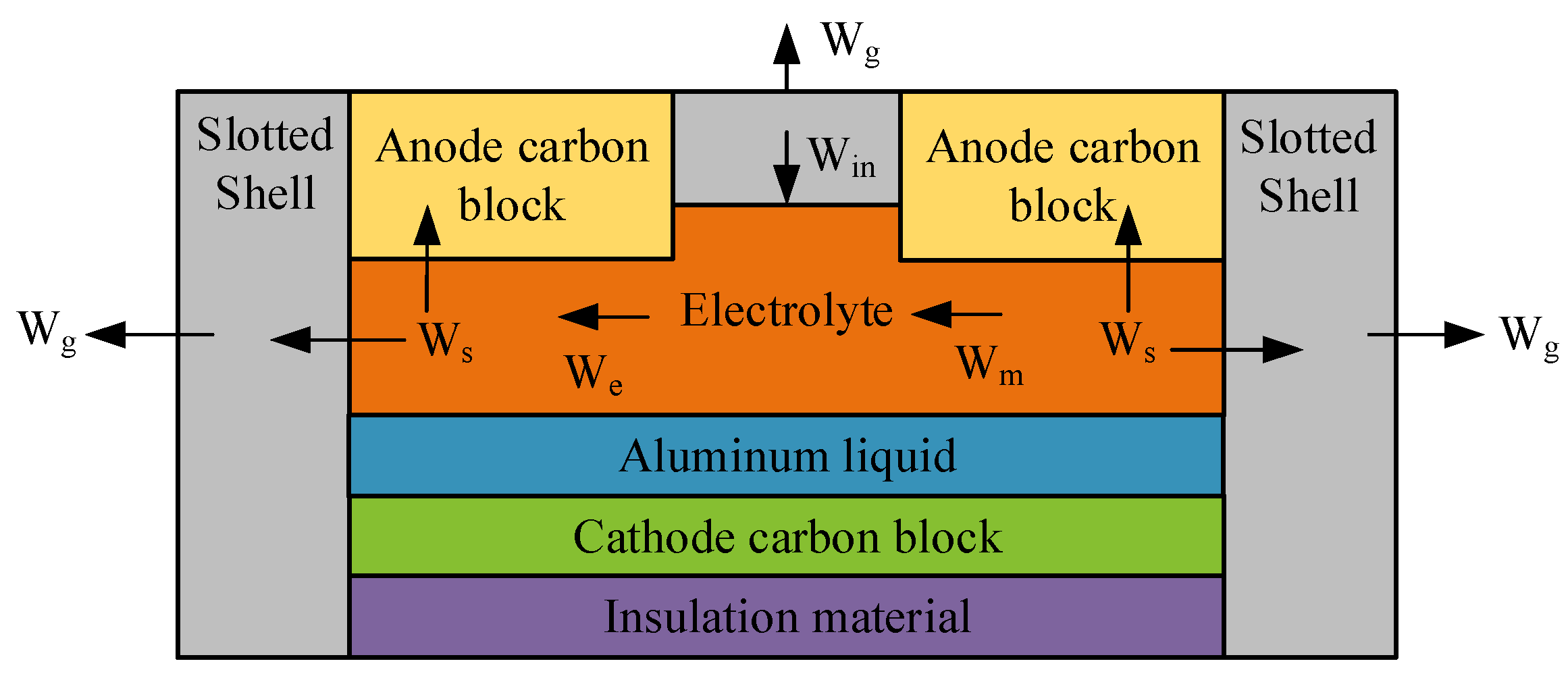
2. Electrothermal Coupling Model of Aluminum Electrolytic Cell

2.1. EA Load Regulation Characteristics

The equivalent circuit of EA is shown in Figure 1. The production of EA is usually carried out by cryolite-alumina molten salt electrolysis. Therefore, the electrolytic cell needs to maintain a certain temperature to keep the alumina in a molten state. The electrolytic tank current size is critical to the production of EA and the stability of the electrolytic cell. The current on the AC bus side is transformed and rectified and then flows into the electrolytic cell to provide energy for the electrochemical reaction of EA. The electrolytic cell is usually equivalent to a static model of a series of resistances and back electromotive force connected in series. The equivalent circuit of EA can be expressed as follows:

It can be seen from Figure 1 that the DC voltage U_D of the electrolytic cell can be expressed as follows:

$$U_D=I_{D}R+E$$

(1)

where I_D represents the DC flowing into the electrolytic cell; R is the resistance of the electrolytic cell, including ohmic resistance, bubble resistance and contact resistance; and E is the electrochemical reaction voltage drop of the electrolytic cell. The EA load power P_cell can be expressed as follows:

$$P_{\mathrm{cell}}=I_D{U}_D$$

(2)

The electrolytic cell power can be changed by adjusting the electrolytic cell current so that the EA load actively participates in the system DR. There are two ways to adjust the current: one is to adjust the on-load voltage regulating transformer, and the other is to adjust the saturated reactor, and between these, the saturated reactor has a faster adjustment speed.

In the EA islanded microgrid, the heat of the aluminum electrolytic cell mainly comes from the Joule heat generated by the current flowing through the body resistance of the electrolytic cell. The current in the electrolyzer is supplied by the CHP units and PV units. Joule heat is not only used to maintain the high temperature environment required for electrolysis, but also to compensate for the heat consumed by electrochemical reactions and heating materials. The rest is dissipated into the external environment through heat conduction and radiation. The actual heat conduction model of an aluminum electrolytic cell is complex. However, the anode/cathode carbon blocks, the cell shell, the electrolyte, and the aluminum liquid are the main energy-consuming and heat-dissipating modules in the aluminum electrolytic cell, accounting for approximately 90% of the total energy consumption. Among them, the electrolyte and the aluminum liquid have liquid properties. Moreover, the thermal conductivity coefficients of the electrolyte and the aluminum liquid are similar, and they are in contact with each other. Therefore, the temperature distributions of the two are similar. The anode carbon blocks and the cell shell, on the other hand, have solid properties. They are both in contact with the high-temperature electrolyte or aluminum liquid, and the temperature gradually decreases from the inside to the outside while dissipating heat to the external environment. Therefore, in order to better analyze the electro-thermal coupling relationship of the electrolyzer, it is simplified to divide the electrolyzer into a liquid system and a solid system [21]. The liquid system includes the electrolyte and the aluminum liquid, and the solid system includes the tank shell, anode carbon block, cathode carbon block and thermal insulation material. Since there is insulation material at the bottom of the aluminum electrolytic cell, the heat dissipation is relatively small [22,23]. Therefore, this paper ignores the heat dissipation of the bottom cathode carbon block and insulation material. A schematic diagram of heat transfer between the internal modules and between the interior and exterior of the electrolyzer is shown in Figure 2.

2.2. Liquid System

Taking the liquid as the object of study, this paper assumes that the temperature change of the molten aluminum is equal to that of the electrolyte. The heat calculation formula is as follows:

$$W_{in}-W_{out}=\left(c_e{m}_e\right)\Delta T_e$$

(3)

$$W_{in}=I_l(U_{cell}-E)\Delta t$$

(4)

$$W_{out}=W_e+W_m+W_s$$

(5)

where W_in is the Joule heating resulting from the thermal effect of the input current; W_out is the heat dissipated inside the aluminum electrolytic cell; W_e is the heat absorbed by the electrochemical reaction; W_m is the heat consumed by the heating material; W_s is the heat transfer from the liquid system to the solid system. c_e is the specific heat capacity of the liquid system; m_e is the quality of the liquid system; ΔT_e is the temperature change of the liquid system; I_l is the current of the electrolyzer; l is the electrolytic cell index; U_cell is the voltage of the electrolyzer; E is the back electromotive force of the electrolyzer; and Δt is the unit time.

The total reaction equation for EA is:

$${2\mathrm{Al}}_2{\mathrm{O}}_3{+3\mathrm{C}=4\mathrm{Al}+3\mathrm{CO}}_2$$

(6)

The aluminum output per electrolyzer per unit of time can be expressed as follows:

$$M=Q{I}_l\eta \Delta t$$

(7)

where η is the effective rate of the electrolyzer current. The liquid aluminum will participate in the secondary reaction and be consumed, resulting in an effective rate less than 1. Q is the faraday equivalent of electrolytic aluminum and it is about 0.0000935 g/C.

Considering the secondary reaction of EA, the heat consumed by the electrochemical reaction of EA can be expressed as follows:

$$W_e=\left(\Delta P_l^{reac}-\Delta {P_l^{reac}}^{\prime }\left(1-\eta \right)\right)M\Delta t$$

(8)

where $\Delta P_l^{reac}$ is the power consumption of the chemical reaction for producing one ton of aluminum, which is about 5.63 kWh/kg (Al), and $\Delta {P_l^{reac}}^{\prime }$ is the power consumption of the secondary chemical reaction for producing one ton of aluminum. The secondary reaction of liquid aluminum is an exothermic reaction, and the heat release is converted into electrical energy of about 4.32 kWh/kg (Al).

The amount of heat consumed by heating the material can be expressed as follows:

$$W_m=\Delta P_l^{heat}M\Delta t$$

(9)

where Δ$P_l^{heat}$ is the power required to produce one ton of aluminum heating material, which is about 0.7 kWh/kg (Al).

The heat between the liquid and solid systems is transferred in a convective manner, which is calculated by the convective heat transfer formula:

$$W_s=\left(l_a{S}_a+l_b{S}_b+l_c{S}_c\right)\left(T_e-T_s\right)\Delta t$$

(10)

where T_e and T_s are the average temperature of the liquid system and the solid system, respectively; l_a, l_b, and l_c are the convective heat transfer coefficients between the electrolyte and the side tank shell, between the aluminum liquid and the side tank shell, and between the electrolyte and the top anode carbon block, respectively; S_a, S_b, and S_c are the heat exchange areas between the electrolyte and the side tank shell, between the aluminum liquid and the side tank shell, and between the electrolyte and the top anode carbon block, respectively.

The analytical formula for the dynamic change of temperature of the liquid system can be obtained by sorting out the above formula (Δt is taken as 1 h here):

$$\begin{array}{l}{T}_{e,t+1}-T_{e,t}={\displaystyle \frac{\left(U_{cell}-E\right)I_{l,t}-Q\eta \left(\Delta P_l^{reac}+\Delta P_l^{heat}-\Delta {P_l^{reac}}^{\prime }\left(1-\eta \right)\right)I_{l,t}}{c_e{m}_e}}\\ -{\displaystyle \frac{\left(l_a{S}_a+l_b{S}_b+l_c{S}_c\right)\left(T_{e,t}-T_{s,t}\right)}{c_e{m}_e}}\end{array}$$

(11)

2.3. Solid System

Taking the solid system as the research object, the heat calculation formula is as follows:

$$W_s-W_g=c_s{m}_s\Delta T_s$$

(12)

$$W_g=l_s\left(T_s-T_0\right)S_s\Delta t$$

(13)

where W_g is the heat transferred by the solid system to the external environment; c_s is the specific heat capacity of the solid system; m_s is the mass of the solid system; ΔT_s is the change in the average temperature of the solid system; l_s is the convective heat transfer coefficient between the solid system and the external environment; S_s is the heat transfer area between the solid system and the external environment; and T₀ is the average temperature of the external environment.

The analytical formula for the dynamic change of temperature of the solid system can be obtained as follows:

$$T_{s,t+1}-T_{s,t}={\displaystyle \frac{\left(l_a{S}_a+l_b{S}_b+l_c{S}_c\right)\left(T_{e,t}-T_{s,t}\right)}{c_s{m}_s}}-{\displaystyle \frac{l_s{S}_s\left(T_{s,t}-T_0\right)}{c_s{m}_s}}$$

(14)

From Equations (11) and (14), we get the following:

$$T_{e,t+2}=a{T}_{e,t+1}-b{T}_{e,t}+c{I}_{l,t+1}-d{I}_{l,t}+K$$

(15)

$$\left\{\begin{array}{l}a=2-{\displaystyle \frac{l_a{S}_a+l_b{S}_b+l_c{S}_c}{c_e{m}_e}}-{\displaystyle \frac{l_a{S}_a+l_b{S}_b+l_c{S}_c+l_s{S}_s}{c_s{m}_s}}\\ b=1-{\displaystyle \frac{l_a{S}_a+l_b{S}_b+l_c{S}_c}{c_e{m}_e}}-{\displaystyle \frac{l_a{S}_a+l_b{S}_b+l_c{S}_c+l_s{S}_s}{c_s{m}_s}}+{\displaystyle \frac{\left(l_a{S}_a+l_b{S}_b+l_c{S}_c\right)l_s{S}_s}{c_e{m}_e{c}_s{m}_s}}\\ c={\displaystyle \frac{U_{cell}-E-Q\eta \left(\Delta P_l^{reac}+\Delta P_l^{heat}-\Delta {P_l^{reac}}^{\prime }\left(1-\eta \right)\right)}{c_e{m}_e}}\\ \begin{array}{l}d={\displaystyle \frac{U_{cell}-E-Q\eta \left(\Delta P_l^{reac}+\Delta P_l^{heat}-\Delta {P_l^{reac}}^{\prime }\left(1-\eta \right)\right)}{c_e{m}_e}}\left(1-{\displaystyle \frac{l_a{S}_a+l_b{S}_b+l_c{S}_c+l_s{S}_s}{c_s{m}_s}}\right)\\ K={\displaystyle \frac{\left(l_a{S}_a+l_b{S}_b+l_c{S}_c\right)l_s{S}_s{T}_0}{c_e{m}_e{c}_s{m}_s}}\end{array}\end{array}\right.$$

(16)

where a, b, c, d, e, f, and K are constants.

As can be seen from the above equation, the electrolyte temperature at t + 2 is not only related to the electrolyte temperature and the intensity of the incoming current at t + 1, but also to the electrolyzer state at t. And the electrolyte temperature is related to multiple state variables (e.g., T_e,t, T_e,t+1, I_t and I_t+1). Equation (15) is a linear equality, and there is no need for convex relaxation or linearization treatment.

3. CHP Units and EA Load Dispatch Model

3.1. Industrial Microgrid System Structure

This paper takes an industrial island microgrid as the research object, which includes CHP units and PV units, of which the PV installed capacity accounts for a high proportion. The load includes the EA load, interruptible load and other loads, among which the EA load accounts for more than 80% of the total system load. It is the main DR resource of this paper. The thermal power of the CHP unit is mainly used to produce alumina, so the thermal power regulation part of the CHP unit is not considered in this paper. The specific industrial microgrid network structure is shown in Figure 3.

3.2. CHP Units Model

CHP units are usually divided into two types: back-pressure CHP units and pumped-condensing CHP units, and pumped-condensing CHP units can simultaneously satisfy the electric load and heat load demand. Due to the existence of a certain coupling relationship between its electric power output and heat output, it makes the unit’s electric power regulation ability limited. In order to realize the thermal and electric decoupling of CHP units, CHP units are usually operated in conjunction with other types of units or equipment.

The total output power of the CHP unit i can be expressed as follows:

$$P_{i,t}=P_{i,t}^e+c_{v,i}{P}_{i,t}^h$$

(17)

where P_i,t is the total power output of the CHP unit in time period t; $P_{i,t}^e$ is the electric power output of the CHP unit in time period t; $P_{i,t}^h$ is the thermal power output of the CHP unit in time period t; and c_v,i is the coefficient of the electrical and thermal characteristics of the CHP unit.

The CHP unit coal cost C_chp,rm can be expressed as follows:

$$C_{chp,rm}={\gamma }^{fule}{\displaystyle \sum _{t=1}^T{\displaystyle \sum _{i=1}^N[A_i+B_i{\mathrm{P}}_{i,t}^e+C_i{P}_{i,t}^h+D_i{({\mathrm{P}}_{i,t}^e)}^2+E_i{\mathrm{P}}_{i,t}^e{P}_{i,t}^h+F_i{(P_{i,t}^h)}^2]}}$$

(18)

where γ^fule is the coal price and A_i, B_i, C_i, D_i, E_i, and F_i are the coal consumption coefficients of the CHP unit i.

The carbon emission E_chp of CHP units can be calculated by the following formula:

$$E_{chp}={\displaystyle \sum _{t=1}^T{\displaystyle \sum _{i=1}^N\left[a_i+b_i{P}_{i,t}^e+c_i{(P_{i,t}^e)}^2+d_i{P}_{i,t}^h+f_i{(P_{i,t}^h)}^2\right]}}$$

(19)

where a_i, b_i, c_i, d_i, e_i, and f_i are the carbon emission coefficients for CHP unit i.

3.3. EA Load Model

Normally, the power of the EA load is worked at the maximum value to ensure the highest aluminum production. However, the EA load belongs to the flexible load, which has the advantages of fast regulation speed and large regulation capacity. The general regulation range can reach ±20%. Therefore, the EA load is considered to participate in the DR of the system and smooth out fluctuations in renewable energy output.

(1) The EA plant’s revenue comes mainly from aluminum products. It earns profit B_ea, which can be expressed as follows:

$$B_{ea}={\gamma }^{sale}{\displaystyle \sum _{l=1}^L{\displaystyle \sum _{t=1}^T{P}_{l,t}}/k}$$

(20)

where L is the total number of electrolytic cell series; t is the time index; T is the total dispatching time; γ^sale is the selling price per ton of EA, which is about 18,000 RBM/t; P_l,t is the electrolytic cell series l in the t time period of the electric power; and k is the coefficient of electricity consumed for each production of each ton of EA products, about 13,500 kWh/t.

(2) In the process of EA production, raw materials such as alumina and anode charcoal briquettes need to be continuously added to the electrolytic cell, and the raw materials’ cost C_ea,rm can be expressed as follows:

$$C_{ea,rm}={\gamma }^m{\displaystyle \sum _{l=1}^L{\displaystyle \sum _{t=1}^T{P}_{l,t}}/k}$$

(21)

where γ^m is the raw material cost coefficient of producing a ton of EA.

(3) The switching equipment adjustment cost can be expressed in terms of the number of EA load ramps:

$$C_{ea,eq}={\gamma }^{eq}{\displaystyle \sum _{l=1}^L{\displaystyle \sum _{t=1}^T\left({\alpha }_{l,t}+{\beta }_{l,t}\right)}}$$

(22)

where γ^eq is the switching equipment adjustment cost coefficient. α_l,t and β_l,t are the EA load up-climbing and down-climbing state, respectively, and they are binary variables, where 1 indicates the EA load in the up-climbing or down-climbing state and 0 indicates the EA load in the smooth state.

(4) The electrolytic cell is an important production equipment for EA. The production process of EA will inevitably cause a certain life loss of the electrolytic cell. Therefore, the electrolytic cell needs to be maintained regularly. The required unit power operation and maintenance cost C_ea,om can be expressed as follows:

$$C_{ea,om}={\gamma }^{op}{\displaystyle \sum _{l=1}^L{\displaystyle \sum _{t=1}^T{P}_{l,t}}}$$

(23)

where γ^op is the operation and maintenance cost coefficient.

(5) In the aluminum industry, alumina and EA are the main carbon emission links. This paper only considers the carbon emission cost of EA. The sources of carbon emissions from EA mainly include carbon anode consumption, the anode effect generated during the production of EA, and electricity consumption. Among them, carbon emissions due to electricity consumption are the carbon emissions generated by coal burning of CHP units, which have been described above.

The carbon emissions E_ea,c due to the consumption of carbon anodes as a raw material for EA can be expressed as follows:

$$E_{ea,c}={\displaystyle \sum _{l=1}^L{\displaystyle \sum _{t=1}^T\frac{1}{k}\times E{F}_c{P}_{l,t}\Delta t}}$$

(24)

$$E{F}_c=N{C}_c\times \left(1-S_c-A_c\right)\times {\lambda }_1$$

(25)

where EF_c is the carbon dioxide emission factor of carbon anode consumption, NC_c is the amount of anode carbon in the electrolyzer consumed in the production of each ton of aluminum, S_c is the average sulfur content of the carbon anode, A_c is the average ash content of the carbon anode, and λ₁ is a constant coefficient. According to the recommended value of the China Nonferrous Metals Industry Association, NC_c can be taken as 0.42 t(C)/t(Al), S_c can be taken as 2%, and A_c can be taken as 0.4%.

The carbon emissions of the anodic effect that occurs during the production of EA can be expressed as:

$$E_{ea,cf}=\left({\lambda }_2\times E{F}_{C{F}_4}+{\lambda }_3\times E{F}_{C_2{F}_6}\right)\times {\displaystyle \sum _{l=1}^L{\displaystyle \sum _{t=1}^T{P}_{l,t}}}\times {\displaystyle \frac{1}{k}}$$

(26)

where λ₂ and λ₃ are the greenhouse effect conversion indices of CF₄ and C₂F₆, respectively; EF_CF4 is the CF₄ emission factor; and EF_C2F6 is the C₂F₆ emission factor. According to the recommended value of the China Nonferrous Metals Industry Association, EF_CF4 can be taken as 0.034 kg (CF₄)/t(Al) and EF_C2F6 can be taken as 0.0034 kg(C₂F₆)/t(Al).

4. Multi-Timescale Optimal Dispatch Model for Industrial Islanded Microgrids

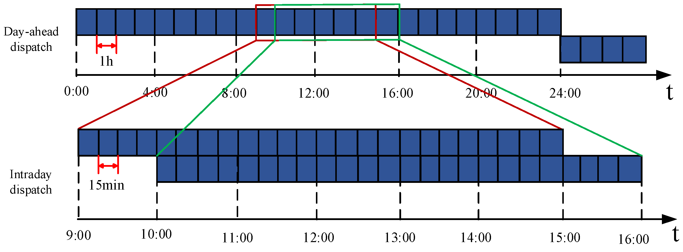
4.1. Multi-Timescale Rolling Dispatch Strategy

In order to reduce the impact of PV forecasting errors on the system, this paper adopted a day-ahead and intraday multi-timescale dispatching method, taking advantage of the rapid regulation capability of EA loads to respond in real time to the changes in PV power in the system, so as to improve the utilization rate of PV in isolated power grids.

Day-ahead dispatching plan: Dispatching optimization is carried out based on the day-ahead forecast data of PV and loads. It is executed once a day with a time resolution of 1 h. The main tasks of day-ahead dispatching are to determine the start and stop plan of the CHP units and the dispatching plan of interruptible loads.

Intraday dispatching plan: Based on the results of day-ahead dispatching and the latest forecast data of PV and loads, intraday dispatching reruns multiple rolling dispatching within a short period of time before the system executes the plan, so as to correct the day-ahead dispatching plan. In this paper, the intraday dispatching cycle is set to 6 h, with a time resolution of 15 min, and it is updated every 1 h. For example, the first rolling dispatching period is from the 1st h to the 6th h, the second rolling dispatching period is from the 2nd h to the 7th h, and so on. A total of 19 dispatching operations need to be completed, and only one dispatching is carried out for the last 6 h. However, except for the last dispatching, the system only executes the dispatching scheme for the first hour each time, promptly correcting the output of the CHP units and the regulating power of the EA loads.

The day-ahead and intraday dispatching strategies are shown in Figure 4 and Figure 5.

4.2. Day-Ahead Dispatch Model

(1)

Objective function

In this paper, the optimization goal of day-ahead scheduling is to maximize the operating profit of the island microgrid system, and its objective function is as follows:

$$\max F_1=B_{ea}-\left(\begin{array}{l}{C}_{chp,rm}+C_{ea,rm}+C^{pw}{\displaystyle \sum _{t=1}^T{\displaystyle \sum _{i=1}^N{P}_{i,t}}}+C^{sw}{\displaystyle \sum _{t=1}^T{P}_t^{sv}}+C_{ea,eq}+C_{ea,om}\\ +C^{scut}{\displaystyle \sum _{t=1}^T{P}_t^{svd}}+{\gamma }^c\left(E_{ea,c}+E_{ea,cf}+E_{chp}\right)\end{array}\right)$$

(27)

where F₁ is the day-ahead dispatching objective function, C^pw is the coefficient of maintenance cost per unit of power for CHP units, C^sw is the coefficient of maintenance cost per unit of power for PV units, $P_t^{sv}$ is the PV power forecast, C^scut is the penalty price for curtailing PV power, $P_t^{svd}$ is the PV power curtailment, and γ^c is the carbon emission price coefficient.

(2)

Constraints

(1) The power balance constraints are as follows:

$${\displaystyle \sum _{i=1}^N{P}_{i,t}^e}+P_t^{sv}={\displaystyle \sum _{l=1}^L{P}_{l,t}}+L_t^{in}+L_t^{oth}$$

(28)

where $L_t^{in}$ is an islanded microgrid interruptible load and $L_t^{oth}$ is other loads on the islanded microgrid, which are considered to remain unchanged.

(2) CHP units power constraints

The regulation range of the electrical output of the condensing CHP units will be constrained by the thermal output. Therefore, the operating range of the CHP units is a quadrilateral, and in order to ensure that the CHP units do not go beyond their operating range, it is necessary to constrain their electrical and thermal power.

$$\max (U_{i,t}{P}_{i\min }^e-c_2{P}_{i,t}^h,c_3(P_{i,t}^h-U_{i,t}{P}_{i0}^h))\le P_{i,t}^e\le U_{i,t}{P}_{i\max }^e-c_1{P}_{i,t}^h$$

(29)

$$0\le P_{i,t}^h\le U_{i,t}{P}_{i\max }^h$$

(30)

where c₁, c₂ and c₃ are the slopes of the three curves in the operating interval of the CHP unit, which characterize the coupling relationship between the electric power and the thermal power; $P_{imax}^e$ and $P_{imin}^e$ are the maximum and minimum electric power when the thermal output of the CHP unit i is zero; $P_{imax}^h$ is the maximum value of the thermal output of the CHP unit i; $P_{i0}^h$ is a constant value, which is determined by the characteristics of the unit; U_i,t is the start/stop status of the CHP units and is a binary variable, with 1 indicating on and 0 indicating off.

(3) The CHP units power ramping constraints are as follows:

$$-P_i^{edw}\le P_{i,(t+1)}^e-P_{i,t}^e\le P_i^{eup}$$

(31)

where $P_i^{eup}$ and$P_{edw}$ I, respectively, represent the maximum upward and downward power ramp rates of CHP units i.

(4) The CHP unit start/stop time constraints are as follows:

$$\left\{\begin{array}{c}{\displaystyle \sum _{k=t}^{t+T_{i,on}-1}{U}_{i,k}}\ge T_{i,on}\left(U_{i,t}-U_{i,t-1}\right)\\ {\displaystyle \sum _{k=t}^{t+T_{i,off}-1}(1-U_{i,k})}\ge T_{i,off}\left(U_{i,t-1}-U_{i,t}\right)\end{array}\right.$$

(32)

where T_m,on and T_m,off are the minimum start and stop times of the CHP units, respectively.

(5) PV constraints

The actual output of PV power during each time period cannot exceed the maximum value of PV output power during that time period.

$$0\le P_t^{sv}\le P_{t,\max }^{sv}$$

(33)

where $P_{t,max}^{sv}$ is the maximum power output.

(6) EA load constraints

The EA load regulation range is limited. If the EA load power is too low or too high, this will affect the safe operation of the electrolyzer. Therefore, it needs to limit the EA load power within a certain range:

$$\left\{\begin{array}{l}{P}_{l\mathit{min}}\le P_{l,t}\le P_{l\mathit{max}}\\ P_{l,t}=U_l{I}_{l,t}\end{array}\right.$$

(34)

where P_lmax is the maximum power of the EA load, P_lmin is the minimum power of the EA load, I_l,t is the current intensity of the electrolyzer series l passed in time period t, and U_l is the electrolyzer voltage and is regarded as a constant here.

(7) Power ramping and number of adjustments of EA load constraints

For the sake of production stability, the EA load should not be adjusted frequently, and it should be controlled not to exceed the maximum number of adjustments in one dispatching cycle.

$$-{\alpha }_{l,t}{P}_l^{dw}\le P_{l,t}-P_{l,t-1}\le {\beta }_{l,t}\Delta P_l^{up}$$

(35)

$$\left\{\begin{array}{c}{\alpha }_{l,t}+{\beta }_{l,t}\le 1\\ {\displaystyle \sum _{t=2}^T\left({\alpha }_{l,t}+{\beta }_{l,t}\right)\le m_l}\end{array},\mathrm{t}=2,3,\cdots \mathrm{T}\right.$$

(36)

where $P_l^{up}$ and $P_l^{dw}$ are the upward and downward ramp rate limiting values of the EA load power, respectively, and m_l is the maximum number of adjustments of the EA load in a scheduling cycle.

(8) Temperature constraint

In order to ensure the safe operation of EA production, we constructed an electrolyte temperature constraint and incorporated it into the optimized scheduling model. The initial and boundary conditions for the electrolyte temperature are set as follows:

$$\left\{\begin{array}{l}{I}_{l,init}=I_{\mathit{max}}\\ T_{e,\mathrm{init}}=T_{e,1}=940\\ T_{e,2}=a{T}_{e,1}-b{T}_{e,\mathrm{init}}+c{I}_{l,1}-d{I}_{l,init}+K\\ \begin{array}{l}{T}_{e,t+2}=a{T}_{e,t+1}-b{T}_{e,t}+c{I}_{l,t+1}-d{I}_{l,t}+K,t\in [1,\mathrm{T}-2]\\ T_{e,\mathit{min}}\le T_{e,t}\le T_{e,\mathit{max}}\end{array}\end{array}\right.$$

(37)

where T_e,min and T_e,max are the minimum and maximum allowable values of the electrolyte temperature, respectively, and T_e,min and T_e,max are 910 °C and 960 °C, respectively.

(9) Thermal balance constraints

In the EA load dispatch model, a heat balance constraint is used to ensure the safe production of aluminum electrolysis. A minimum energy supply to the electrolyzer is guaranteed for a certain period of time [11].

$${\eta }^{eh}{\displaystyle \sum _{l=1}^L{\displaystyle \sum _{t_1=t-\tau +1}^t{P}_{l,t_1}}}>=E_{\tau \min },\mathrm{t}\ge \tau$$

(38)

where η^eh is the efficiency of electro-thermal conversion; τ is the time for the electrolyzer to maintain thermal balance, and it is taken as 4 h here; and E_τmin is the minimum energy input required by the electrolyzer to maintain the thermal balance during the consecutive τ time periods.

(10) Aluminum production constraints

The participation of EA in DR will affect the production of aluminum products. To ensure that EA participates in the system’s DR without affecting the production plan, it is necessary to impose certain constraints on the daily production of aluminum products. Due to the direct relationship between energy consumption and the production of EA, the constraints can be expressed as follows:

$$\mu {\displaystyle \sum _{t=1}^T{P}_{l\max ,t}}\le {\displaystyle \sum _{t=1}^T{P}_{l,t}}\le {\displaystyle \sum _{t=1}^T{P}_{l\max ,t}}$$

(39)

where μ is a proportionality coefficient.

(11) The branch current constraint is as follows:

$$\left|S·P_{CHP}+S·{\mathrm{P}}_{PV}-S·{\mathrm{P}}_{EA}-S·P_L\right|\le L_{\max }$$

(40)

where S is the sensitivity matrix, P_CHP is the thermal unit power matrix, P_PV is the wind farm power matrix, P_EA is the aluminum electrolytic cell power matrix, P_L is the load power matrix, and L_max is the maximum branch current matrix.

(12) The interruptible load constraint is as follows:

$$0\le L_t^{in}\le L_{t,\max }^{in}$$

(41)

where $L_{t,max}^{in}$ is the maximum interruptible load power.

(3)

Model solution

The decision variables of the day-ahead optimal dispatching model include the start–stop states of combined CHP units, the output power of CHP units, the regulation power of EA loads, and the regulation power of interruptible loads. Since this model is a mixed-integer linear model, the CPLEX solver can be used for solving. As a result, the start–stop states of CHP units, the output power plan of CHP units, the regulation power of EA loads, and the regulation power of interruptible loads can be obtained. Among them, the start–stop states of CHP units and the regulation power of interruptible loads are input as known quantities into the intraday optimal dispatching model, and other decision variables are continuously solved in the intraday optimal dispatching model.

4.3. Intraday Dispatching Model

(1)

Objective function

The intraday dispatch also takes maximizing the operating profit of the industrial microgrid system as the optimization objective.

$$\max F_2=B_{ea}-\left(\begin{array}{l}{C}_{chp,rm}+C_{ea,rm}+C^{pw}{\displaystyle \sum _{t=1}^T{\displaystyle \sum _{i=1}^N{P}_{i,t}}}+C^{sw}{\displaystyle \sum _{t=1}^T{P}_t^{sv}}+C_{ea,eq}+C_{ea,om}\\ +C^{scut}{\displaystyle \sum _{t=1}^T{P}_t^{svd}}+{\gamma }^c\left(E_{ea,c}+E_{ea,cf}+E_{chp}\right)\end{array}\right)$$

(42)

where F₂ is the intraday dispatching objective function.

(2)

Constraints

(1) The real-time power balancing constraint is as follows:

$${\displaystyle \sum _{i=1}^N{P}_{i,t}^e}+{\displaystyle \sum _{i=1}^N\Delta P_{i,t}^e}+{P_t^{sv}}^{\prime }={\displaystyle \sum _{l=1}^L{P}_{l,t}}+{\displaystyle \sum _{l=1}^L\Delta P_{l,t}}+L_t^{in}+L_t^{oth}$$

(43)

where $\Delta P_{i,t}^e$ is the CHP unit power regulation, ΔP_l,t is the EA load power regulation, and ${P_t^{sv}}^{\prime }$ is PV forecast power for the current dispatch period.

(2) Other constraints

Different from the day-ahead optimal dispatching model, the constraint conditions do not include the start–stop time constraints of CHP units and the interruptible load constraints. Other constraint conditions are the same as those in the day-ahead optimal dispatching model.

(3)

Model solution

Different from the day-ahead optimal dispatching model, the start–stop states of CHP units and the regulation power of interruptible loads in the intraday optimal dispatching model are known quantities. The CPLEX solver is also used for solving, and the correction amounts of the output power of CHP units and the regulation power of EA loads are obtained. Therefore, the intraday optimal dispatching model further adjusts the output power of CHP units and the power of EA loads on the basis of the day-ahead dispatching results to meet the system load power demand and reduce the curtailment of photovoltaic power.

5. Case Study

5.1. System Parameters

This paper takes an industrial island microgrid in a certain area of Inner Mongolia in China as a simulation case. The industrial microgrid system includes two CHP (100 MW) units and a PV power station (100 MW). Loads of the industrial microgrid system include an EA load (100 MW), interruptible load (5 MW) and other loads (18.6 MW). The parameters of the aluminum electrolytic cell temperature model can be found in Ref. [23]. Other relevant parameters are shown in

Table 1. Aluminum electrolytic cell parameters.

Parameter Name	Value	Parameter Name	Value
Number of electrolyzer series	1	Voltage of a single electrolyzer/V	4.03
Rated capacity/MW	100	Power adjustment range/%	±20
Rated current/kA	400	Climbing rate/MW/h	±20
Average voltage of a single electrolyzer/V	62	Maximum number of adjustments	12

and

Table 2. CHP unit parameters.

Unit	Maximum Electrical Power	Minimum Electrical Power	Maximum Thermal Power	Minimum Thermal Power	Climbing Rate
1	100 MW	30 MW	120 MW	40 MW	±30 MW/h
2	100 MW	30 MW	120 MW	40 MW	±30 MW/h

.

In this paper, the actual PV output data of a certain year in an Inner Mongolia region of China are used for simulation. And the typical PV output data of a certain day among them are selected as the sample of the actual PV output data for this model. It is assumed that the PV forecasting errors follow a normal distribution, and the day-ahead PV forecasting error is greater than the intraday PV forecasting error. In this paper, the day-ahead PV forecasting error is set to 10%. Then, the day-ahead PV forecasting curve is obtained by superimposing a forecasting error curve with an expected value of 0 and a standard deviation of 0.2 on the actual PV curve. The intraday PV forecasting error is set to 2%. Then, the intraday PV forecasting curve is obtained by superimposing a forecasting error curve with an expected value of 0 and a standard deviation of 0.02 on the actual PV curve. The PV output power curves are shown in Figure 6.

To facilitate the analysis, two cases are designed in the paper.

Case 1: Considering the constraints of Equation (38), the EA load participates in DR with a power adjustment range of ±20%.

Case 2: Considering the constraints of Equation (37), the EA load participates in DR with a power adjustment range of ±20%.

Case 3: Considering the constraints of Equation (37), but the EA load does not participate in the DR and remains at its rated power value.

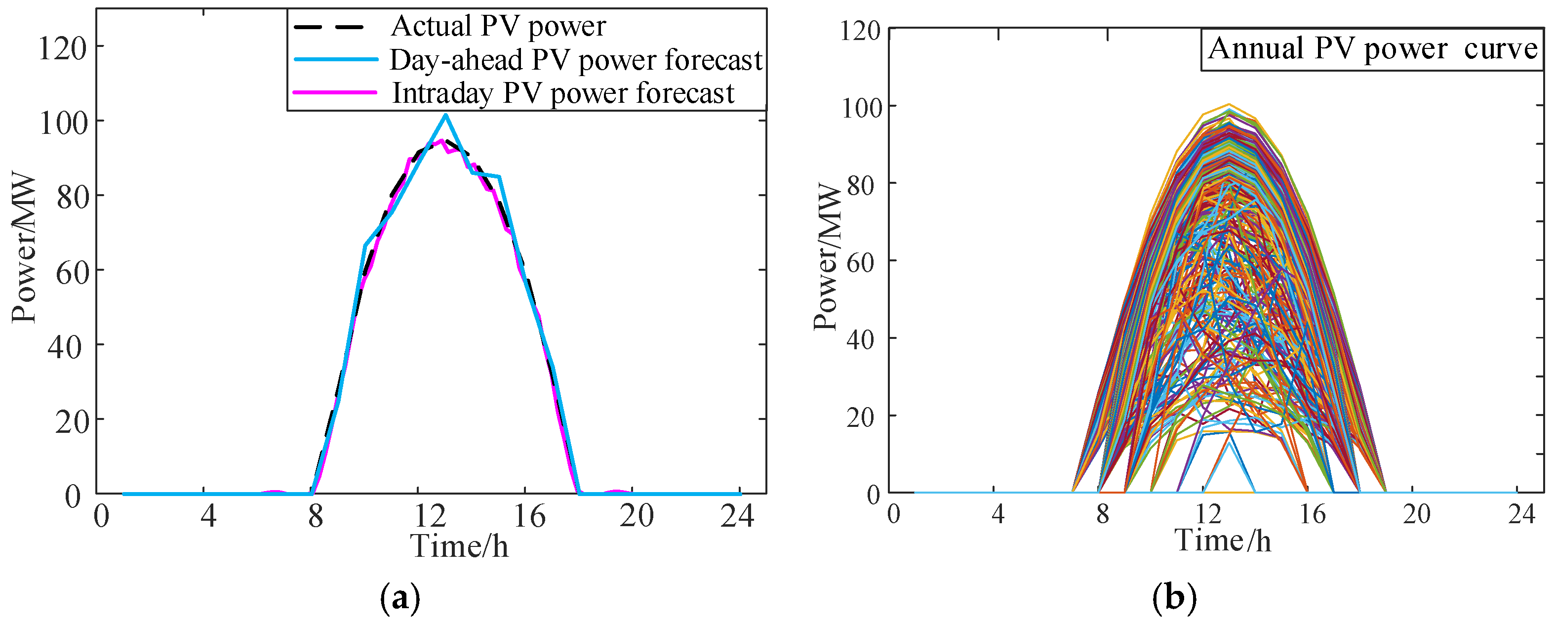
5.2. Aluminum Electrolytic Cell Temperature Model Validation

The electricity dissipation of the aluminum electrolytic cell is shown in Figure 7. It can be seen that the electric energy consumed by the electrochemical reaction is the highest. Because the temperature difference between the electrolyzer and the external environment is about 850 °C, the electric energy consumed by the transfer of the electrolyzer to the outside environment is also higher. It is necessary to consider the recovery of residual heat from the electrolyzer. The electric energy consumed by the heated material is the lowest.

The temperature dynamics along with the current change is shown in Figure 8. Under the initial value of the temperature 940 °C, when the current drops instantaneously by 20 kA and is maintained for two hours, the temperature drops by about 20 °C; when the current rises instantaneously by 20 kA and is maintained for two hours, the temperature rises by about 15 °C. When the current returns to its rated value, the temperature slowly returns to a steady state after a period of time. Therefore, the short-term and small-range changes of the electrolytic cell current have little effect on the thermal balance of the electrolyzer.

The temperature dynamics of case 1 and case 2 is shown in Figure 9. It can be seen that since case 1 takes into account the constraint of the minimum input energy of the electrolyzer, compared with case 2, the current in case 1 is significantly increased during the time periods from 3 to 5 and from 21 to 23. However, due to the lack of consideration of the temperature constraint, the temperature exceeds the lower limit during the time period from 2 to 3 and exceeds the upper limit during the time period from 16 to 17. In case 2, in order to prevent the temperature from exceeding the lower limit in the 2nd time period, the input current will be increased, and in order to prevent the temperature from exceeding the upper limit in the 16th time period, the input current will be decreased. Therefore, after case 2 takes into account the dynamic characteristics of the electrolyte temperature, in order to maintain the temperature within a reasonable range, the input current of the electrolyzer will also change correspondingly in some time periods, thus affecting the dispatching result of the EA load. But it is beneficial for improving the production safety of the electrolyzer.

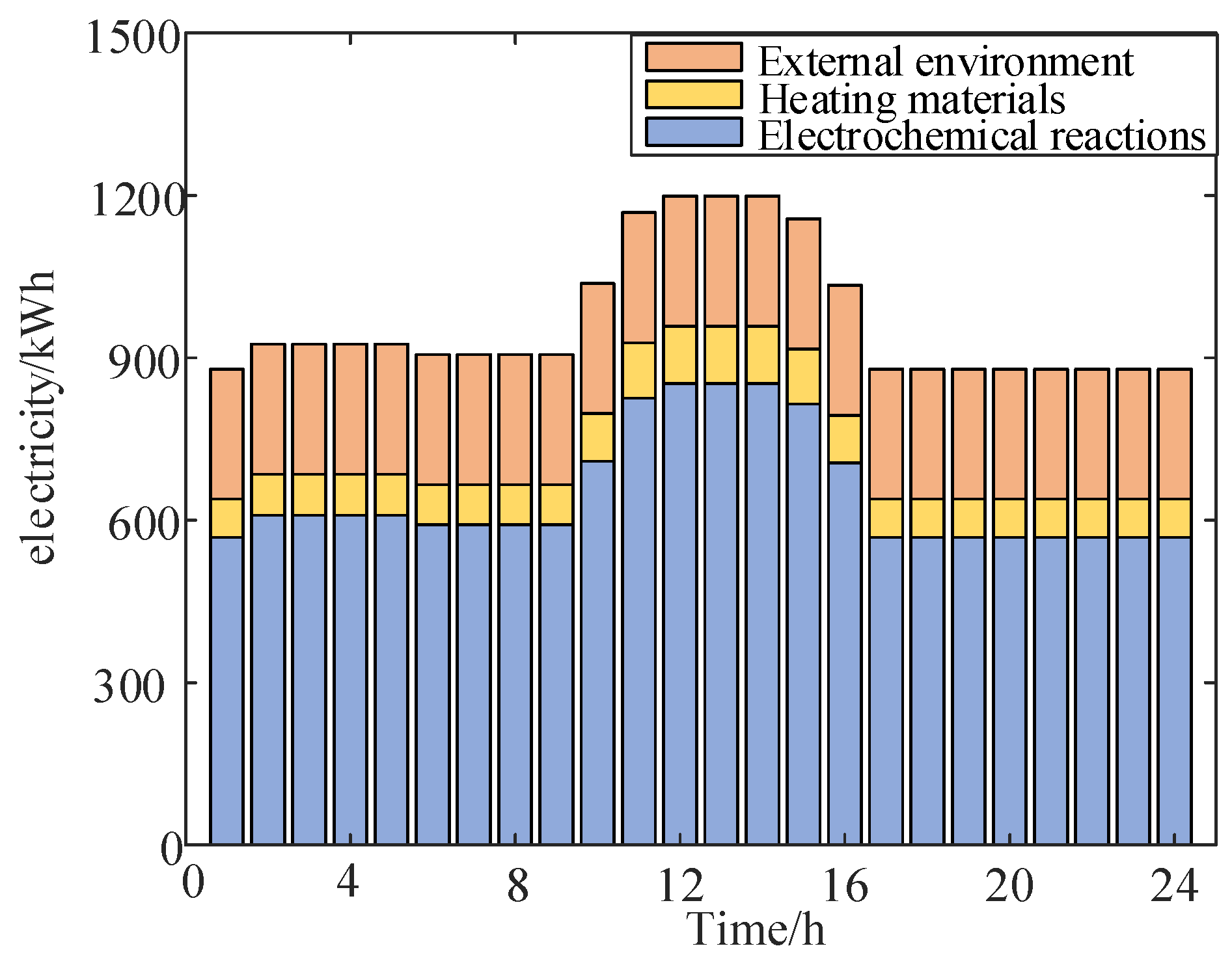
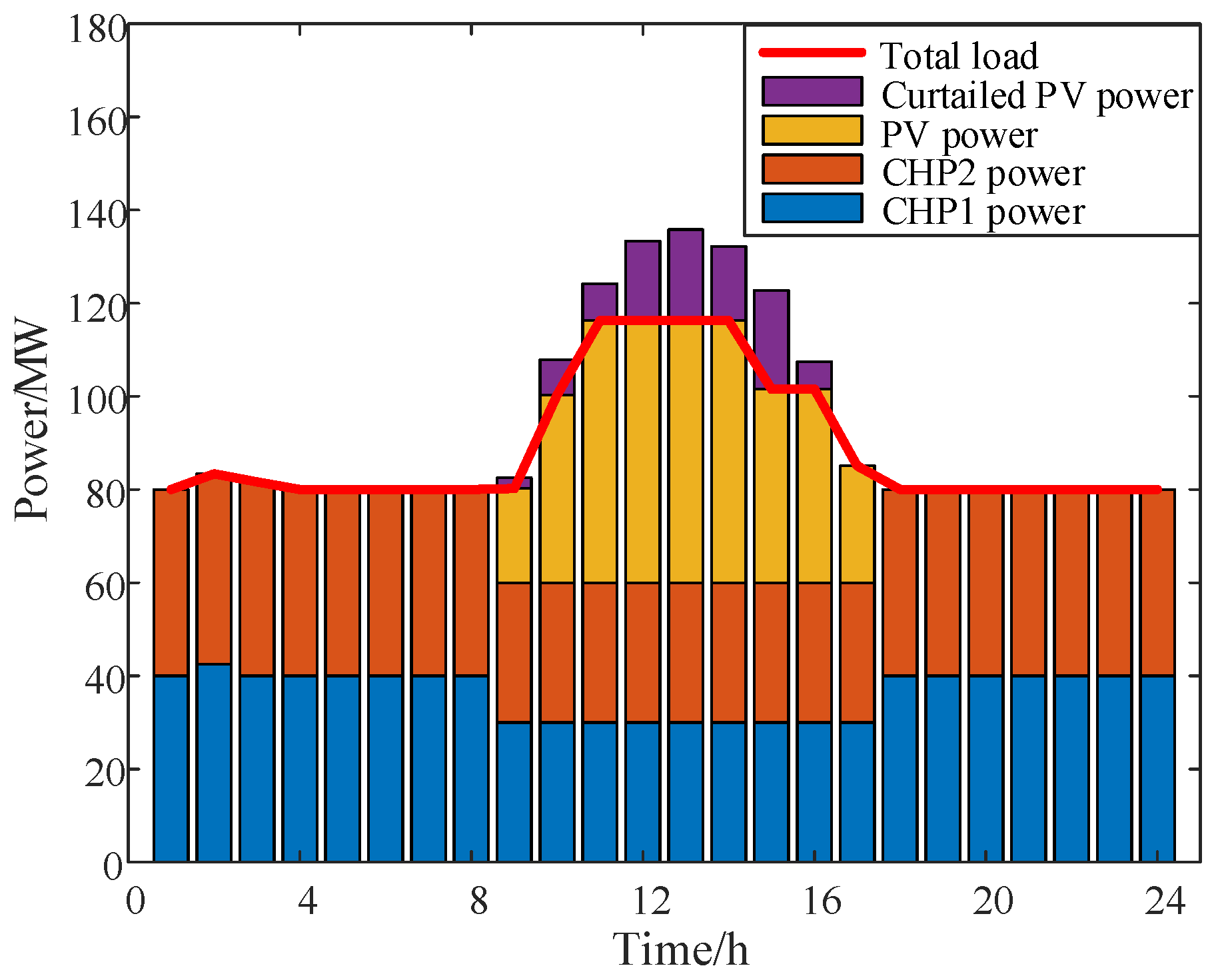
5.3. Day-Ahead Dispatch Results

The system power and load operation in two cases of the EA load, participating in DR and not participating in DR, are shown in Figure 10. It can be seen that in case 2, when the PV output is maximum, in order to fully consume the PV power, the power of the EA load will gradually increase to the maximum value, and at this time, the CHP units’ output power is the smallest. In case 3, the power of the EA load is maintained at the rated value. Due to the insufficient regulation ability of the CHP units, the system curtails the PV power seriously. Therefore, improving the flexibility of the EA load is conducive to improving the PV consumption rate.

Taking the actual PV output power data of the system in a year as an example, the islanded microgrid system day-ahead economic dispatch for one year is optimized. The optimization results for the first week of each season throughout the year are shown in Figure 11. The PV output power has great stochasticity. After the EA load participates in the DR, the EA load power tracks the fluctuation of the PV output. When the PV output increases, the EA load power is up-regulated, even running at maximum power, which is conducive to improving the system’s aluminum output. Comparatively speaking, the CHP units’ power is stable and less affected by the fluctuation of the PV output. The dispatch plan of the CHP units does not differ much every day, so the participation of the EA load in DR helps to alleviate the regulation pressure of the CHP units.

In order to further analyze the cost–benefit balance of the system, we investigated the initial investment and construction costs of the electrolytic aluminum plant, photovoltaic power station and thermal power plant. And, it was found that during the production and operation process of EA, the costs of raw materials (such as alumina and anode carbon blocks) and the cost of power consumption (such as coal consumption cost) account for about 80% of the total production and operation cost, while other costs (such as manufacturing expenses, administrative expenses, financial expenses, operating expenses, etc.) account for about 20%. Therefore, in the model of this paper, the costs of raw materials, coal consumption, operation and maintenance, curtailed photovoltaic power, and carbon emission are considered, which can be approximated as 80% of the total production and operation cost. By adding the other 20% of the total production and operation cost, the return on investment (ROI), investment payback period (IPP), and break-even point (BEP) of this project can be roughly calculated, as shown in the

Table 3. System economic analysis.

	Numeric Name	Case 2	Case 3
Investment costs/(in million RMB)	Electrolytic aluminum plant	620	620
	Thermal power plant	477	477
	Photovoltaic power station	330	330
	Total investment cost	1427	1427
Production and operation cost/(in million RMB)	Coal consumption	305.37	283.85
	Raw materials	356.76	324.44
	Curtail PV	2.04	8.09
	Carbon emissions	47.91	45.47
	Operation and maintenance	21.50	20.34
	Other	183.40	170.55
	Total cost	916.98	852.74
Revenue/(in hundred million RMB)	Total revenue	1284.33	1168.0
Economic index	Net profit/(in million RMB)	367.35	315.26
	Net profit per ton of aluminum/(in RMB)	5148.42	4858.45
	ROI/%	25.74%	22.09%
	IPP/year	<4	>4
	BEP/t(Al)	277,172.41	293,715.07

.

It can be seen that in case 2 and case 3, the carbon emission cost and raw material cost are the highest, followed by the carbon emission cost and operation and maintenance cost. Compared with case 3, case 2 takes into account the participation of the EA load in the system demand response. When the photovoltaic power output is large, the EA load will increase its power, resulting in a decrease in the curtailed photovoltaic power cost. The total production cost of case 2 is higher than that of case 3. This is because the aluminum production output in case 2 is higher than that in case 3, leading to correspondingly higher production costs. However, the production revenue obtained in case 2 is also higher. The production profit per ton of aluminum in case 2 is 5.97% higher than that in case 3. The ROI of case 2 is 25.74%, and the IPP is less than 4 years. The ROI of case 3 is 22.09%, and the IPP is more than 4 years. Therefore, the BEP of case 2 is less than that of case 3. In conclusion, after the EA load participates in the system demand response, it can increase the electrolytic aluminum production output of the system, increase the revenue, and shorten the IPP.

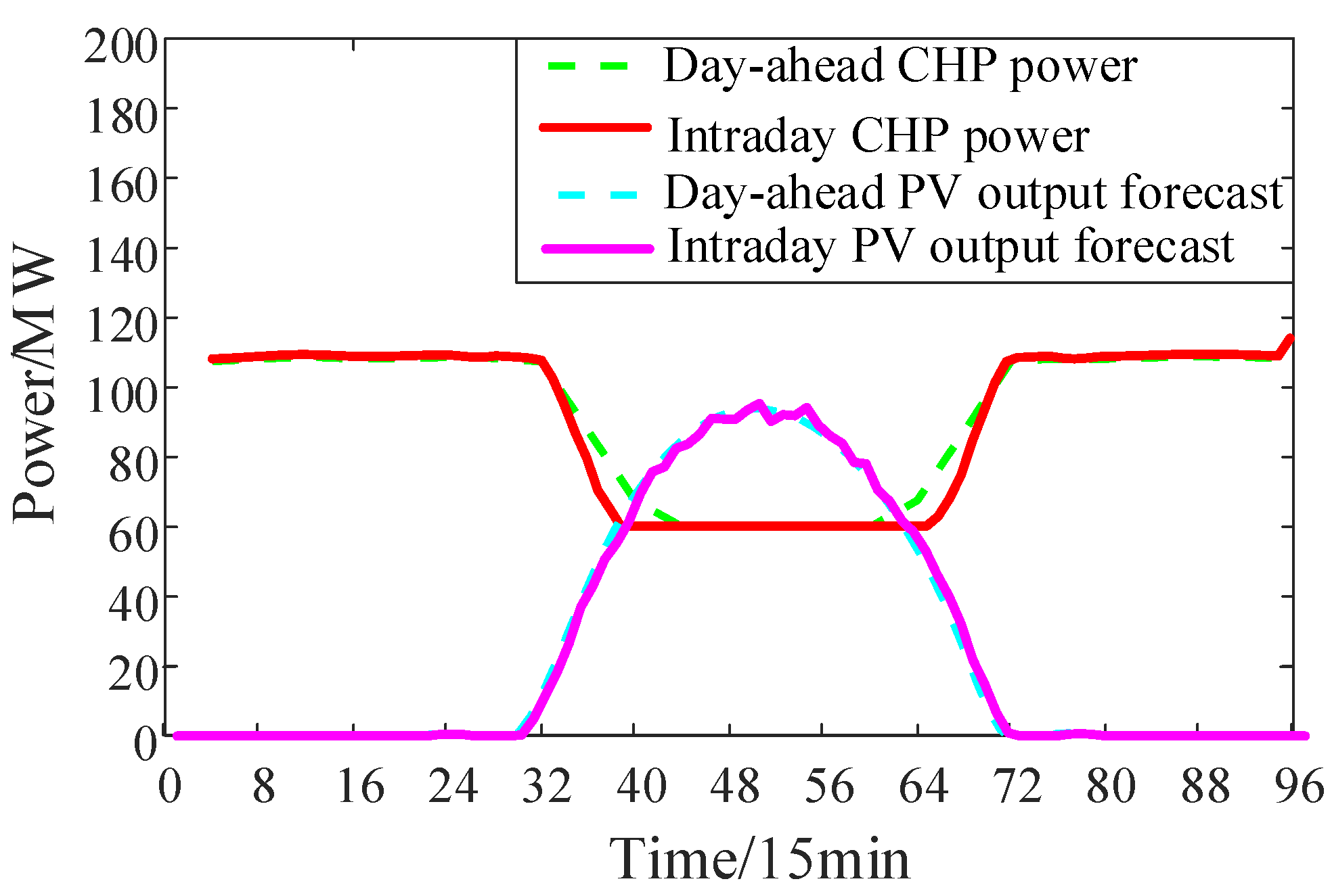
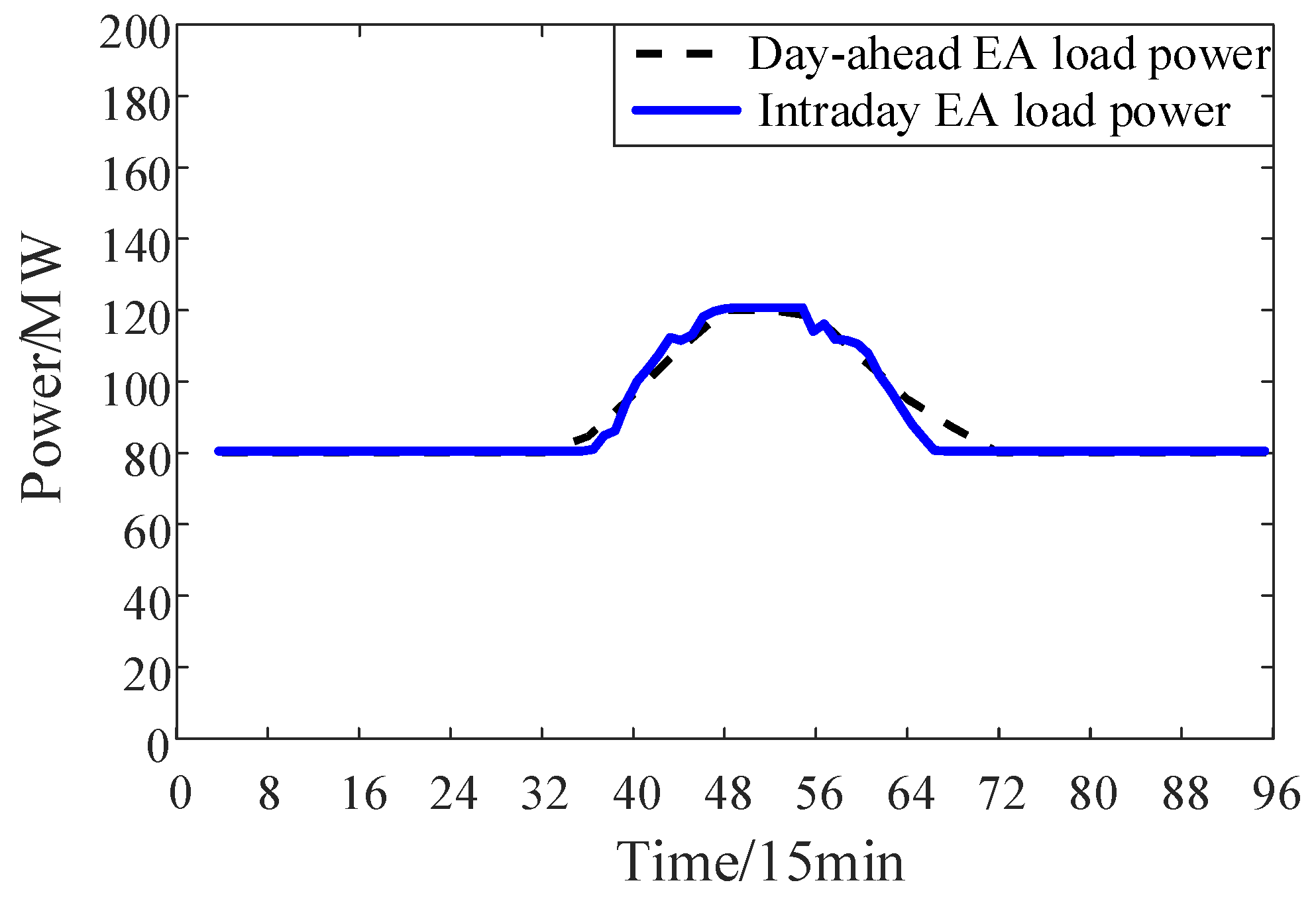
5.4. Intraday Dispatch Results

EA load regulation is fast, so the load power of the EA can respond in real time during the intraday dispatch. The day-ahead and intraday dispatch plans for CHP units and EA load in the island microgrid system is shown in Figure 12 and Figure 13. It can be seen that despite the high variability of the PV power output, the electric power output of the CHP units remains relatively stable with minimal fluctuations under both day-ahead and intraday dispatch. This is because the EA load has the ability to respond quickly, which can quickly balance the fluctuations in PV output power during intraday dispatching. It can alleviate the climbing pressure of CHP units while also reducing PV curtailment. Therefore, using a multi-time scale rolling dispatching strategy, which on the basis of day-ahead dispatching, superimpose intra-day rolling dispatching, can correct the day-ahead dispatching plan according to the predicted changes in PV output power. This can gradually reduce the impact of the PV output prediction errors on system stability and improve the access capabilities of the island microgrid systems to the PV.

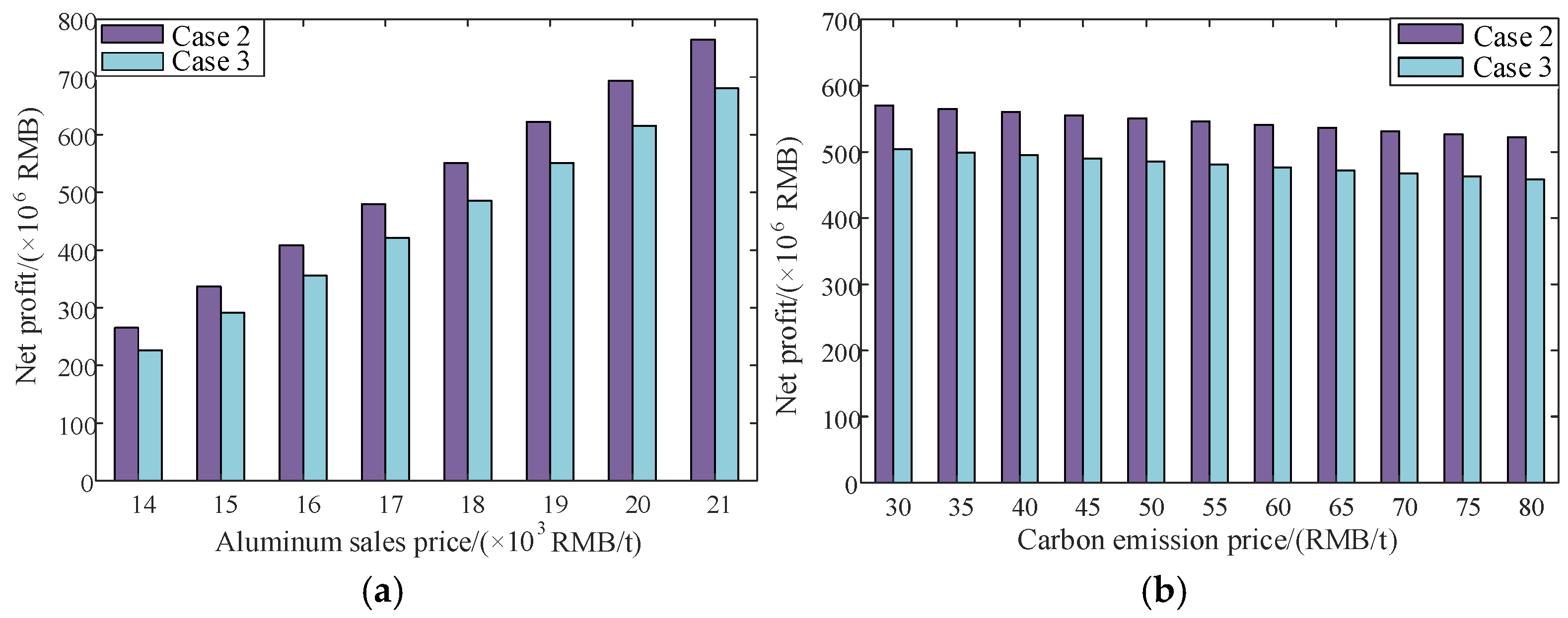
5.5. Sensitivity Analysis

We assume that due to reasons such as inspection and maintenance or operational failures, 6 sub-electrolytic cells in this aluminum electrolytic cell series need to be shut down, while the remaining 56 sub-electrolytic cells continue to operate. Using case 2’s optimization scheduling strategy, the optimization results are shown in Figure 14.

As is evident from Figure 14, after some of the electrolyzers are out of operation, the EA load power drops significantly. When the photovoltaic power generation output is high, the power of the EA load is adjusted up to the maximum value. However, there is still a substantial amount of curtailed photovoltaic power. There are mainly two reasons for this situation: Firstly, due to the constraints of the electrolyte temperature, the EA load cannot operate at the maximum power for an extended period. Secondly, influenced by the minimum power constraints of the CHP units and the minimum start/stop time constraints, the two CHP units can only operate at their minimum power levels. Therefore, when the series of electrolyzers operate under reduced load conditions, it not only increases the rate of photovoltaic power curtailment in the system but also results in a decrease in the production volume of electrolytic aluminum in the system and a reduction in profits.

Figure 15 shows the influence of different aluminum sales prices and carbon emission prices on the system’s net profit. It can be seen that as the sales price of aluminum products increases, the system’s aluminum sales revenue increases, and the net profit grows approximately linearly. This is because the production cost per ton of electrolytic aluminum remains unchanged, and the daily production output of electrolytic aluminum in the system has basically reached the upper limit. It is impossible to increase the profit by increasing the power of electrolytic aluminum production. Similarly, as the carbon emission price increases, the carbon emission cost of the system increases, leading to a decrease in the net profit. However, the decline is relatively small. Therefore, the system is more affected by the fluctuations in the sales price of electrolytic aluminum. At different aluminum prices and carbon prices, compared with case 3, the system’s net profit in case 2 is significantly higher.

6. Conclusions

In the paper, a multi-timescale optimal dispatching method considering the dynamic temperature characteristics of an aluminum electrolytic cell was proposed for an industrial isolated microgrid. The following conclusions were drawn:

• Incorporating the dynamic temperature constraints of aluminum electrolytic cells in the optimization of EA load dispatch can effectively mitigate the risk of electrolyzer temperature overruns, ensuring the safe and stable operation of the EA process.
• The participation of EA loads in system DR improves the PV consumption rate, contributing to the low-carbon and economically efficient operation of industrial islanded microgrids.
• Leveraging the high flexibility and rapid regulation capabilities of EA loads, real-time adjustments to the system’s power balance on an intraday timescale can effectively smooth out the fluctuations in PV output.

References

1. Han, J.; Yan, L.; Li, Z.; Zhang, L.; Paaso, A.; Bahramirad, S. A Multi-Timescale Two-Stage Robust Grid-Friendly Dispatch Model for Microgrid Operation. IEEE Access 2020, 8, 74267–74279. [Google Scholar] [CrossRef]
2. Zhang, J.; Tan, J.; Liu, Z.; Li, M.; Tao, Y.; Luo, T. Active Distribution Network Flexibility Evaluation Method Considering Flexibility Resource. In Proceedings of the 2022 12th International Conference on Power and Energy Systems (ICPES), Guangzhou, China, 23–25 December 2022; pp. 62–66. [Google Scholar]
3. Chen, S.; Gong, F.; Sun, T.; Yuan, J.; Yang, S.; Liu, Z. Research on the Method of Electrolytic Aluminum Load Participating in the Frequency Control of Power Grid. In Proceedings of the 2021 IEEE 2nd International Conference on Big Data, Artificial Intelligence and Internet of Things Engineering (ICBAIE), Nanchang, China, 26–28 March 2021; pp. 798–801. [Google Scholar]
4. Xu, J.; Liao, S.; Sun, Y.; Ma, X.; Gao, W.; Li, X.; Gu, J.; Dong, J.; Zhou, M. An isolated industrial power system driven by wind-coal power for aluminum productions: A case study of frequency control. In Proceedings of the 2015 IEEE Power & Energy Society General Meeting, Denver, CO, USA, 26–30 July 2015; pp. 471–483. [Google Scholar]
5. Ding, X.; Xu, J.; Sun, Y.; Liao, S.; Xia, T.; Chen, W. A Demand Side Industrial Aluminum Load Control Scheme based on Output Regulator Theory for Wind Power Smoothing. In Proceedings of the 2020 IEEE 4th Conference on Energy Internet and Energy System Integration (EI2), Wuhan, China, 30 October–1 November 2020; pp. 286–291. [Google Scholar]
6. Gong, F.; Ren, K.; Zhang, A.; Chen, S.; Feng, J.; Zhang, K.; Li, D. Review of electrolytic aluminum load participating in demand response to absorb new energy potential and methods. In Proceedings of the 2021 IEEE 2nd International Conference on Big Data, Artificial Intelligence and Internet of Things Engineering (ICBAIE), Nanchang, China, 26–28 March 2021; pp. 1015–1019. [Google Scholar]
7. Zhang, X.; Hug, G. Bidding strategy in energy and spinning reserve markets for aluminum smelters’ demand response. In Proceedings of the 2015 IEEE Power & Energy Society Innovative Smart Grid Technologies Conference (ISGT), Washington, DC, USA, 17–20 February 2015; pp. 1–5. [Google Scholar]
8. Shen, X.; Shu, H.; Fan, Z.; Mo, X. Integrated Control Strategy for Electrolytic Aluminum Load Participation in Frequency Modulation. IEEE Access 2021, 9, 56955–56964. [Google Scholar] [CrossRef]
9. Yin, Y.; Sun, X.; Li, T.; Mi, N.; Zhong, H.; Yu, J. Research on Power Grid Auxiliary Frequency Regulation Technology Based on Electrolytic Aluminum High-Energy Load Regulation. In Proceedings of the 2022 4th International Conference on Smart Power & Internet Energy Systems (SPIES), Beijing, China, 27–30 October 2022; pp. 1701–1707. [Google Scholar]
10. Liu, J.; Wang, K.; Su, Z.; Feng, Y.; Wang, C.; Ai, X. Source-load Coordinated Optimal Scheduling in Stochastic Unit Commitment Considered Electrolytic Aluminum Load and Wind Power Uncertainty. In Proceedings of the 2022 IEEE 5th International Electrical and Energy Conference (CIEEC), Nangjing, China, 27–29 May 2022; pp. 2175–2179. [Google Scholar]
11. Liu, J.; Zeng, K.; Wang, C.; Le, L.; Zhang, M.; Ai, X. Unit commitment considering electrolytic aluminum load for ancillary service. In Proceedings of the 2019 4th International Conference on Intelligent Green Building and Smart Grid (IGBSG), Yichang, China, 6–9 September 2019; pp. 608–611. [Google Scholar]
12. Zeng, K.; Wang, H.; Liu, J.; Dong, C.; Lan, X.; Wang, C.; Le, L.; Ai, X. A Bi-level Programming Guiding Electrolytic Aluminum Load for Demand Response. In Proceedings of the 2020 IEEE/IAS Industrial and Commercial Power System Asia (I&CPS Asia), Weihai, China, 13–16 July 2020; pp. 426–430. [Google Scholar]
13. Chai, M.; Tu, C.; Xiao, B.; Long, L.; Xu, H. Study on Modeling and Thermal Behavior of Spiral Wound Aluminum Electrolytic Capacitor. In Proceedings of the 2020 IEEE 4th Conference on Energy Internet and Energy System Integration (EI2), Wuhan, China, 30 October–1 November 2020; pp. 1337–1342. [Google Scholar]
14. Deng, J. Research on Multi-Timescale Rolling Scheduling Strategy for Combined Electric and Thermal Systems. Master’s Thesis, Harbin Institute of Technology, Harbin, China, 2016. [Google Scholar]
15. Zhao, C.; Wang, J.; Watson, J.-P.; Guan, Y. Multistage robust unit commitment considering wind and demand response uncertainties. IEEE Trans. Power Syst. 2013, 28, 2708–2717. [Google Scholar] [CrossRef]
16. Duan, M.; Shao, X.; Cui, G.; Zheng, A.; Tong, G.; Wu, G.; Gao, C. Rolling dispatch of demand response resources considering renewable energy accommodation. In Proceedings of the 2017 4th International Conference on Systems and Informatics (ICSAI), Hangzhou, China, 11–13 November 2017; pp. 358–362. [Google Scholar]
17. Yang, H.; Li, M.; Jiang, Z.; Zhang, P. Multi-Time Scale Optimal Scheduling of Regional Integrated Energy Systems Considering Integrated Demand Response. IEEE Access 2020, 8, 5080–5090. [Google Scholar] [CrossRef]
18. Fan, C.; Zhao, W.; Xu, J.; Wang, Z.; Zhou, J.; Shi, S. Multi-Time Scale Low-Carbon Optimization of IES Considering Demand Response of Multi-Energy. In Proceedings of the 2022 IEEE Conference on Telecommunications, Optics and Computer Science (TOCS), Dalian, China, 11–12 December 2022; pp. 793–799. [Google Scholar]
19. Zhang, S.; Pan, G.; Li, B.; Gu, W.; Fu, J.; Sun, Y. Multi-Timescale Security Evaluation and Regulation of Integrated Electricity and Heating System. IEEE Trans. Smart Grid 2025, 16, 1088–1099. [Google Scholar] [CrossRef]
20. Zhang, S.; Chen, S.; Gu, W.; Lu, S.; Chung, C.Y. Dynamic optimal energy flow of integrated electricity and gas systems in continuous space. Appl. Energy 2024, 375, 14. [Google Scholar] [CrossRef]
21. Allard, F.; Désilets, M.; LeBreux, M.; Blais, A. Improved heat transfer modeling of the top of aluminum electrolysis cells. Int. J. Heat Mass Transf. 2019, 132, 1262–1276. [Google Scholar] [CrossRef]
22. Zhang, X.; Hu, X.; Zhao, J.; Chen, C.; He, G.; Zhang, L. The study of thermal-electrical coupling numerical simulation of aluminum electrolytic cell anode assembly and parameter optimization of steel claws. Results Eng. 2025, 26, 104738. [Google Scholar] [CrossRef]
23. Wang, C. Low-Carbon Economic Dispatch of Power System Considering Electrolytic Aluminum Load for Demand Response. Master’s Thesis, Huazhong University of Science and Technology, Wuhan, China, 2022. [Google Scholar]
Figure 1. The equivalent circuit of EA.
Processes 13 01411 g001
Figure 2. Aluminum electrolytic cell heat transfer diagram.
Processes 13 01411 g002
Figure 3. Block diagram of industrial islanded microgrid system structure.
Processes 13 01411 g003
Figure 4. Islanded microgrid dispatching process.
Processes 13 01411 g004
Figure 5. Multi-timescale dispatching strategies.
Processes 13 01411 g005
Figure 6. PV power forecast: (a) day ahead and (b) annual.
Processes 13 01411 g006
Figure 7. Electricity dissipation in the electrolyzer.
Processes 13 01411 g007
Figure 8. Temperature dynamic changes: (a) current drop and (b) current rise.
Processes 13 01411 g008
Figure 9. Temperature and current dynamic changes: (a) case 1 and (b) case 2.
Processes 13 01411 g009
Figure 10. Optimization results: (a) case 2 and (b) case 3.
Processes 13 01411 g010
Figure 11. Optimization results for the first week of each season: (a) spring, (b) summer, (c) fall, (d) winter.
Processes 13 01411 g011
Figure 12. Day-ahead and intraday optimization results of the CHP units.
Processes 13 01411 g012
Figure 13. Day-ahead and intraday optimization results of the EA load.
Processes 13 01411 g013
Figure 14. Optimization results of the failure scenario.
Processes 13 01411 g014
Figure 15. Sensitivity analysis: (a) aluminum sales price and (b) carbon emission price.
Processes 13 01411 g015