A Deep Reinforcement Learning Enhanced Snow Geese Optimizer for Robot Calibration

Abstract

Accurate absolute positioning is essential for industrial robot arms, especially in high-precision manufacturing tasks. Traditional calibration methods often rely heavily on domain-specific knowledge and handcrafted algorithms, making it challenging for broader adoption across disciplines. To tackle this problem, this paper proposes a novel calibration framework based on an enhanced metaheuristic approach named RLSGA, which integrates deep reinforcement learning with the Snow Geese Algorithm (SGA). Unlike conventional strategies where the movement of agents is fully determined by predefined equations, the proposed method leverages a deep policy network to guide individual geese’s migration behavior. This network generates adaptive decisions regarding position updates, convergence direction, and flight mode selection. The learned policy enables more flexible and efficient exploration of the calibration parameter space. Experimental results on robot arm calibration tasks demonstrate that RLSGA achieves superior calibration accuracy and robustness compared to existing optimization-based methods, validating its effectiveness and potential for real-world applications.

1. Introduction

In robotic manufacturing systems, the absolute positioning accuracy of industrial robots plays a critical role in the implementation of offline programming. However, due to inherent kinematic errors in the robot body, discrepancies often arise between the theoretical kinematic model and the actual robot behavior [1]. These errors may result from various sources, such as geometric machining inaccuracies during production, misalignments during assembly, and component wear or deformation over extended periods of operation [2]. Collectively, these factors contribute to positional deviations during task execution, thereby compromising the overall precision and stability of the robotic system. To improve the positioning accuracy of industrial robots in real-world working environments, kinematic parameter calibration has emerged as a key approach [3]. This process typically involves four main steps: (1) establishing a mathematical model of the robot’s kinematics; (2) acquiring actual end-effector pose data using sensors or external measurement systems; (3) identifying parameter errors, often by applying optimization algorithms to estimate a parameter set that best matches the observed kinematic; and (4) compensating for the identified model errors to enhance the accuracy of the kinematic model [4].

Based on the established error model, parameter identification typically involves constructing a multi-parameter optimization objective function, which can be solved using either traditional optimization methods or intelligent optimization algorithms [5]. Conventional approaches, such as the Least Squares Method [6], Levenberg–Marquardt (LM) algorithm [7], extended Kalman filter (EKF) [8], and maximum likelihood estimation [9], are often affected by the singularity of the Jacobian matrix and the sensitivity to initial values [10]. Moreover, their performance deteriorates significantly when dealing with nonlinear, high-dimensional, and ill-conditioned calibration problems, which are common in industrial robot applications. In contrast, intelligent optimization algorithms offer effective solutions to these limitations. In recent years, an increasing number of researchers have employed such algorithms for kinematic parameter calibration of industrial robots, demonstrating promising results. Khanesar et al. [11] used intelligent swarm algorithms, such as the artificial bee colony, to calibrate industrial robot DH parameters, improving forward kinematics accuracy by 20.3%. Bastl et al. [12] proposed a robot calibration method using a multi-objective deep-learning evolutionary algorithm optimized by cRVEA, demonstrating improved robustness to measurement noise. Chen et al. [13] developed an improved beetle swarm optimization algorithm with a preference random substitution strategy for kinematic calibration of industrial robots, enhancing positioning accuracy by over 60% compared to traditional methods. Chen et al. [14] utilized a hybrid evolutionary scheme (HOEs) combining multiple evolutionary computing algorithms with a sequential ensemble strategy, memory mechanism, and punishment system, achieving superior performance in industrial robot kinematic calibration. Fan et al. [15] adopted a combined Levenberg–Marquardt and beetle antennae search algorithm to calibrate kinematic parameter errors, significantly enhancing the positioning accuracy of industrial robots. Each intelligent optimization algorithm employs its own unique optimization mechanism. However, existing methods still face limitations such as slow convergence and vulnerability to local optima. Therefore, it is necessary to propose an improved intelligent optimization algorithm to further enhance the accuracy and robustness of industrial robot kinematic parameter calibration.

In 2024, Tian et al. [16] proposed the snow geese algorithm (SGA), demonstrating superior performance over classical algorithms such as particle swarm optimization (PSO) and differential evolution (DE) in terms of solution accuracy and convergence speed for benchmark optimization problems, and successfully applied it to practical engineering problems including tubular column design, piston lever optimization, reinforced concrete beam design, and car side impact design. However, when applied to the kinematic calibration of industrial robots, the Snow Geese Algorithm (SGA) suffers from a significant imbalance between global exploration and local exploitation capabilities. This imbalance leads to a rapid reduction in the effective search space, causing premature convergence and trapping the kinematic parameter estimation in local optima. As a result, the calibration accuracy and robustness are severely compromised, highlighting the need for enhanced optimization strategies.

Although intelligent optimization algorithms have significantly improved the calibration performance of industrial robots, several key challenges remain unresolved. First, most existing methods rely on fixed heuristic strategies for agent movement, limiting their adaptability when facing high-dimensional, nonlinear, and dynamically changing calibration tasks. Second, traditional algorithms often exhibit an imbalance between global exploration and local exploitation, leading to premature convergence and suboptimal calibration accuracy. Third, while emerging algorithms like SGA have demonstrated competitive performance, they still suffer from the rapid shrinkage of search space during optimization, causing the solutions to fall into local optima when applied to complex calibration problems.

Motivated by these challenges, this paper introduces a deep reinforcement learning-enhanced snow geese optimizer (RLSGA) for robot calibration. The main novelty of this research lies in integrating a deep policy network into the Snow Geese Algorithm framework to enable adaptive migration strategies for robot calibration. Key innovations include:

(a) adaptive policy models using deep neural networks to replace traditional heuristic velocity updates, enhancing global search capability and robustness;

(b) a “behavior–learning–perturbation” update mechanism integrating SGA migration behaviors with policy network predictions. This approach significantly improves convergence speed, stability, and accuracy, making RLSGA ideal for calibrating robots with complex or nonlinear error models.

Section 2 describes the kinematic and error modeling methods. Section 3 presents the proposed identification strategy. Experimental results are discussed in Section 4, followed by concluding remarks in Section 5.

2. Kinematic and Error Model

As illustrated in Figure 1, the kinematic structure of an ABB IRB120 robot is developed using the Denavit–Hartenberg (DH) method, a standard approach widely utilized in industrial robot modeling. The figure further illustrates the transformation matrix linking the robot’s base frame to its end-effector frame. The measurement system consists of an ABB IRB120 robot, a nylon cable, and a draw-wire encoder. The calibration procedure focuses on kinematic parameters within the homogeneous transformation matrix that connects the base coordinate system with the end-effector coordinate system. Here, P_i denotes the measurement points (i = 1, 2, …, n), and P_W indicates the draw-wire anchor point. By positioning the robot’s end-effector at various P_i points, different lengths of the draw wire are obtained. The positioning error is the measured distance between each point P_i and the anchor point P_W. Consequently, the calibration of the end position transforms the problem of reducing positioning errors into minimizing discrepancies in draw-wire length measurements.

The DH parameters of the robot are summarized in

Table 1. Nominal kinematic parameters of the ABB IRB120 robot.

Joint i	αi/Degree	ai/mm	di/mm	θi/Degree
1	−90	0	290	0
2	0	270	0	−90
3	−90	70	0	0
4	90	0	302	0
5	−90	0	0	0
6	0	0	72	0

. The homogeneous transformation matrix that maps coordinates from link i − 1 to link i is provided as follows:

$$\begin{array}{c}{}_{i}T_{i-1}=Ro{t}_{z_{i-1}}({\theta }_i)Tran{s}_{z_{i-1}}(d_i)Tran{s}_{x_i}(a_i)Ro{t}_{x_i}({\alpha }_i)\\ =\left[\begin{array}{cccc}c{\theta }_i& -s{\theta }_i\cdot c{\alpha }_i& s{\theta }_i\cdot s{\alpha }_i& a_{i}c{\theta }_i\\ s{\theta }_i& c{\theta }_{i}c{\alpha }_i& -c{\theta }_{i}s{\alpha }_i& {\alpha }_{i}s{\theta }_i\\ 0& s{\alpha }_i& c{\alpha }_i& d_i\\ 0& 0& 0& 1\end{array}\right]\end{array}$$

(1)

where i is the index of the joint angle, i = 1, 2, 3, 4, 5, 6. θ_i represents the joint angle; d_i denotes the link offset. a_i is the link length. α_i indicates the link twist angle; c stands for the cosine function (cos). s stands for the sine function (sin).

The nominal end-effector pose matrix T of the robot can be expressed as:

$${}_{0}T^6{=}^0{T}_1^1{T}_2^2{T}_3^3{T}_4^4{T}_5^5{T}_6=\left[\begin{array}{cc}R& P\\ 0& 1\end{array}\right]$$

(2)

where R and P denote the nominal orientation matrix and the nominal position matrix, respectively. R∈ℜ^3×3, P∈ℜ^3×1.

θ, d, a, and α are related to the end-effector pose and have an influence on the robot’s end-effector position and orientation. Assuming that the four parameters contain errors denoted as Δa_i, Δd_i, Δα_i, and Δθ_i, the actual end-effector pose of the robot can be represented as T*:

$${}^{0}T_6^{*}{=}^0{T}_1^{*1}{T}_2^{*2}{T}_3^{*3}{T}_4^{*4}{T}_5^{*5}{T}_6^{*}$$

(3)

The pose variation matrix of the robot end-effector, denoted as dT, can be expressed as:

$$dT=T^{*}-T=\omega \cdot T$$

(4)

where ω is the differential transformation matrix relative to the base frame.

$$\omega =\left[\begin{array}{cc}\delta & d\\ 0& 1\end{array}\right]=\left[\begin{array}{cccc}0& -\delta z& \delta y& dx\\ \delta z& 0& -\delta x& dy\\ -\delta y& \delta x& 0& dz\\ 0& 0& 0& 1\end{array}\right]$$

(5)

where δ denotes the deviation in the rotation matrix; d = [dx, dy, dz]^T is the differential translation vector; δx, δy, and δz correspond to the orientation errors between the robot’s actual and nominal pose.

Substituting Equations (2) into (4) and rearranging yields:

$$\Delta P=\delta \cdot P+d=J\Delta D$$

(6)

where ΔP represents the position error between the robot’s actual position and its nominal position. J is the Jacobian matrix and ΔD denotes the kinematic error vector; they are respectively expressed as:

$$J=[{\displaystyle \frac{{\partial }^0{T}_6}{\partial \alpha }},{\displaystyle \frac{{\partial }^0{T}_6}{\partial a}},{\displaystyle \frac{{\partial }^0{T}_6}{\partial d}},{\displaystyle \frac{{\partial }^0{T}_6}{\partial \theta }}]$$

(7)

$$\Delta D={[\Delta \alpha ,\Delta a,\Delta d,\Delta \theta ]}^T$$

(8)

Hence, the fundamental objective of robot geometric parameter calibration is to identify the discrepancies between the nominal and actual end-effector poses under various joint configurations (θ_1j, θ_2j, θ_3j, θ_4j, θ_5j, θ_6j), and to determine the optimal set of geometric parameter deviations (Δa_i, Δd_i, Δα_i, Δθ_i) by means of an optimization algorithm, thereby minimizing the pose error.

When using a cable encoder for robot calibration, orientation errors are neglected, and only positional deviations are considered. Let L denote the measured cable length and L* represent the theoretical length computed based on the kinematic model. In accordance with the calibration principles, a corresponding loss function can be constructed to optimize the D-H parameters.

$$f(x)=\min {\displaystyle \frac{1}{N}}{{\displaystyle \sum _{i=1}^N‖L_i-{L_i}^{*}‖}}_2$$

(9)

where N is the number of measurement samples, and the expression for L_i is provided as follows:

$$L_i={‖P_i-P_W‖}_2$$

(10)

where P_W represents the fixed position of the cable encoder, which is directly acquired through the measurement software.

Accordingly, based on the formulated objective function, the problem can be characterized as a typical complex, high-dimensional, and nonlinear equation-solving task.

3. Kinematic Parameter Error Identification

3.1. SGA Algorithm for Identification

The SGA algorithm is primarily divided into three phases: the Initialization Phase, the Exploration Phase, and the Exploitation Phase.

In the Initialization Phase, the positions of individuals are initialized. Candidate solutions X for kinematic parameter errors are randomly generated within the search space. The initial positions are determined based on the population size, the boundaries of the solution space, and the problem dimension. The initialization formula is expressed as follows:

$$X=lb+rand\times (ub-lb)$$

(11)

During the initialization of the SGA optimization process, the deviations in link lengths and offsets (a_i and d_i) were constrained within ±8 mm, and the deviations in joint angles and twist angles (θ_i and α_i) were constrained within ±8°, based on the mechanical design tolerances of the ABB IRB120 robot. This ensured that the optimization process remained within physically meaningful bounds and prevented parameter drift due to redundant parameterizations.

Exploration phase-velocity update: In the exploration phase, individuals update their velocities to search for promising regions in the solution space. The velocity-update mechanism enables the algorithm to explore diverse areas and avoid premature convergence. The velocity of each individual is typically influenced by its current state, the positions of other individuals, and specific control parameters. The velocity update formula is provided as:

$$V^{t+1}=c\cdot V^t+a$$

(12)

where V^t and V^t+1 denote the velocities at the t-th and (t + 1)-th iterations, respectively. Here, c is the weighting factor, and a represents the acceleration coefficient. They are calculated as follows:

$$c={\displaystyle \frac{4t}{T{e}^{4t/T}}}$$

(13)

$$a=(x_b^t-x_i^t)-1.29{(v_i^t)}^2\cdot \sin (\theta )$$

(14)

where T is the maximum iteration number, $x_b^t$ represents the global best solution at the t-th iteration, $x_i^t$ denotes the i-th candidate solution at the t-th iteration, and θ refers to the fight angle.

Position update (exploration phase): In the exploration phase, individuals update their positions based on their current velocities. This update guides individuals to move through the search space and discover new potential solutions. The position update formula is typically expressed as:

$$x_i^{t+1}=x_i^t+b(x_b^t-x_i^t)+v_i^{t+1}$$

(15)

where b is the weighting factor.

Exploitation Phase: In the exploitation phase, the algorithm simulates the “linear” flight pattern of snow geese to perform intensive local search around promising regions. This strategy enhances the exploitation capability of the algorithm by focusing on refining the current best solutions. The position update in this phase is governed by the following formula:

$$x_i^{t+1}=\left\{\begin{array}{l}{x}_i^t+(x_i^t-x_b^t)\cdot \gamma ,\gamma >0.5\\ x_b^t+(x_i^t-x_b^t)\cdot \gamma \oplus Brownian(d),\gamma \le 0.5\end{array}\right.$$

(16)

where γ is a random number within the range [0, 1], ⊕ denotes element-wise multiplication, and Brownian(d) represents Brownian motion in d-dimensional space.

3.2. Enhancing Snow Geese Algorithm with Deep Neural Networks

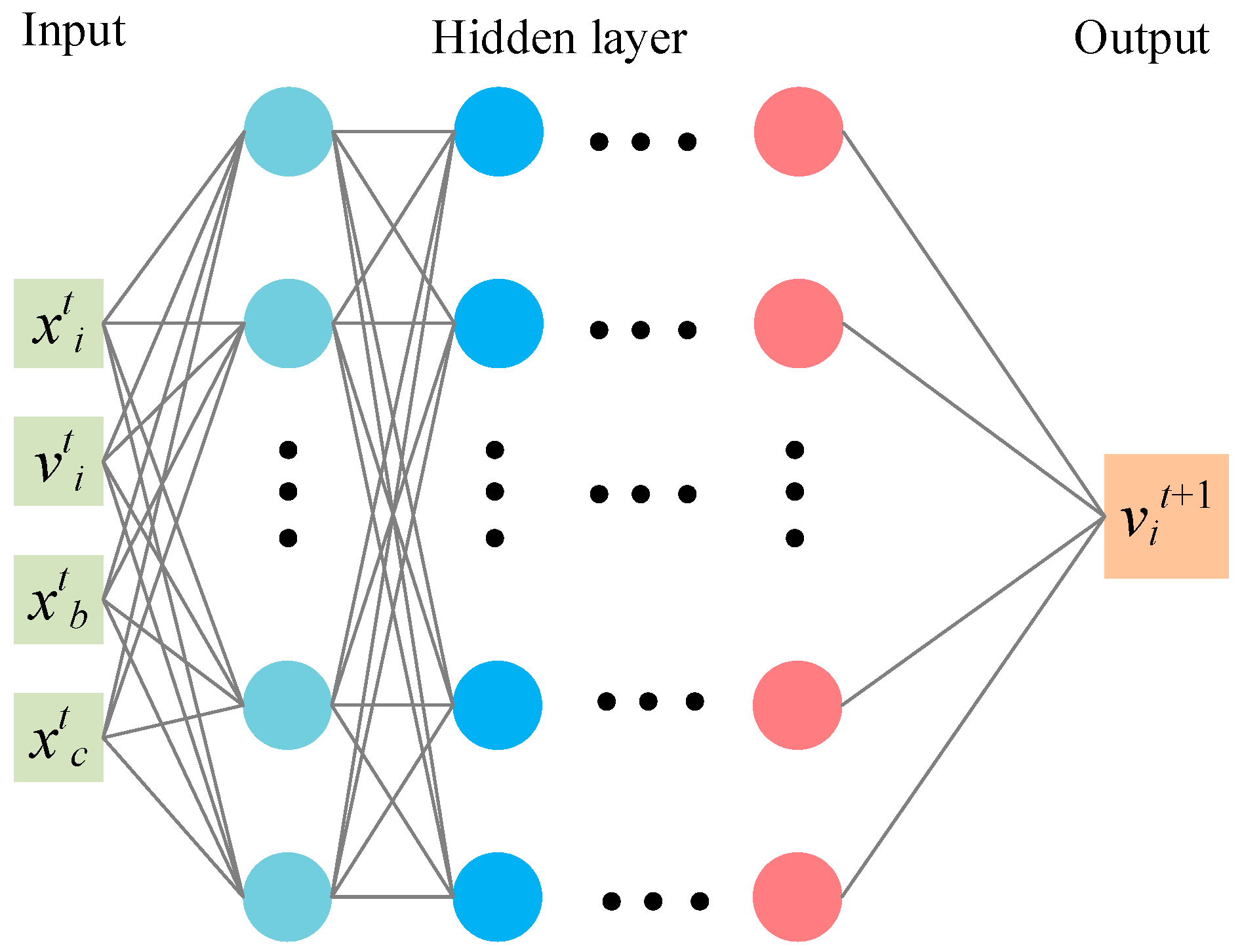
To further improve the identification accuracy of the SGA and to avoid premature convergence to local optima, a policy network π_θ(·) is introduced to replace the traditional velocity update formula of the standard SGA. The network takes as input the current position of the individual, the current velocity, the current global best position, and the current global center position. It outputs the updated velocity for the next iteration. As shown in Figure 2, a fully connected neural network is designed to capture the nonlinear relationship between the input features and the updated velocity. The neural network structure (4-30-30-30-30-30-1) comprises five hidden layers, offering sufficient depth to model complex dynamics during the optimization process.

The state vector is constructed for each individual, representing its status at the t-th iteration. The state vector for an individual at iteration t is defined as:

$$s_i^t=[x_i^t,v_i^t,x_b^t,x_c^t]\in R^{4D}$$

(17)

where:

$x_i^t$ represents the current estimated kinematic parameter error of the individual,

$v_i^t$ denotes the current adjustment velocity, corresponding to the step size and direction of parameter correction,

$x_b^t$ refers to the current global best estimated kinematic parameter error among all individuals, serving as the best-known calibration solution so far,

$x_c^t$ is the current global center position of the population, reflecting the collective search status.

The policy network takes this state vector as input and outputs a new adjustment velocity $v_{t+1}^i$. This predicted velocity represents the next movement direction and step size for updating the estimated kinematic parameters, aiming to minimize the overall calibration residuals. The policy network is defined as:

$$v_i^{t+1}={\pi }_{\theta }(s_i^t)$$

(18)

The output v_i^t+1 corresponds to the velocity update for the next iteration.

The training objective of the policy network is formulated as a supervised learning task. Training samples ($S_i^t$, v_i^t+1) are collected by observing the actual behavior of the standard SGA. The loss function is defined as:

$$\mathcal{l}(\theta )={\displaystyle \frac{1}{M}}{\displaystyle \sum _{i=1}^M‖{\pi }_{\theta }(S_i^t-v_i^{t+1})‖}$$

(19)

where M denotes the number of training samples.

In the context of robot calibration, the input state vector elements correspond to the estimated kinematic parameter deviations and their dynamic adjustment behaviors, while the output velocity adjustment guides the refinement of the calibration parameter estimates to achieve higher positioning accuracy.

The position update is performed using the updated velocity according to the following formula:

$$x_i^{t+1}=x_i^t+v_i^{t+1}+{\Delta }_{mig}^t$$

(20)

where ${\Delta }_{mig}^t$ is a perturbation term derived from the modeling of snow geese migration behavior, including V-formation, linear flight, and Brownian motion.

$${\Delta }_{mig}^t=\left\{\begin{array}{l}a(x_b^t-x_i^t)+b(x_c^t-x_i^t),\\ (x_i^t-x_b^t)\cdot \gamma ,\\ (x_i^t-x_b^t)\cdot \gamma \oplus Brownian(\dim ),\end{array}\right.\begin{array}{c}\theta <\pi \\ \gamma >0.5\\ \gamma \le 0.5\end{array}$$

(21)

A convergence-checking mechanism was incorporated into the RLSGA implementation, where convergence is confirmed based on objective function improvement thresholds, and a convergence alarm is triggered if the convergence condition is not satisfied within the maximum allowable iterations.

In each iteration, the state vector of each agent is processed by the policy network to infer the new adjustment velocity, which is subsequently combined with SGA migration updates for position refinement. The updated position is then evaluated for calibration accuracy, completing one cycle of interaction between the learning and optimization components.

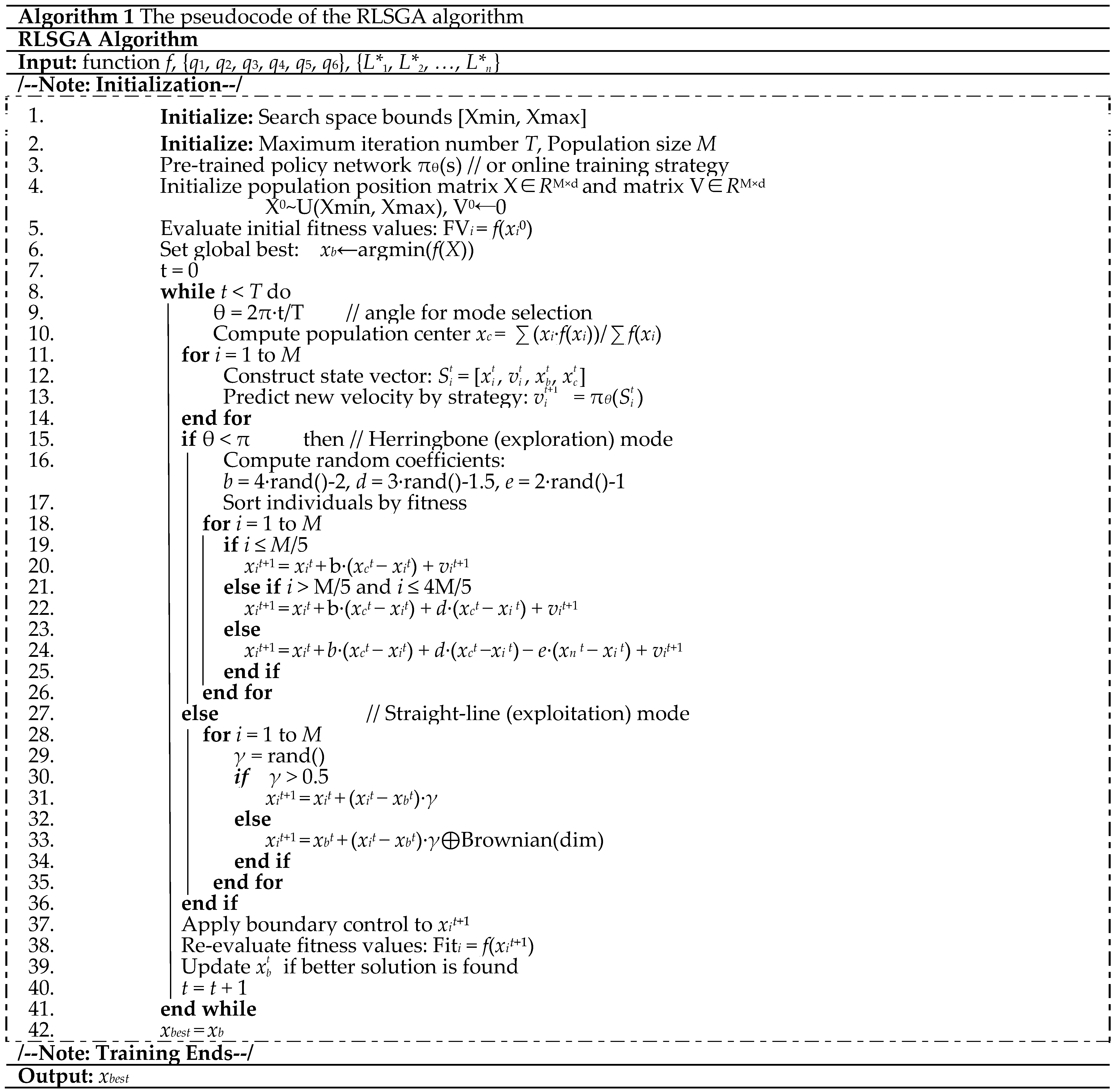
Algorithm 1 presents the pseudo-code of the proposed RLSGA algorithm for solving the robot calibration problem. RLSGA builds upon the conventional SGA by integrating a deep policy network to model individual migration behaviors adaptively. Instead of relying on fixed-velocity update formulas, the algorithm leverages learned state-action mappings to predict individual movement directions, thereby enhancing its adaptability and convergence efficiency in high-dimensional and nonlinear optimization scenarios. Meanwhile, the inherent biological behaviors of SGA—namely, the V-formation and straight-line flight—are preserved and combined with the learned strategy to form a collaborative search mechanism. This hybrid approach makes SGA-RL particularly suitable for complex robot calibration tasks involving multi-source uncertainties and nonlinear parameter dependencies.

Unlike conventional gradient-based methods that require explicit Jacobian and Hessian computations, the proposed RLSGA operates through population-based stochastic updates guided by a deep policy network, thereby avoiding numerical instabilities associated with near-singular configurations and heterogeneous constraint conditions.

3.3. Performance Evaluation of RLSGA

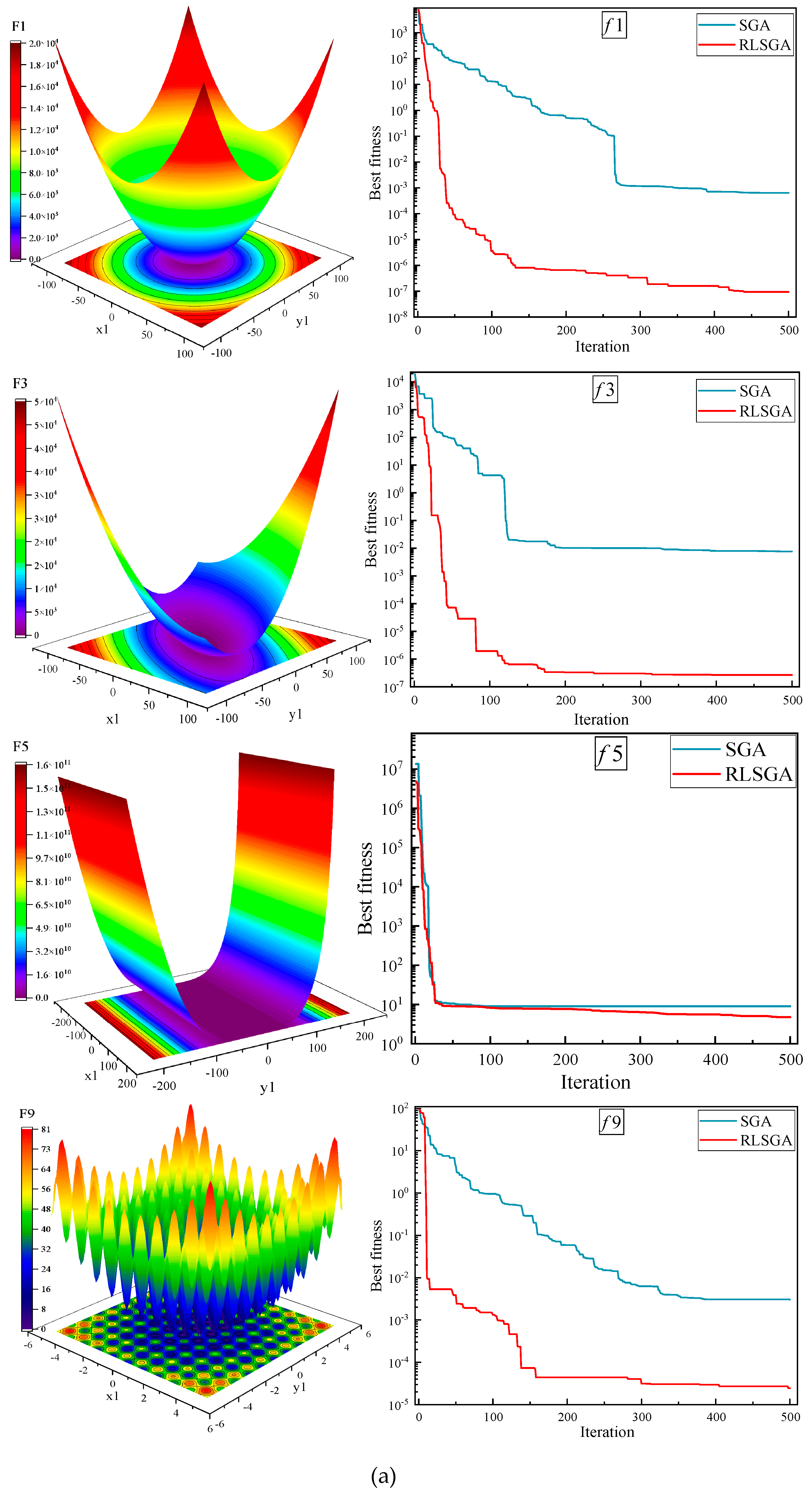
To validate the performance improvement introduced by RLSGA, several representative benchmark functions (f1, f3, f5, f9, f13, f15, f16, f20, f22) from the CEC2005 test suite are selected for evaluation. The original SGA is used as a baseline for comparison. Figure 3 presents the experimental results, illustrating the convergence behavior of both algorithms across the selected test functions. As shown in Figure 3, the improved RLSGA demonstrates significantly better performance than the original SGA in terms of both convergence speed and solution accuracy. Specifically, RLSGA converges faster and reaches lower final objective values on most functions, indicating its superior optimization capability. These results confirm the effectiveness of incorporating deep reinforcement learning into the optimization process. The learning-guided strategy enables RLSGA to dynamically adapt its search direction, enhancing global exploration and local exploitation abilities in complex, high-dimensional search spaces.

4. Robot Kinematic Calibration Experiment

4.1. Experimental Conditions

4.1.1. Experimental Platform and Data Acquisition

An experimental platform, depicted in Figure 4, is constructed to enable high-precision calibration of the robot. The setup consists of an ABB IRB120 industrial robotic arm, featuring a repeatability of 0.01 mm, along with a cable-type displacement sensor, a digital displacement display unit, and an RS485 communication interface. This configuration ensures accurate displacement acquisition and stable data transmission during the calibration process.

Table 2. Specifications of the drawstring displacement sensor.

Parameter	Value
Measuring range	2000 mm
Maximum operating speed	1000 m/s
Retraction force	5 N
Measurement resolution	0.004 mm
Operating temperature range	−25 °C~+85 °C

provides detailed specifications of the drawstring displacement sensor.

To ensure the accuracy and representativeness of the calibration dataset, measurement points were comprehensively distributed across the entire operational workspace of the ABB IRB120 industrial robot. A total of 1042 measurement positions were strategically selected, and their spatial coordinates were captured using a high-resolution drawstring (cable-type) displacement sensor with a resolution of 0.004 mm. To facilitate efficient and consistent data recording, a customized acquisition program was developed using LabVIEW software, enabling the automated logging of sample information. To mitigate potential ill-posedness caused by degenerate configurations, the measurement points were carefully distributed across the entire reachable workspace of the robot, covering diverse joint configurations and spatial locations. This ensures sufficient excitation of all degrees of freedom during calibration.

From the collected measurement data, 200 representative samples were randomly selected under a uniform distribution to construct each calibration case. To mitigate the potential effects of sampling bias and improve statistical robustness, the random selection process was repeated 10 times, resulting in 10 distinct calibration data cases. In each case, the selected dataset was divided into two subsets: 160 samples (80%) were allocated for training purposes to fit the calibration models, while the remaining 40 samples (20%) were reserved for independent testing to evaluate generalization capability. This consistent partitioning strategy facilitates a balanced assessment of both model accuracy and robustness across different data scenarios. During model evaluation, each method’s calibration performance was assessed separately on these 10 data cases. The final reported results, including RMSE, Std, and Max positioning errors, represent the mean and standard deviation across all 10 cases, thereby ensuring that the evaluation is statistically reliable and not dependent on a specific sampling instance.

Furthermore, to support transparency and encourage reproducibility, the resulting dataset, along with detailed documentation, has been made publicly available at https://github.com/Lizhibing1490183152/RobotCali (accessed on 1 August 2022), providing a reliable benchmark for further research in robot calibration studies.

4.1.2. Evaluation Metrics and Comparison Methods

In the context of large-scale industrial applications, a primary objective of robot calibration is to enhance the robot’s absolute positioning accuracy, thereby meeting the stringent demands of high-precision manufacturing processes [7,8,9,10]. To comprehensively assess the effectiveness of the calibration method, three widely recognized statistical indicators are employed as performance metrics: root mean squared error (RMSE), standard deviation (Std), and maximum error (Max). These metrics provide insights into the overall positioning precision, consistency, and worst-case deviations of the robotic system. The mathematical definitions of these evaluation indicators are formulated as follows:

$$\begin{array}{l}Max=\max \left\{\sqrt{{(L_i-{L_i}^{*})}^2}\right\},i=1,2,\cdots ,m\\ Std={\displaystyle \frac{1}{m}}{\displaystyle \sum _{i=1}^m\sqrt{{(L_i-{L_i}^{*})}^2}}\\ RMSE=\sqrt{{\displaystyle \frac{1}{m}}{\displaystyle \sum _{i=1}^m{(L_i-{L_i}^{*})}^2}}\end{array}$$

(22)

To validate the effectiveness and superiority of the proposed calibration approach, a series of comparative experiments were conducted against several representative state-of-the-art methods. These benchmark techniques are selected based on their relevance and proven performance in the field of robot kinematic calibration. The specific comparative strategies and experimental settings are outlined as follows, aiming to ensure a fair and comprehensive evaluation of calibration accuracy across different algorithms.

M1: The extended Kalman filter (EKF) algorithm, as introduced in [8], is capable of effectively handling non-Gaussian noise within the calibration framework.

M2: An LM-based calibration model [7], widely used in practice, optimizes the calibration objective by minimizing the residual gradient to identify D-H parameters.

M3: The particle swarm optimization (PSO) algorithm [17] mimics the flocking behavior of birds to efficiently search for optimal solutions.

M4: The differential evolution (DE) algorithm [18] is a population-based optimization method capable of performing accurate multi-objective robot calibration.

M5: The beetle antennae search (BAS) algorithm [13] emulates the foraging mechanism of beetles to solve complex optimization tasks.

M6: The artificial bee colony (ABC) [11] algorithm is employed for calibrating the D-H parameters of industrial robots.

M7: The snow geese algorithm (SGA) [16,19], inspired by the flocking behavior of snow geese, is utilized for calibrating the robot’s kinematic parameters.

M8: The proposed method, a deep reinforcement learning-enhanced snow geese algorithm (RLSGA), is applied to robot calibration to further improve the accuracy of parameter identification.

Table 3. Hyper-parameter settings.

Method	Hyper Parameter
M1	Pk = 0.5 × 10−7, Qk = 0.5 × 10−7, Rk = 0.2 × 10−4
M2	μ = 0.5 × 10−3
M3	M = 100, c1 = 1.2, c2 = 1.2, ω = 0.8
M4	M = 100, F = 0.5, CR = 0.1
M5	d0 = 0.01, δ0 = 0.01, eta = 0.95
M6	M = 100, Eb = 50, Ob = 25, limit = 1000
M7	M = 100, L = 10, α = 0.2, β = 0.05
M8	M = 100, L = 10, α = 0.2, β = 0.05, lr = 0.005, γ = 0.9, ε = 0.9, network structure (4-30-30-30-30-30-1)

presents the hyperparameter configurations that yielded the best calibration performance for each model during the tuning process. Each setting was determined based on extensive empirical evaluation, aiming to maximize the accuracy and robustness of the respective optimization strategies.

4.2. Experimental Results

Figure 5, Figure 6 and Figure 7 present, respectively, the calibration effectiveness, the positioning accuracy, and the convergence trends achieved by models M1 through M8.

Table 4. Comparison of calibration results.

Item	RMSE (mm)	STD (mm)	Max (mm)	Time (s)
Before	2.263	2.131	3.876	/
M1	0.652	0.553	1.685	80.321
M2	0.511	0.446	1.235	70.348
M3	0.625	0.52	1.467	135.982
M4	0.667	0.592	1.721	95.351
M5	0.701	0.622	1.851	134.761
M6	0.585	0.498	1.401	110.917
M7	0.544	0.467	1.328	100.648
M8	0.481	0.408	1.002	150.327

summarizes the comparative calibration results, including the overall time consumption associated with each evaluated method. Furthermore, the optimized D-H parameter compensation values obtained through M8, namely, the proposed RLSGA approach, are detailed in

Table 5. Calibrated kinematic parameters of the ABB IRB120 robot.

Joint i	αi/Degree	ai/mm	di/mm	θi/Degree
1	−90.214	0.175	292.375	2.176
2	0.0347	273.847	0.728	−90.758
3	−91.387	73.695	−0.743	0.016
4	88.367	0.671	302.684	0.748
5	−90.476	0.058	−1.736	−3.753
6	0.176	1.278	72.247	1.274

.

Based on these experimental outcomes, several noteworthy observations can be made:

The proposed RLSGA algorithm (M8) achieves effective calibration results for the robot system. Table 4 and Figure 5 present the calibration performance before and after applying the optimization strategy. M8 exhibits significant improvements across all evaluation metrics when compared to the uncalibrated condition. Specifically, M8 reduces the RMSE from 2.263 mm to 0.481 mm, the Std from 2.131 mm to 0.408 mm, and the Max from 3.876 mm to 1.002 mm, corresponding to improvements of 78.75%, 80.85%, and 74.15%, respectively.

M8 exhibits the best overall performance in terms of robot calibration accuracy, compared with M1 to M7. As reported in Table 4 and Figure 5, the RMSE, Std, and Max obtained by M8 are 0.481 mm, 0.408 mm, and 1.002 mm, respectively. Taking M2, the most accurate among the baseline methods, as a comparison point, its corresponding RMSE, Std, and Max are 0.511 mm, 0.446 mm, and 1.235 mm, respectively. On this basis, M8 achieves accuracy improvements of 5.87%, 8.52%, and 18.87%, respectively, in the three metrics. These findings confirm that the proposed RLSGA approach delivers notable enhancements in accuracy and is thus effective in improving robot calibration performance.

M8 is an enhanced version of the standard SGA algorithm (M7), incorporating deep reinforcement learning to guide the optimization process. Compared to M7, M8 achieves notable improvements in calibration accuracy. Specifically, as shown in Table 2 and Figure 5, M8 reduces the RMSE from 0.544 mm to 0.481 mm (an 11.58% improvement), the Std from 0.467 mm to 0.408 mm (12.63% improvement), and the Max from 1.328 mm to 1.002 mm, yielding a significant 24.55% reduction. These results demonstrate that integrating a deep policy network into the SGA framework can effectively enhance optimization behavior, leading to better calibration accuracy. The proposed RLSGA outperforms its base version (SGA), verifying the effectiveness of reinforcement learning in guiding population-based evolutionary strategies.

In addition to calibration accuracy, the computational cost is an important factor when evaluating the overall performance of optimization algorithms. As shown in Table 2 and Figure 5, M8 (RLSGA) exhibits the longest execution time of 150.327 s, which is higher than all the baseline methods (M1–M7). This increased time consumption is primarily attributed to the additional training and inference processes involved in the deep reinforcement learning strategy embedded in RLSGA. For example, M8 requires approximately 49.7% more time than M6 (100.648 s) and nearly doubles the runtime compared to M2 (70.348 s), which was the fastest among all tested methods. While M8 achieves the best calibration accuracy across all evaluation metrics, these results also reveal a trade-off between optimization precision and computational efficiency. Nevertheless, such a cost is acceptable and often worthwhile in applications where accuracy is of paramount importance.

Figure 6 illustrates the convergence behavior of different calibration methods in terms of RMSE-position error over 60 iterations. It is evident that M8 (RLSGA) consistently outperforms the other methods in both convergence speed and final accuracy. In the top subfigure, which compares M1, M3, M5, M7, and M8, the M8 curve exhibits a steep decline in the early iterations and quickly converges to a lower RMSE level than its counterparts. While M1 and M5 plateau at relatively higher error levels, M8 continues to descend and stabilizes with minimal fluctuations. Notably, M7 (the original SGA) converges more slowly and reaches a higher final RMSE than M8, highlighting the effectiveness of introducing deep reinforcement learning in RLSGA. Similarly, in the bottom subfigure comparing M2, M4, M6, and M8, M8 again achieves the fastest and smoothest convergence trajectory. Although M2 and M6 initially decline rapidly, their curves plateau earlier and settle at higher error levels compared to M8. These results demonstrate that M8 not only reaches the lowest final RMSE but also exhibits superior convergence characteristics, validating the advantage of the proposed method in both optimization capability and learning efficiency during calibration.

A total of 200 measurement points were collected using an ABB IRB120 industrial robot. Upon completing the calibration process for these measurement points, the resulting positioning accuracy of each method is evaluated and compared, as presented in Figure 7. Figure 7 illustrates the calibrated position errors of different methods across all measurement points. Each horizontal group of markers corresponds to a specific calibration method, where the distribution of points reflects the residual positioning error for the test samples. It can be observed that before calibration (black squares), the positioning errors are significantly larger and more dispersed, often exceeding 2 mm. After calibration, all methods (M1–M8) substantially reduce the error magnitude. Among them, M8 (the proposed RLSGA method, red stars) exhibits the lowest and most concentrated residual error distribution. The error points of M8 consistently remain below 1.0 mm, with most residuals clustered around 0.4–0.6 mm. In contrast, other methods such as M1, M3, and M5 show wider scatter and larger error magnitudes, indicating less stable calibration performance. Furthermore, the dashed lines representing the RMSE values clearly indicate that M8 achieves the lowest RMSE among all methods. Specifically, the horizontal dashed line for M8 is located lower than those for M1–M7, validating the superior positioning accuracy and consistency of the proposed method. Notably, while M7 (SGA) performs reasonably well, its residual distribution is still broader compared to M8, emphasizing the benefits brought by integrating deep reinforcement learning into the optimization framework. These observations from Figure 7 strongly confirm that the proposed RLSGA method (M8) not only minimizes the overall positioning error but also ensures better consistency across different measurement points, thus demonstrating its effectiveness in improving the absolute positioning accuracy of industrial robots.

5. Conclusions

To enhance the calibration accuracy of industrial robots, this paper proposed a novel RLSGA algorithm, which integrates deep reinforcement learning with a biologically inspired metaheuristic framework. A series of benchmark function tests and robot calibration experiments were conducted to verify the effectiveness and superiority of the proposed method. The main conclusions are summarized as follows:

(1) In comparison with the original SGA, the proposed RLSGA demonstrates significantly improved performance on the CEC2005 benchmark functions in terms of convergence speed and solution accuracy. By introducing a learned policy network to adaptively guide the optimization process, RLSGA effectively overcomes the limitations of premature convergence and local optima, enhancing both global exploration and local exploitation capabilities.

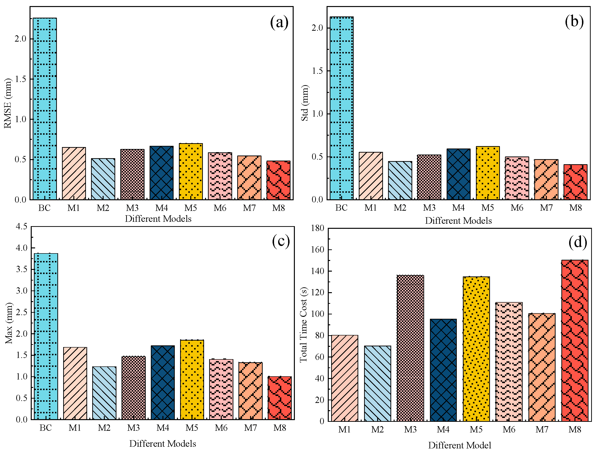
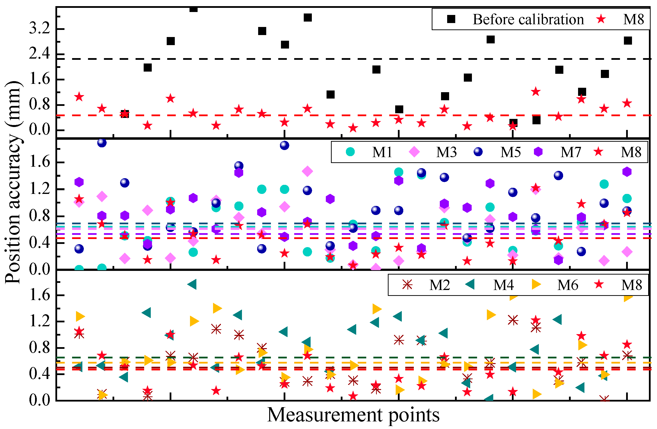
(2) In industrial robot calibration tasks, RLSGA achieves the highest calibration accuracy among eight representative methods, including both classical optimization algorithms (e.g., PSO, DE) and advanced heuristics (e.g., BAS, ABC). Specifically, RLSGA reduces the RMSE, Std, and Max to 0.481 mm, 0.408 mm, and 1.002 mm, respectively, representing the best performance across all evaluated metrics. Moreover, its convergence curves are smoother and faster than those of the baseline methods, confirming the robustness and learning efficiency of the proposed strategy.

(3) Although RLSGA incurs higher computational cost due to the training and inference procedures of the deep policy network, this trade-off is acceptable in high-precision applications where calibration accuracy is of critical importance. Overall, the proposed RLSGA provides a promising solution for robot calibration tasks with complex, nonlinear error models and offers potential for broader applications in intelligent manufacturing and adaptive robotics.

In future work, several promising research directions can be explored to further enhance the effectiveness and applicability of the proposed RLSGA method. First, developing online learning strategies could enable real-time adaptation of the calibration model during robot operation, improving dynamic accuracy under changing conditions. Second, extending the kinematic error modeling to incorporate thermal effects, payload variations, and other environmental factors could further improve calibration robustness. Third, applying the RLSGA framework to different types of robots, such as collaborative or redundant robots, would validate its generalization capability across various robotic platforms. These potential extensions will be the focus of our subsequent research.