Abstract
Selecting grid loss reduction strategies is crucial for energy-saving transformations, particularly in the context of electricity transmission and distribution pricing reforms. The optimization of strategic selection is not easy due to the vast number of grid devices, which leads to a multitude of possible strategy combinations. This paper presents an optimal model for selecting loss reduction strategies, aiming to minimize the sum of comprehensive investment costs and energy loss costs over the life cycle of the strategies. The energy loss costs include both direct expenses due to energy loss and indirect costs, namely, carbon emission penalties. The constraints include allowable voltage deviations, branch power transmission, the number of loss reduction measures, loss rates, and total investment limits. The model comprehensively considers both economic benefits and the social benefits of reduced carbon emissions. It can help companies better adapt to electricity transmission and distribution pricing reforms, reduce operational costs, and contribute to low-carbon development. Finally, the model is validated using the data provided by one provincial power grid company in China. The results show that the loss reduction reaches 13.9 MW and the reduced carbon emission per hour is 10.425 t. The proposed method is also compared with the enumeration method, which demonstrates its effectiveness and efficiency. Further research will be conducted on establishing functional relationships between electricity sales prices and line losses to incentivize companies to apply loss reduction measures under different pricing functions.
1. Introduction
The power system, as an essential infrastructure of modern society, plays a pivotal role in the stable development of the economy and the sustainability of the environment [1]. The transmission and distribution segment, being a critical part of the power system, directly impacts energy utilization efficiency and electricity costs through its energy consumption and losses [2]. Therefore, investigating energy-saving and loss reduction strategies within the framework of electricity transmission and distribution pricing mechanisms is of significant importance for enhancing the energy efficiency of the entire power system, reducing operational costs, and promoting green and low-carbon development.
Currently, the energy-saving transformation of distribution networks is a comprehensive engineering task that includes equipment upgrades, grid structure optimization, network reconfiguration, reactive power compensation, and operational enhancements [3]. Extensive research has been conducted both domestically and internationally on loss reduction and energy-saving strategies for distribution networks [4]. Devices such as shunt capacitors and reactors, known for their cost effectiveness and practicality, have become key tools for energy conservation and loss reduction [5]. For example, Li and Xu [6] explored the use of high-voltage single-phase power supply methods, while Long et al. [7] focused on energy-efficient distribution transformers. There are also researchers who have investigated loss reduction strategies for low-voltage and medium-voltage distribution networks, respectively [8,9].
In the context of global climate change and the urgent need to reduce greenhouse gas emissions, the energy sector, particularly the electricity industry, is under immense pressure to transition towards cleaner and more sustainable practices [10]. The integration of renewable energy sources, while beneficial for reducing carbon emissions, also introduces new challenges for grid management due to their intermittent and variable nature [11]. This complexity necessitates advanced strategies for grid loss reduction that can adapt to the dynamic changes in power generation and consumption patterns.
With the advancement of technology, an increasing array of methods is available for energy conservation and carbon reduction. For instance, in the context of power grids, energy-saving modifications can be implemented through various means, including the transformation of wire cross-sections, the optimization of power supply radii, and the redistribution of electrical loads. Moreover, given the vast number of grid devices, the resulting combinations of strategies are numerous, making the optimization of strategic selection a critical issue. Evidently, the selection of grid loss reduction strategies can lead to different outcomes in terms of both economic and environmental performance [12]. Against this backdrop, this paper proposes an optimization model for selecting grid loss reduction strategies that not only minimizes the sum of comprehensive investment costs and energy loss costs over the life cycle of the strategies but also considers the indirect costs associated with carbon emissions. The model is designed to be flexible and adaptable to various scenarios, allowing for the inclusion of constraints on the number of loss reduction measures and total investment limits.
The main novelty of this article lies in the development of an optimization model that comprehensively considers both economic and environmental factors in grid loss reduction strategies. Specifically, the model includes:
- (1)
- The model accounts for indirect costs associated with carbon emissions, providing a more comprehensive evaluation of the economic and environmental impacts of different loss reduction strategies.
- (2)
- This study employs an adaptive genetic algorithm to solve the optimization problem, which is more efficient and effective than traditional enumeration methods, especially when dealing with a large number of possible strategy combinations.
- (3)
- The model is validated using data from a provincial power grid company in China, demonstrating its practical applicability and effectiveness in reducing grid losses and carbon emissions.
The remainder of this paper is structured as follows: Section 2 provides a literature review of the current state of research on grid loss reduction strategies and optimization models. Section 3 details the methods and analysis used in this study, including the formulation of the objective function and constraints, as well as the optimization approach. Section 4 presents the results of this case study and the application of the proposed method to a provincial power grid company in China. Section 5 discusses the potential synergies with renewable energy sources and technologies, as well as economic concerns related to the proposed method. Finally, Section 5 concludes this paper and suggests directions for future research.
2. Literature Review
Researchers are continuously deepening their research on the construction of loss reduction methods for distribution networks. Xie et al. [13] proposed a combined power loss reduction strategy optimization framework for distribution networks, which analyzes weak points through power flow calculations and generates strategies involving conductor replacement, transformer upgrading, and reactive power compensation. Wang et al. [14] examined the EZ Power Grid to identify common issues in current power grids and proposes methods for evaluating power loss reduction. Suresh and Edward [15] established a hybrid optimization technique combining the Grasshopper Optimization Algorithm (GOA) and Cuckoo Search (CS) to determine the optimal placement and sizing of distributed generation (DG) units in electric power networks, aiming to reduce power losses, improve voltage profiles, and enhance system reliability. Pokhrel et al. [16] proposed a mixed loss optimization problem that considers network reconstruction, distributed generation and distributed storage, and solved it using the interior point method. Ahmadi et al. [17] proposed an efficient power loss reduction (briefly, PLR) model based on four PLR schemes: distributed generation installation, distribution network reconstruction, capacitor bank installation, and distribution feeder reinforcement. The proposed PLR strategy incorporates budget constraints as a hard constraint for distribution network planning. Iweh et al. [18] comprehensively reviews the integration of distributed generation, particularly renewable energy sources, into the power grid, discussing the prerequisites, push factors, practical options, challenges, and merits of such integration. Similar studies can be found in [19,20]. Mu et al. [21] employs a two-stage power optimization model to analyze the potential of Carbon Capture, Utilization, and Storage (CCUS) in achieving carbon neutrality in China’s Northeast Power Grid. However, none of these research studies provided solutions on selecting and combining different strategies to derive the optimal loss reduction method.
There are also researchers who focus on the study of optimization strategies for loss reduction schemes in distribution networks. Zhang et al. [22] introduced a model-free volt-VAR optimization algorithm using multi-agent deep reinforcement learning (DRL) for unbalanced distribution systems, employing a deep Q-network (DQN) framework to intelligently manage voltage regulation and power loss reduction without directly solving a specific optimization model. Zhang et al. [23] proposed an improved genetic algorithm for power distribution system reconfiguration based on Sandeep Sehgal’s research, which reduces the number of switching operations and improves system reliability [24]. Gautam and Bhusal [25] proposed a genetic algorithm based on spanning tree to optimize distribution system reconfiguration. This algorithm filters the invalid configuration combinations in the selection process of genetic algorithm, reduces the dimension of the search space of genetic algorithm, and has higher accuracy and efficiency. Kamel et al. [26] proposed a new optimization technique (SSA) to reduce the total active power loss. With parallel optimization and search functions, SSA is an effective technology for radial distribution network reconfiguration. Wu et al. [27] proposed an optimization strategy based on the combat strategy algorithm for the randomness and load uncertainty of distributed generation. This method significantly reduced the overall line loss of distribution network during the peak load period. However, these articles only consider the direct losses caused by electricity waste, and they do not provide a detailed calculation of the losses due to carbon dioxide penalties; hence, the conclusions are not comprehensive.
To sum up, despite extensive research on grid loss reduction strategies and optimization models, the existing studies often focus on singular approaches to loss reduction and lack systematic optimization for strategy combinations. Additionally, there is a scarcity of research on models that prioritize loss reduction strategies while considering the benefits of low-carbon emissions. Most prior studies either neglect the indirect costs associated with carbon emissions or fail to provide comprehensive optimization frameworks that integrate both economic and environmental factors. This gap is particularly evident in the context of electricity transmission and distribution pricing reforms, where a holistic approach to grid loss reduction is urgently needed.
3. Methods and Analysis
The loss reduction model is this study seeks to minimize the total costs, which include both the comprehensive investment expenses and the electrical energy loss expenses, over the entire lifespan of the loss reduction strategy. The electrical energy loss expenses encompass direct costs and indirect costs, notably, the penalties associated with carbon emissions. The model is subject to several constraints, including the permissible voltage deviation in the lines, the transmission power (current) of the branches, the number of loss reduction measures, the rate of energy loss, and the limit on the total allowable investment.
3.1. Objective Function
Considering that direct and indirect costs are both calculated on an annual basis, investment costs must also be converted into average annual investment costs. With a 10-year investment cycle, the objective function to be optimized in this paper is shown in Equation (1):
In this function, is comprehensive investment from ith loss-reduction measures; is the total number of loss reduction measures; is the direct cost caused by the loss of electricity, referring to the loss of electricity caused by the loss of electricity; is the indirect cost caused by the loss of electricity, which refers to the carbon emission penalty caused by the loss of electricity. All these components can be calculated by Equations (2)–(7).
- (1)
- Comprehensive investment for loss-reduction measures :
The comprehensive investment for loss reduction measures includes equipment acquisition , equipment removal and installation or reconstruction [13]. The function is:
- (2)
- Direct cost due to loss of electricity :
The direct cost caused by the loss of electricity is also known as the power loss cost [13]. The function is:
In this equation, refers to power loss, kW·h; is electricity price, generally CNY 0.5 per kW·h.
- (3)
- Indirect cost due to loss of electricity :
The indirect cost of lost electricity, i.e., the carbon (CO2) emission penalty, can be calculated by [28]:
In the equation, refers to the carbon (CO2) emission penalty per unit of electricity generation [13], which is calculated by:
In the above equation, is the proportion of thermal power; in China, the number is around 65%; is the carbon penalty [13,15]; is carbon (CO2) emissions per unit of electricity generation, kg/(kW·h), and the equation of Q is [29]:
In the above equation, p refers to carbon emissions per unit (per ton) of fuel, 2.53 kg CO2/kgCoal [15]; is heat output per ton of fuel [13,15]; and the calorific value of coal per kilogram of fuel is 6400 kcal/kg Coal = 6400 × 4.185 8 = 26,789.12 kJ/kgCoal = 26.789 kJ/t [19]; is the energy conversion rate of a power source [15]; 1 W·s = 1 J, 1 kW·h = 3600 kJ. Considering the thermal efficiency of a coal fired power plant, is set to be 0.4 kW·h/3600 kJ. The quotation follows Equation (7):
According to our carbon emission penalty standard, the price is set at 0.2 CNY/kg [16], . Based on the European Union’s penalty standards for carbon emissions during 2008–2012 (100 EUR/t ), = 0.1 EUR/kg ≈ 0.733 CNY/kg. As a result, CNY/(kW·h).
3.2. Constraint
The constraints include voltage deviation, branch constraints, quantitative restriction of loss reduction and the total investment limit.
- (1)
- The voltage deviation is [30]:
In this equation, is the actual voltage of node , kV; is the rated voltage, kV.
The allowable voltage deviation [18] in the 10 kV voltage class does not exceed:
- (2)
- Branch constraints. The actual transmission capacity of the branch shall not exceed its maximum transmission capacity, expressed by the transmission current [30]:
In this inequation, is the actual current of branch ; is the maximum current allowed through branch .
- (3)
- The quantitative restriction of loss reduction measures is:
In this inequation, refers to the maximum number of loss reduction measures.
- (4)
- The total investment limit is:
In the above inequation, is the limit of total investment, the unit is ten thousand.
Notations related the parameters occurred in the above equations are summarized in Table 1.

Table 1.
Notations.
3.3. Optimization
According to the principle that one loss reduction measure can constitute a loss reduction plan, and the combination of one or several loss reduction measures can also constitute a loss reduction plan, the decision variable (0 or 1) is whether each loss reduction measure is implemented or not. Assuming that there are loss reduction measures, there will be loss reduction schemes, and the solving process is a combinatorial optimization problem. The genetic algorithm has strong searching ability and low dependence on objective function; so, it is very suitable for solving such problems. The adaptive genetic algorithm (briefly, AGA) was proposed by Srinivas [31], which adjusts the crossover rate and variation rate according to the fitness value of the progeny population after each iteration. Compared with the standard genetic algorithm (SGA), it has better convergence speed. Compared with other algorithms, such as particle swarm optimization (PSO), the AGA dynamically adjusts mutation and crossover rates to maintain population diversity, avoiding premature convergence. This allows the AGA to perform broad searches early for diversity and fine searches later to protect optimal solutions, leading to more effective convergence to the global optimum [32]. Additionally, the AGA naturally handles discrete variables, such as binary encoding, while PSO, designed for continuous spaces, struggles with discrete combinatorial optimization problems and requires additional modifications [33]. Moreover, in high-dimensional or non-convex problems, PSO may fail due to particle trajectory divergence and is prone to local optima [34]. The AGA enhances stability through increased mutation rates to introduce new solutions and employs divide-and-conquer strategies like variable grouping to reduce problem coupling, making it more effective for complex optimization tasks.
The overall flow of loss reduction scheme optimization is shown in Figure 1.
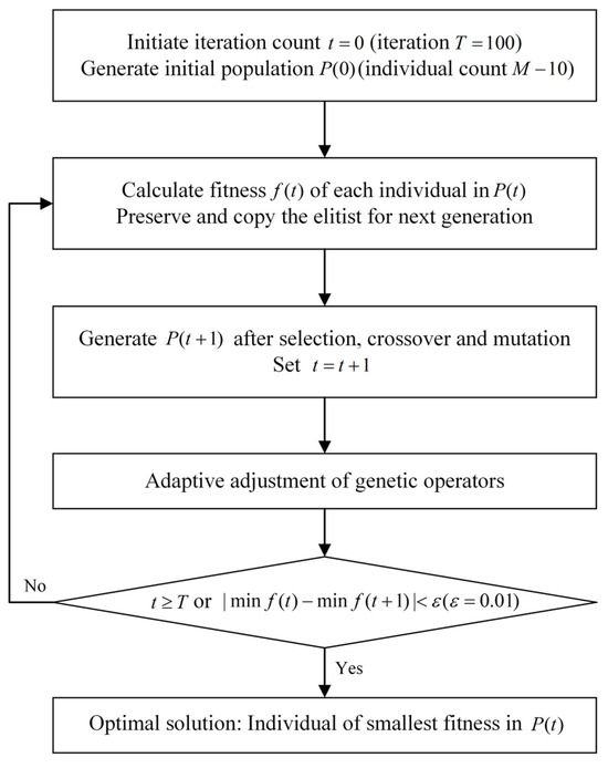
Figure 1.
Flowchart of main steps of the adaptive genetic algorithm.
- (1)
- Encoding
If the genetic algorithm is used, the problem needs to be encoded first. The implementation of each loss reduction measure corresponds to 1 bit of binary code (0 or 1, called gene); so, the binary code can be used to describe each loss reduction plan. The length of the binary code of the loss reduction scheme is set according to the number of loss reduction measures. If the number of loss reduction measures is n, it is set as a n-bit binary code.
- (2)
- Fitness function
In this paper, constraint conditions are combined into the fitness function to achieve a fitness function with a penalty term, which can guide genetic search. And the fitness function is:
In the equation, , , and are penalty factors, which are all set to be 1. is 0-1 function, which is defined as follows:
- (3)
- Genetic manipulation
Calculate the fitness value of each individual in the population ; the optimal individual is retained, and the current optimal individual is copied directly to the next generation.
- (1)
- Adaptive cross operation
In the iterative process of the SGA, crossover probability and mutation probability are fixed. However, the AGA calculated the probabilities of crossover and mutation depending on the fitness values of the solutions. High-fitness solutions are kept, while solutions with subaverage fitness are totally disrupted. According to the fitness value of progeny population, the dynamic adjustment crossover rate of the adaptive genetic algorithm is:
where is the population maximum fitness; is the larger fitness among the two individuals involved in the crossover; is the average fitness of the population. and are the maximum and minimum crossing probabilities, respectively.
- (2)
- Mutation operation
The adaptive genetic algorithm dynamically adjusts the mutation probability according to the fitness value of the offspring population.
where is the fitness of the mutated individual. and are the maximum and minimum mutation probabilities, respectively.
- (4)
- Iterative termination condition
The condition of setting iterative convergence: meet one of the following iterative convergence conditions.
- (1)
- The number of iterations has reached the maximum number of iterations M;
- (2)
- The difference in the fitness of the mutated individual between iteration and satisfies:
4. Results and Discussion
4.1. Case Description
The case study utilized in this research was provided by a provincial power grid company in China. The company operates over 3300 substations and more than 18,000 km of transmission lines. According to administrative divisions, the power grid structure includes 17 regions, which are interconnected by 500 kV transmission lines. Given the relatively old equipment and significant line losses, the company faces a substantial challenge in energy conservation and loss reduction.
Based on the typical operation mode data of the power grid in 2023, a power flow analysis was carried out. The calculation example includes the 500 kV and 220 kV trans-mission grid frameworks. The networks below 220 kV are treated in the form of equivalent loads.
Table 2 delineates the distribution of losses and load across each region of the power grid under the current operational mode. Considering data privacy, all the names of the regions were abbreviated in this paper. As illustrated in Table 2, the JNI region, due to its possession of a large-scale power plant, transmits a substantial amount of power to other regions, amounting to 4450.9 MW. Concurrently, it experiences the highest line losses, making it a key area that requires optimization of the power grid structure.
Table 2.
Load flow analysis for power network.
4.2. Application in One Small Sample
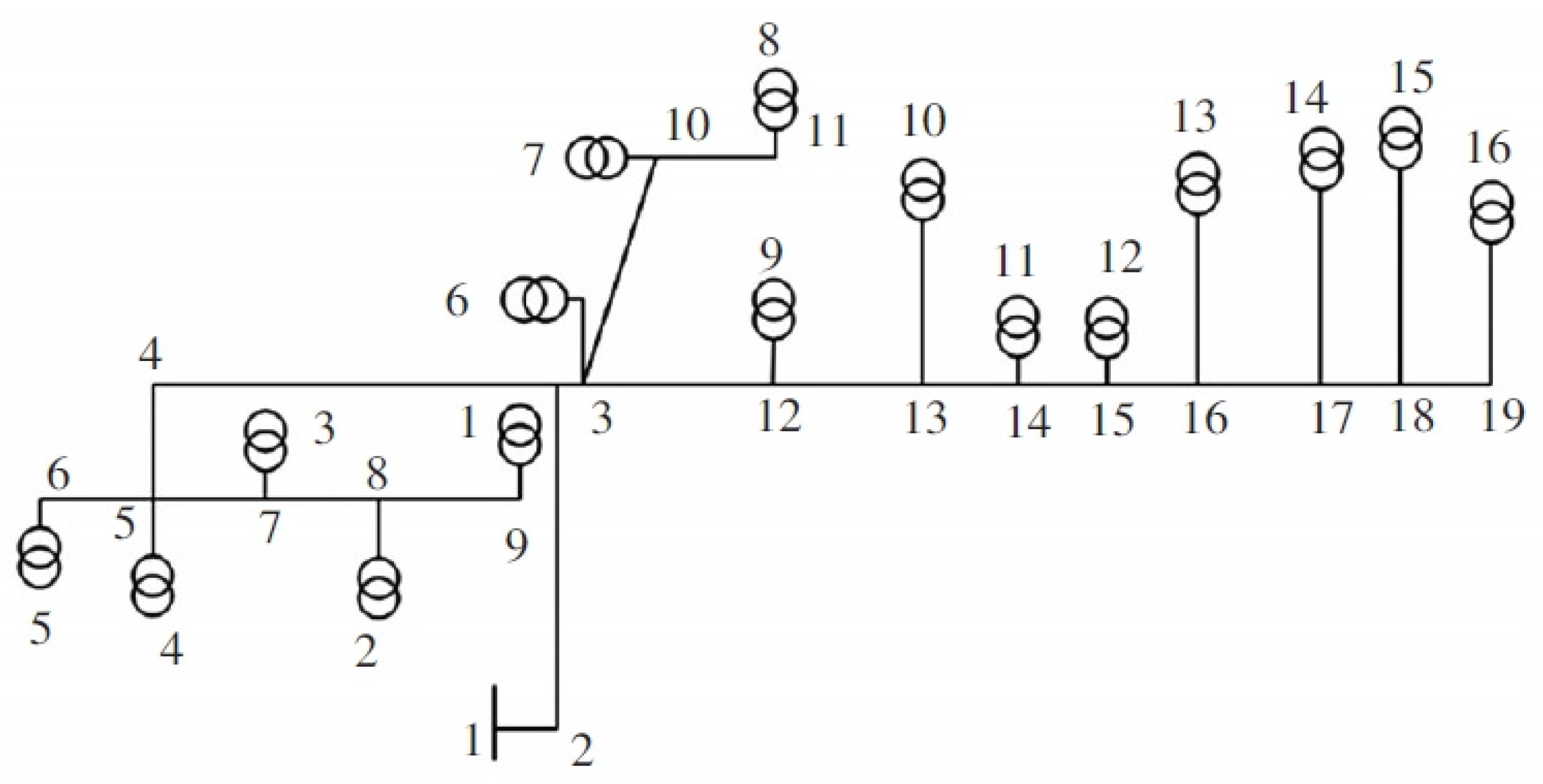
A small region within the provincial power grid was selected as a sample to illustrate the application process and effectiveness of the methods proposed in this paper. In fact, this study conducted experiments at key substations and transmission lines across the entire province, using 10 kV as an illustrative example. The results from other power supply areas were nearly identical and thus not reiterated for brevity. The schematic diagram of the line structure of the simple case is shown in Figure 2.
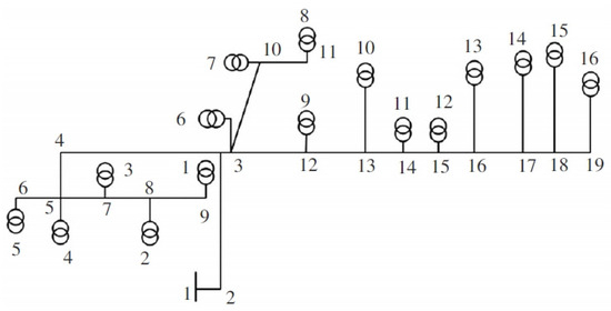
Figure 2.
Schematic of the line structure. The Digits in the figure represent the transformers.
4.2.1. Data
The operational data, which were provided by the grid company, for each distribution transformer are detailed in Table 3, where MMR denotes monthly meter reading, which is the electricity usage record for that line, and AAP, ARP and ALF denote average active power, average reactive power and average load factor, respectively, which are all the attributes of the network.
Table 3.
Operational data for each distribution transformer.
The key parameters related to the cost are set as follows. The cost of each transformer is CNY 15,000 per unit. Generally, the installation and dismantling fees for replacing a distribution transformer are 30% of the purchase price of the equipment. The expenses for line modification are based on the comprehensive investment costs for 10 kV lines. Drawing from a previous study [12] and incorporating findings from actual field surveys, the acquisition cost for reactive power compensation equipment is set at CNY 20 per kvar, with the labor cost also established at CNY 20 per kvar.
4.2.2. Solutions
Replacing conductors, upgrading transformers, and enhancing reactive power compensation are three common methods for reducing grid losses. Specifically, in this case, conductor replacement involves updating Lines 1, 2, and 11. The transformer upgrade involves replacing the eighth transformer with a higher-capacity model (e.g., S11-400), which is due to the fact that the eighth transformer has reached an average load rate of 72.3%. Reactive power compensation involves increasing the power factor of each distribution transformer to 0.9, thereby enabling them to handle a greater load.
The three methods above can be used in any combination, thus resulting in eight strategies, as shown in Table 4, depending on whether or not a particular method is selected. In Table 1, RC, UT, and EC denote replacing conductors, upgrading transformers, and enhancing reactive power compensation, respectively. In the table, the 0–1 variables indicate whether the corresponding strategies have been adopted. PLB and PLA denote the expected power loss before and after the loss reduction strategy is applied.
Table 4.
Operation data of distribution transformers.
Different loss reduction strategies vary in cost and effectiveness. One can employ an enumeration method to calculate the impact of each strategy on the objective function, thereby identifying the optimal strategy that yields the minimum value for the objective function. Alternatively, one could employ the genetic algorithm described in Section 3, treating the selection of loss reduction methods as binary decision variables, and generate the optimal strategy, which includes the decision that minimizes the objective function.
The genetic algorithm illustrated in Figure 1 was implemented through the following steps.
Step 1: Initialization. Initialize the maximum number of evolutionary generations (in this case, ). Randomly generate (in this case, ) individuals using binary encoding to form the initial population , which represents the initial set of loss reduction strategies.
Step 2: Individual judgement. Calculate the fitness value for each individual within the population . Retain the best individual and directly replicate it into the next generation.
Step 3: perform genetic operations, including selection, crossover, and mutation, on the current population , which then generate the next generation .
Step 4: calculate the objective function in the current iteration.
Step 5: Iterate Step 2 to Step 4 until the termination condition is met. The termination conditions include reaching the maximum number of iterations, or the objective function has converged. In this paper, convergence is defined as the difference in the objective function value between two consecutive iterations being within 1%.
The decisions generated in the last iteration formed the optimal strategy. Table 5 shows the optimal strategy, as well as the second one. In the optimal solution, only EC method is applied. The annual investment, direct and indirect loss associated with such strategy are 264.4, 43,080 and 9520.37, respectively, which result in a total cost of 52,864.77. Strategy 3 is suboptimal, as it requires an investment of 1950 and generates direct losses of 41,760 and indirect losses of 9229.
Table 5.
Optimal and suboptimal solutions.
To validate the accuracy of the approach presented in this paper, the objective functions for each strategy were determined using an exhaustive enumeration method, as illustrated in Figure 3.
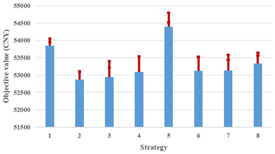
Figure 3.
The results of each loss reduction strategy. The unit on the Y-axis is CNY. The red parts are error bars.
The results clearly demonstrate that the optimal solution is indeed consistent with the outcomes derived from the enhanced genetic algorithm. There is always some deviation in the power grid loss during each measurement, meaning that PLA and PLB have uncertainty. This is the main reason for plotting the error bar in this figure. This is a simple case, as it includes only three loss reduction strategies; thus, exhaustive enumeration requires merely eight possible combinations. When dealing with a large number of possible combinations, the enumeration method may not provide the desired solution within a reasonable time; therefore, the genetic algorithm offers a viable and efficient alternative.
4.2.3. Sensitivity Analysis
The optimal strategy presented in this case study is derived under the parameters specified within this paper. It is acknowledged that changes in energy prices and carbon penalties may alter the optimal strategy. The optimal solution results when these two parameters are, respectively, decreased and increased by 50% are shown in Table 6.
Table 6.
Optimal solutions with different parameters.
Table 6 shows that when these two parameters decrease, the benefits of loss reduction will become increasingly smaller, and the optimal strategy will tend towards the solution with the least investment. Therefore, to promote the adoption of loss reduction strategies in the power grid, increasing the carbon emission penalty is a viable administrative measure.
This paper also conducted a sensitivity analysis on thermal power. The proportion of thermal power was gradually increased from 0.5 to 0.8 in increments of 0.05, and the objective values corresponding to each strategy during this process are presented in Figure 4.
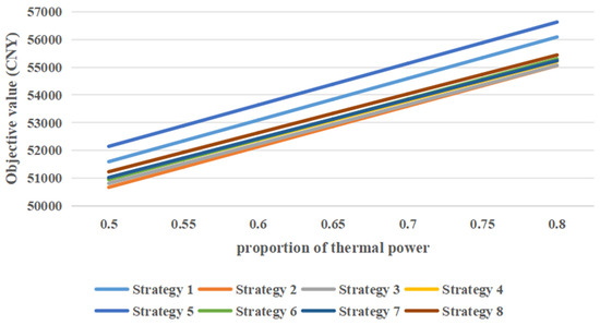
Figure 4.
The results of each loss reduction strategy when the proportion of thermal power varies from 0.5 to 0.8.
It can be seen from Figure 4 that as the proportion of thermal power increases, all objective values show a linear growth trend. The same result also applies to the parameter of the carbon emission factor.
4.3. Application in the Provincial Power Gird Company
This section will take the typical operation mode of the power grid in the province as an example and apply the optimization method proposed in this paper to evaluate the power grid loss and loss reduction results. The company encompasses over 5000 small areas, as illustrated in Section 4.2. Given that each of these small areas has eight different loss reduction strategies, the total number of viable options for the entire company exceeds 800. Consequently, an exhaustive approach becomes entirely impractical at this juncture, necessitating the adoption of the methodology proposed in this paper for decision-making.
4.3.1. Power Grid Loss Distribution
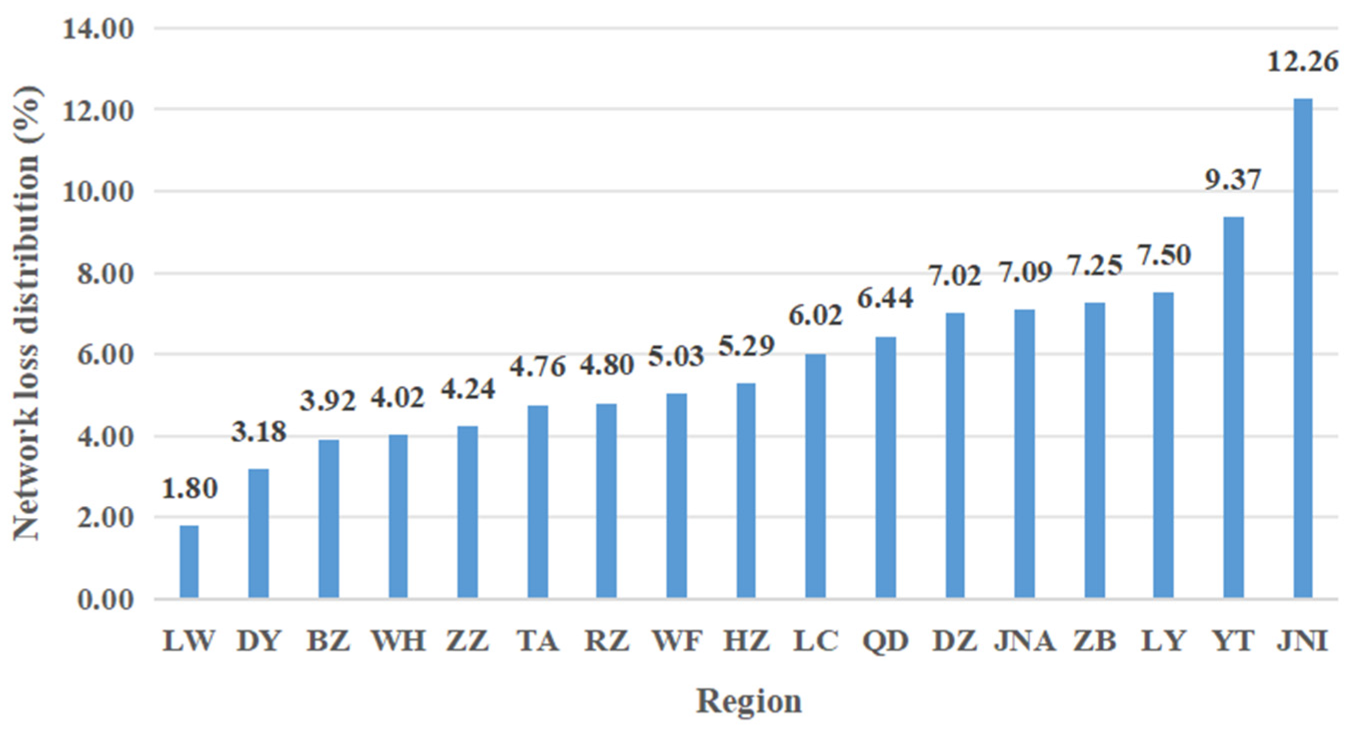
Figure 5 shows the network loss distribution ratio statistics according to different administrative regions. It can be seen that the network loss in JNI, YT, LY, ZB, JNA and DZ is serious, while in regions such as DY, BZ, and WH, the loss is relatively low.
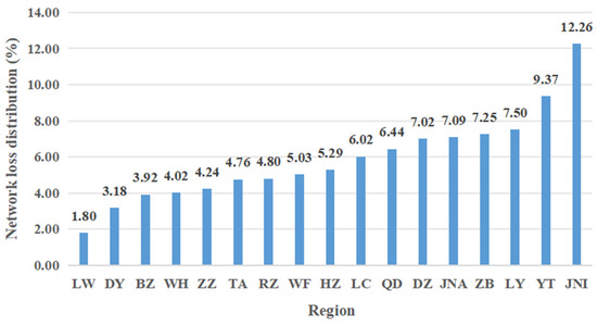
Figure 5.
Network loss distribution ratio in different administrative regions.
4.3.2. Analysis of Loss Reduction Potential
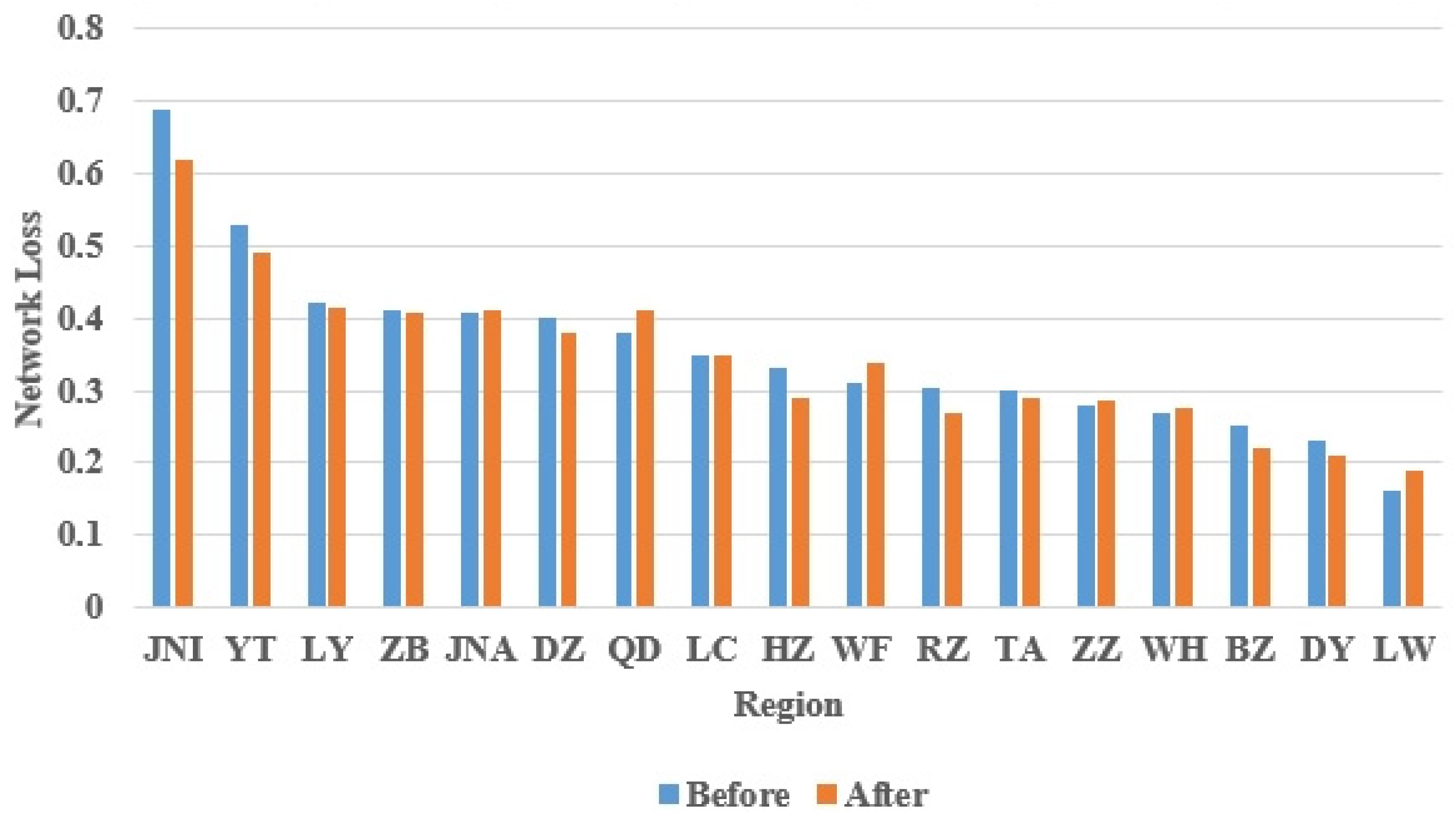
The proposed loss reduction method is applied on the nodes with heavy load and low voltage. After optimization, the loss of the 500 kV and 220 kV transmission grids of the company is reduced from 566.8 MW to 552.9 MW, with a loss reduction of 13.9 MW. Based on the carbon emission intensity of 0.85 t/(MW·h), the reduced carbon emission per unit time is 11.815 t/h. The loss reduction result of power grids in various regions is shown in Figure 6.
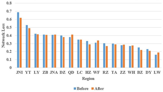
Figure 6.
Comparison of power loss for different regions in the power network.
Among them, the regions with the most obvious loss reduction are JNI and YT. It should be pointed out that the optimization result is to minimize the total network loss of the entire system. Although the network loss in regions such as LW and WF increased after optimization, this is a consideration of sacrificing local interests to maximize global interests.
The application of the proposed model raises practical implementation challenges such as coordination between regions and data granularity. Addressing these barriers is crucial for successful implementation. To mitigate coordination issues, establishing clear communication channels and standardized protocols for data sharing and strategy alignment across regions is essential. For data granularity, implementing robust data collection systems and ensuring data consistency through standardized measurement practices can enhance the model’s accuracy. Additionally, adopting a phased implementation approach allows for gradual integration and adjustment, reducing complexity and enabling continuous optimization.
4.4. Discussion
- (1)
- Potential synergies with renewable energy sources and technologies
In the case study presented in this paper, only three loss reduction methods, i.e., replacing conductors, upgrading transformers, and enhancing reactive power compensation, are considered. With the proliferation of renewable energy sources, the number of approaches to grid loss reduction is also increasing, potentially leading to more efficient loss reduction strategies [11]. However, these changes merely add dimensions to the decision-making process without affecting the applicability of the model proposed here.
- (2)
- Economic concerns
This paper aimed to identify the optimal combination of loss reduction strategies by minimizing the total sum of investment costs, direct costs, and indirect costs. The decrease in direct and indirect costs can be construed as an increase in revenue. Following a previous study [33], we are able to calculate the payback period for various schemes with a risk-free rate of 3%. Take strategy 2 as an example to illustrate the calculation method. With strategy 2, the reduction in power loss is 88,192 − 86,160 = 2032 kW·h. Thus, the direct and indirect cost decrease CNY 1060 and CNY 224.53, respectively. The payback period n refers to the number of years required to recoup the investment of strategy 2, which is CNY 2644, given a revenue of CNY 1240.53 per year. This involves solving the following equation:
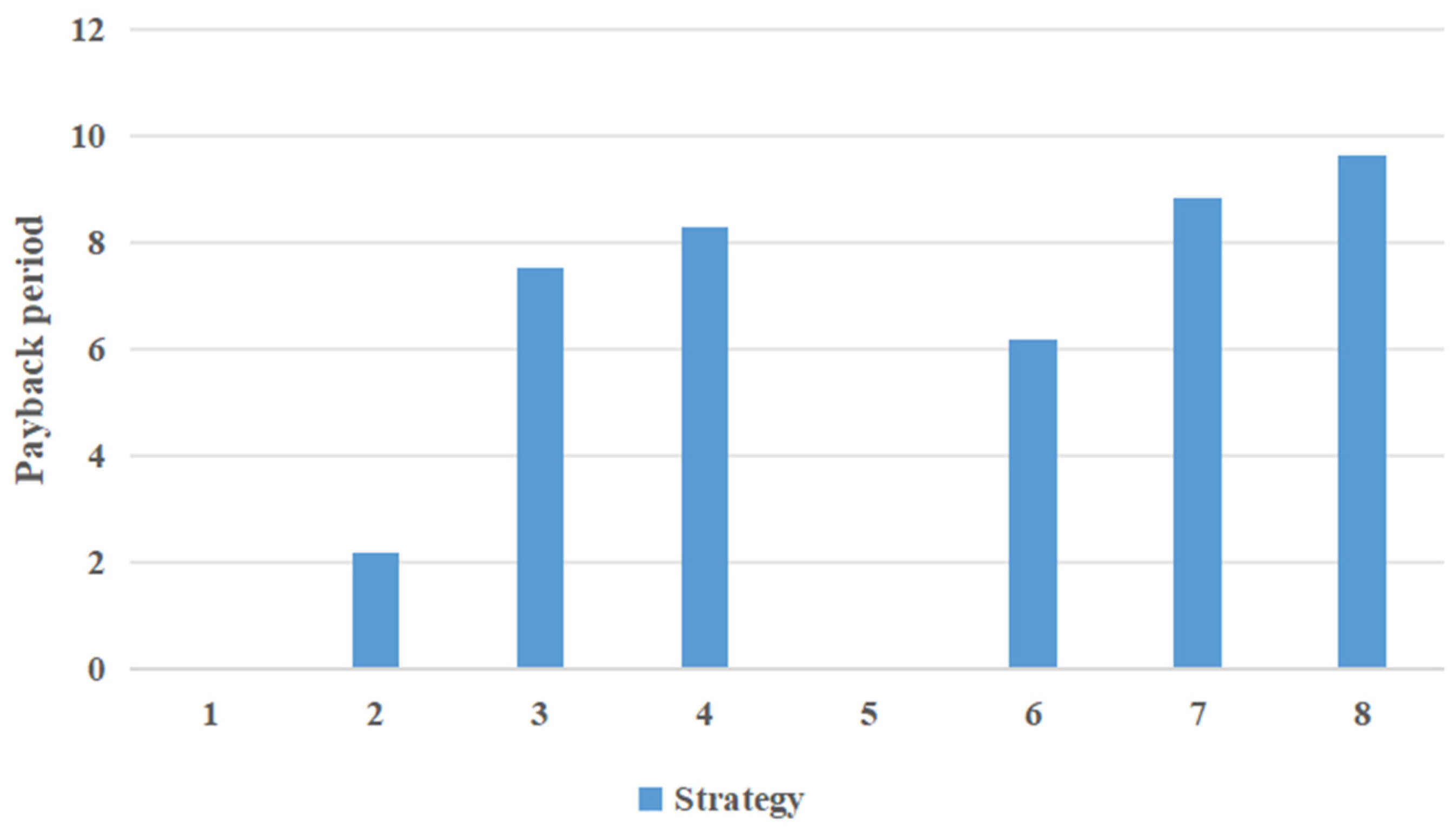
Figure 7 presents the investment payback times for each loss reduction strategy within the small-scale case study detailed in Section 4.2.

Figure 7.
Comparison of payback period for different strategies.
The first strategy where the investment is zero and the fifth strategy where the investment cannot be recovered have no payback period. Among others, the optimal strategy from a cost perspective also has the shortest payback period, a mere 2.17 years. However, the second-best strategy exhibits a considerably longer payback period of 7.51 years, ranking it third in terms of cost efficiency.
In addition to the risk-free rate, inflation and maintenance costs can also impact the payback period. Inflation erodes the purchasing power of money over time, meaning that future cash flows will have less value in today’s terms. If inflation is not accounted for, the payback period may appear shorter than it actually is in real economic terms. Maintenance costs are an ongoing expense that can significantly impact the net cash flows of grid loss reduction strategies. Overlooking these costs may lead to an underestimation of the total investment required. Including maintenance costs in the economic analysis would provide a more accurate picture of the long-term financial commitment associated with each strategy.
- (3)
- Scalability of the model and optimization method
While the current case study focuses on a small sample with three primary loss reduction strategies (replacing conductors, upgrading transformers, and reactive power compensation), the model’s modular design allows for the easy integration of additional loss reduction strategies, ensuring its applicability to broader and more intricate grid configurations. This flexibility is further enhanced by the use of an adaptive genetic algorithm (AGA), which dynamically adjusts its parameters based on the fitness of the population. This feature ensures that the optimization process remains efficient and effective even as the number of strategies and variables increases. The model’s generalization capabilities are supported by its flexibility in handling diverse grid configurations. By adjusting input parameters and constraints, the model can be tailored to specific regional or national grid characteristics. This adaptability is crucial for addressing the unique challenges faced by different power grid systems, such as varying load profiles, voltage levels, and regulatory requirements.
Considering AGA, when the solution space dimension increases, the population size typically needs to be enlarged to maintain diversity and prevent premature convergence, which directly increases the computational effort per generation, including fitness evaluation, crossover, and mutation operations. While the AGA may reduce ineffective searches by dynamically adjusting mutation and crossover rates, thereby maintaining diversity with a smaller population, the complexity of fitness evaluation can still grow nonlinearly with the dimension of the solution space. This is especially true when fitness depends on simulations or experiments, as the time for a single evaluation cannot be reduced through algorithmic optimization. In this study, the number of optional strategy combinations is limited. Even considering technological development, combining some methods in advance can effectively reduce the solution space. Thus, the algorithm’s scalability is not a major concern.
- (4)
- Effect of the trend
In the current model, the objective function is formulated based on a static assumption of electricity prices and carbon penalties over the lifecycle of the strategies. This approach simplifies the optimization process and allows for a clear evaluation of the cost–benefit trade-offs associated with different grid loss reduction measures. However, it does not capture the potential variability in these parameters, which can be influenced by market conditions, regulatory changes, and technological advancements. For instance, a gradual increase in carbon penalties (e.g., due to stricter climate policies) could incentivize higher upfront investments in loss reduction measures. Conversely, a decrease or elimination of carbon penalties would diminish the importance of carbon-related costs in the optimization process.
To demonstrate it, the following numerical experiment is conducted in this paper. It is assumed that the carbon penalty increases linearly over time, as is shown in Equation (20).
Using this formula, the price of the carbon penalty for each future year is calculated and then substituted into the optimization model, yielding the following results (shown in Figure 8).
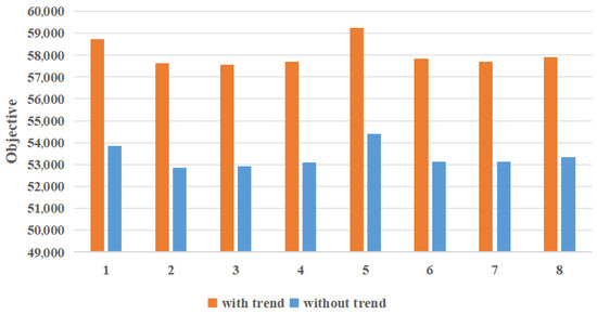
Figure 8.
Results of each loss reduction strategy with and without linear carbon penalty trend.
It can be seen that the objective value of all strategies has increased, while the optimal strategy remains unchanged. Then, this formula is also incorporated into the payback period calculation, and Figure 9 illustrates that the payback period for all strategies has increased.
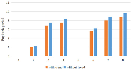
Figure 9.
Results of payback period with and without linear carbon penalty trend.
This is consistent with the previous analysis. The same result also applies to the parameter of electricity prices.
5. Conclusions
In the context of electricity price reforms, power grid companies are urgently in need of tapping into potential loss reduction and optimizing loss mitigation measures to reduce grid losses through technical means. This necessity becomes even more critical in the backdrop of a low-carbon agenda. This paper proposes an optimization method for selecting loss reduction strategies in distribution networks that considers the benefits of low-carbon initiatives. It provides a theoretical foundation for the optimization of loss reduction strategies in distribution networks, addressing the challenge of quantitatively selecting loss reduction strategies. The model was validated through illustrative examples, demonstrating its good applicability and operability. We have also applied this method to the optimization of loss reduction in provincial power grids, and the results demonstrate that the method possesses excellent adaptability.
This paper contributes to proposing an optimization model for selecting loss reduction strategies in distribution networks, considering the low-carbon benefits. The model is designed to minimize the total cost, which includes the comprehensive investment in loss reduction measures (such as equipment purchase, removal, installation, or reconstruction), direct loss costs due to energy loss, and indirect loss costs. Voltage deviation and branch power serve as constraints in the model. Additionally, depending on the actual situation, the model can optionally include constraints on the number of loss reduction measures and total investment. This flexibility makes the model more adaptable to various scenarios.
While this study has demonstrated the potential of the proposed optimization model, several avenues for future research remain open. One promising direction is the integration of renewable energy sources into the grid loss reduction strategies. As renewable energy becomes more prevalent, the dynamic nature of these energy sources introduces new challenges and opportunities for grid management. Future work could explore how the proposed model can be adapted to incorporate renewable energy integration, thereby enhancing the grid’s resilience and sustainability.
Another area for further investigation is the development of more advanced optimization algorithms to improve computational efficiency. As the complexity of power grids increases, the need for faster and more accurate optimization methods becomes critical. Research into hybrid algorithms or machine learning techniques could potentially enhance the model’s performance and scalability.
Author Contributions
Conceptualization, W.L., Q.X., X.W., Z.L., T.L. and D.Z.; methodology, W.L., Q.X., X.W., Z.L., T.L. and D.Z.; software, W.L., Q.X., X.W., Z.L., T.L. and D.Z.; writing—original draft preparation, W.L., Q.X., X.W., Z.L., T.L. and D.Z. All authors have read and agreed to the published version of the manuscript.
Funding
This research was funded by the Technical Service Project of State Grid Jiangsu Electric Power Co., Ltd. (Grant No.: W24FZ2730030).
Data Availability Statement
The data are available from the corresponding author on reasonable request.
Conflicts of Interest
Authors Weiwu Li, Qing Xu, Xinying Wang, Zhengying Liu and Tianshou Li were employed by the State Grid Gansu Electric Power Co., Ltd. The remaining authors declare that the research was conducted in the absence of any commercial or financial relationships that could be construed as a potential conflict of interest.
References
- Pang, B.; Zhang, L.H.; Ten, Y.F.; Chang, Z.W.; Tang, C.; Hu, C.Q.; Liu, Z.W.; Wang, B.L. An incentive scheme of peak-valley price based on differential privacy. J. Chongqing Univ. 2023, 46, 56–68. [Google Scholar]
- Yu, X.; Dong, Z.; Zheng, D.; Deng, S. Analysis of critical peak electricity price optimization model considering coal consumption rate of power generation side. Environ. Sci. Pollut. Res. 2024, 31, 41514–41528. [Google Scholar] [CrossRef]
- Tian, X.; Niu, X.; Zhu, X.; Zhao, G. Optimal strategy and assessment method for minimizing power loss of Shandong power network under lowcarbon background. Autom. Electr. Power Syst. 2014, 38, 67–72. [Google Scholar]
- Bouakkaz, A.; Gil Mena, A.J.; Haddad, S.; Ferrari, M.L. Efficient energy scheduling considering cost reduction and energy saving in hybrid energy system with energy storage. J. Energy Storage 2021, 33, 101887. [Google Scholar] [CrossRef]
- Eid, A. Cost-based analysis and optimization of distributed generations and shunt capacitors incorporated into distribution systems with nonlinear demand modeling. Expert Syst. Appl. 2022, 198, 116844. [Google Scholar] [CrossRef]
- Li, C.; Xu, D. Family of enhanced ZCS single-stage single-phase isolated AC–DC converter for high-power high-voltage DC supply. IEEE Trans. Ind. Electron. 2017, 64, 3629–3639. [Google Scholar] [CrossRef]
- Long, Y.; Wang, X.Y.; Zhou, Q.; An, H.Y.; Chen, Z. Distribution network reconfiguration for loss reduction considering maximum power supply capability index. Proc. CSU-EPSA 2017, 29, 131–134. [Google Scholar]
- Sadeghian, O.; Moradzadeh, A.; Mohammadi-Ivatloo, B.; Abapour, M.; Anvari-Moghaddam, A.; Lim, J.S.; Marquez, F.P.G. A comprehensive review on energy saving options and saving potential in low voltage electricity distribution networks: Building and public lighting. Sustain. Cities Soc. 2021, 72, 103064. [Google Scholar] [CrossRef]
- Sambaiah, K.S.; Jayabarathi, T. Loss minimization techniques for optimal operation and planning of distribution systems: A review of different methodologies. Int. Trans. Electr. Energy Syst. 2020, 30, e12230. [Google Scholar] [CrossRef]
- Sun, K.; Xiao, H.; Liu, S.; You, S.; Yang, F.; Dong, Y.; Wang, W.; Liu, Y. A Review of Clean Electricity Policies—From Countries to Utilities. Sustainability 2020, 12, 7946. [Google Scholar] [CrossRef]
- Kyriakopoulos, G.L. Energy Communities Overview: Managerial Policies, Economic Aspects, Technologies, and Models. J. Risk Financ. Manag. 2022, 15, 521. [Google Scholar] [CrossRef]
- Lazzeroni, P.; Repetto, M. Optimal planning of battery systems for power losses reduction in distribution grids. Electr. Power Syst. Res. 2019, 167, 94–112. [Google Scholar] [CrossRef]
- Xie, J.; Chen, C.; Long, H. A loss reduction optimization method for distribution network based on combined power loss reduction strategy. Complexity 2021, 2021, 9475754. [Google Scholar] [CrossRef]
- Wang, W.; Cai, D.; Liu, H.; Zhou, C.; Cao, K.; Zhou, K.; Liu, C. Theoretical Analysis of Power Loss Reduction for Typical Power Grid. In Proceedings of the ICASIT 2020: 2020 International Conference on Aviation Safety and Information Technology, Weihai, China, 14–16 October 2020; pp. 383–387. [Google Scholar]
- Suresh, M.; Edward, J.B. A hybrid algorithm based optimal placement of DG units for loss reduction in the distribution system. Appl. Soft Comput. 2020, 91, 106191. [Google Scholar] [CrossRef]
- Pokhrel, B.R.; Karthikeyan, N.; Bak-Jensen, B.; Pillai, J.R. Loss optimization in distribution networks with distributed generation. In Proceedings of the 2017 52nd International Universities Power Engineering Conference (UPEC 2017), Heraklion, Greece, 28–31 August 2017; pp. 1–6. [Google Scholar]
- Ahmadi, I.; Ahmadigorji, M.; Tohidifar, E. A novel approach for power loss reduction in distribution networks considering budget constraint. Int. Trans. Electr. Energy Syst. 2018, 28, e2635. [Google Scholar] [CrossRef]
- Iweh, C.D.; Gyamfi, S.; Tanyi, E.; Effah-Donyina, E. Distributed Generation and Renewable Energy Integration into the Grid: Prerequisites, Push Factors, Practical Options, Issues and Merits. Energies 2021, 14, 5375. [Google Scholar] [CrossRef]
- Kataray, T.; Nitesh, B.; Yarram, B.; Sinha, S.; Cuce, E.; Shaik, S.; Vigneshwaran, P.; Roy, A. Integration of smart grid with renewable energy sources: Opportunities and challenges–A comprehensive review. Sustain. Energy Technol. Assess. 2023, 58, 103363. [Google Scholar] [CrossRef]
- Alotaibi, I.; Abido, M.A.; Khalid, M.; Savkin, A.V. A comprehensive review of recent advances in smart grids: A sustainable future with renewable energy resources. Energies 2020, 13, 6269. [Google Scholar] [CrossRef]
- Mu, H.; Pei, Z.; Wang, H.; Li, N.; Duan, Y. Optimal Strategy for Low-Carbon Development of Power Industry in Northeast China Considering the ‘Dual Carbon’ Goal. Energies 2022, 15, 6455. [Google Scholar] [CrossRef]
- Zhang, Y.; Wang, X.; Wang, J.; Zhang, Y. Deep Reinforcement Learning Based Volt-VAR Optimization in Smart Distribution Systems. IEEE Trans. Smart Grid 2020, 12, 361–371. [Google Scholar] [CrossRef]
- Zhang, L.; Zhang, K.; Zhang, G. Power distribution system reconfiguration based on genetic algorithm. In Proceedings of the 2016 IEEE Advanced Information Management, Communicates, Electronic and Automation Control Conference (IMCEC), Xi’an, China, 3–5 October 2016; pp. 80–84. [Google Scholar]
- Sehgal, S.; Swarnkar, A.; Gupta, N.; Niazi, K.R. Reconfiguration of distribution network for loss reduction at different load schemes. In Proceedings of the 2012 IEEE Students’ Conference on Electrical, Electronics and Computer Science (SCEECS), Bhopal, India, 1–2 March 2012; pp. 1–4. [Google Scholar]
- Gautam, M.; Bhusal, N.; Benidris, M.; Louis, S. A Spanning Tree-based Genetic Algorithm for Distribution Network Reconfiguration. In Proceedings of the 2020 IEEE Industry Applications Society Annual Meeting, Detroit, MI, USA, 10–16 October 2020; pp. 1–6. [Google Scholar]
- Kamel, S.; Hamour, H.; Nasrat, L.; Yu, J.; Xie, K.; Khasanov, M. Radial distribution system reconfiguration for real power losses reduction by using salp swarm optimization algorithm. In Proceedings of the 2019 IEEE Innovative Smart Grid Technologies—Asia (ISGT Asia), Chengdu, China, 21–24 May 2019; pp. 720–725. [Google Scholar]
- Wu, H.; Li, T.; Chen, H.; Li, B.; Liu, T. Distribution network line loss optimization method based on war strategy algorithm. In Proceedings of the 2023 8th Asia Conference on Power and Electrical Engineering (ACPEE), Tianjin, China, 14–16 April 2023; pp. 395–402. [Google Scholar]
- Zhang, L.; Yan, Y.; Xu, W.; Sun, J.; Zhang, Y. Carbon emission calculation and influencing factor analysis based on industrial big data in the “double carbon” era. Comput. Intell. Neurosci. 2022, 2022, 2815940. [Google Scholar] [CrossRef] [PubMed]
- Wan, Y.; Hou, H.; Ge, X.D.; Wang, X.H.; Lu, Y.C.; Wang, Y.X. Two-stage mixed-game win-win strategy for integrated energy system considering multi-stage utilization of carbon emission. Autom. Electr. Power Syst. 2025, 49, 69–79. [Google Scholar]
- Zheng, W.; Wu, W.; Zhang, B.; Sun, H.; Liu, Y. A fully distributed reactive power optimization and control method for active distribution networks. IEEE Trans. Smart Grid 2015, 7, 1021–1033. [Google Scholar] [CrossRef]
- Srinivas, M.; Patnaik, L. Adaptive probabilities of crossover and mutation in genetic algorithms. IEEE Trans. Syst. Man. Cybern. 1994, 24, 656–667. [Google Scholar] [CrossRef]
- Zhai, L.; Feng, S. A novel evacuation path planning method based on improved genetic algorithm. J. Intell. Fuzzy Syst. 2022, 42, 1813–1823. [Google Scholar] [CrossRef]
- Eberhart, R.; Kennedy, J. A new optimizer using particle swarm theory. In Proceedings of the Sixth International Symposium on Micro Machine and Human Science, Nagoya, Japan, 4–6 October 1995; pp. 39–43. [Google Scholar]
- Zhan, Z.H.; Zhang, J.; Li, Y.; Chung, H.S.H. Adaptive Particle Swarm Optimization. IEEE Trans. Syst. Man Cybern. Part B Cybern. 2009, 39, 1362–1381. [Google Scholar] [CrossRef]


Disclaimer/Publisher’s Note: The statements, opinions and data contained in all publications are solely those of the individual author(s) and contributor(s) and not of MDPI and/or the editor(s). MDPI and/or the editor(s) disclaim responsibility for any injury to people or property resulting from any ideas, methods, instructions or products referred to in the content. |
© 2025 by the authors. Licensee MDPI, Basel, Switzerland. This article is an open access article distributed under the terms and conditions of the Creative Commons Attribution (CC BY) license (https://creativecommons.org/licenses/by/4.0/).