Abstract
Carbon capture, utilization, and storage (CCUS) is an emerging technology with significant potential for large-scale emissions reduction. To reduce the overall system costs of CCUS, this study first establishes a comprehensive economic cost model for the entire CCUS process. Subsequently, a Monte Carlo-based Sobol’ global sensitivity analysis method is proposed to calculate both first-order and total-order sensitivity indices, followed by qualitative and quantitative analyses of parameter sensitivity. Additionally, convergence analyses of the results and their engineering applicability are examined. The findings reveal that the total-order sensitivity indices for electricity price, flue gas inlet flow rate, pipeline diameter, pipeline material price, pipeline inlet pressure, and injection pressure are 0.6578, 0.3857, 0.5585, 0.3823, 0.2205, and 0.1949, respectively, which are significantly higher than those of the other parameters. This indicates that these parameters have a dominant impact on energy consumption costs through the processes of capture and compression, pipeline transportation, and storage injection. These results provide a basis for selecting decision variables when optimizing the entire CCUS process.
1. Introduction
With the continuous emission of greenhouse gases, global climate change, which is mainly caused by greenhouse gases emitted by human activities such as fossil fuel burning and land-use changes, has gradually become a major threat to human sustainable development [1]. The CO2 content in all of the gases emitted accounts for more than two-thirds of the total amount of greenhouse gases, and this is one of the main factors in global climate warming. CO2 capture, utilization, and storage (CCUS), as an emerging technology with large-scale emissions reduction potential, is expected to achieve near-zero CO2 emissions from fossil energy use [2], and it is considered to be one of the most important technical solutions for reducing greenhouse gas emissions [3].
Although CCUS technology has great potential, its high economic cost has become one of the main obstacles hindering its development. A large number of studies have been designed and optimized for CCUS systems in order to reduce the system cost. Rao et al. [4] discussed the research status of various CO2 capture technologies and the design details of CO2 capture systems, providing a comprehensive evaluation of the techno-economic, environmental, and other aspects. Zhang et al. [5] developed an economic model based on the hydrodynamic model of CO2 pipeline transport and carried out economic optimization and evaluation of the CO2 pipeline transportation system. Dong-Hun Kwak et al. [6] introduced a CO2 supply plan, established a CO2-EOR dynamic model and an economic–environmental optimization model, and optimized the model through genetic algorithms to maximize the net present value. Nasim Elahia et al. [7] focused on the overall system optimization of the UK’s commercial CO2 supply, transportation, and storage chain, establishing a multi-period minimum cost optimization model and solving it using mixed-integer linear programming methods, making optimal investment and operational decisions. Zimmermann et al. [8] developed a detailed guideline for systematic techno-economic analysis (TEA) and life-cycle assessment (LCA) for CCUS technologies, aiming at improving the comparability of TEA studies, leading to improved decision-making and more efficient allocation of funds and time resources for the research, development, and deployment of CCUS technologies. Maselli et al. [9] developed and validated an innovative and integrated methodology called Life-Cycle Cost and Sustainability Assessment (LCC-SA), which allows for the joint assessment of project life-cycle costs and socio-cultural and environmental externalities. However, it can be found that there are some characteristics (such as complex models, high dimensions, and large amounts of calculation) that can lead to the inaccuracy of the optimization results.
In order to solve this problem, it is necessary to use the sensitivity analysis method to select the important parameter factors and determine the priority of parameters in the CCUS whole-process system model [10,11]. It is well known that sensitivity analysis plays a significant role in modeling, calibration, verification, scenario analysis, uncertainty analysis, and decision-making. Sensitivity analysis usually includes local sensitivity analysis (LSA) and global sensitivity analysis (GSA). LSA considers changes in one parameter at a time, while keeping the other parameters unchanged. Many researchers have made significant contributions, advancing the application of the LSA method in engineering applications for CCUS parameter sensitivity analysis. Koelbl et al. [12] established a technical economic model based on the CO2 capture and storage process, and they conducted sensitivity analysis of the uncertainty of technical and economic parameters. Belaissaoui et al. [13] performed a steady-state sensitivity analysis of the CO2 capture process and correlated it with process operability and control to find the optimal design, operating conditions, and control strategies. Shang et al. [14] considered the influence of different reservoirs and fluid properties on oil well productivity, and they conducted a sensitivity analysis on the factors affecting the production capacity of CO2 flooding wells. However, LSA only considers the change in a single parameter and does not account for the interactions between parameters.
To address the limitations of LSA, GSA has been enhanced to analyze the combined effects of multiple parameters and their interactions across the entire parameter space, making it more suitable for complex system analysis. Common global sensitivity analysis methods in CCUS include the Morris screening method, FAST method, and Sobol’ method. The Morris method is a screening-based approach that calculates the Elementary Effect (EE) for each input variable and evaluates the variables’ importance through statistical analysis. Ali et al. [15] selected 27 thermodynamic and structural design variables as input parameters for sensitivity analysis, and they evaluated the effects of three actual crude oil compositions on the gas–oil ratio (GOR) and CO2 content changes based on the Morris screening method. The research of Giovanni and Georgios et al. [16,17] also shows that this method has great potential in the fields of LCA and energy system optimization. While it provides qualitative metrics, it cannot quantify the specific impact of factors on the output, making it ideal for initial screening when the number of input variables is large and rapid identification of important variables is needed. The FAST method, based on Fourier-transform techniques, maps input variables to a frequency domain and assesses the variables’ importance through the frequency response of the model’s outputs. The study by Satola and Dela et al. [18,19] found that the FAST method and the Sobol’ method use similar sensitivity indicators to calculate parameters’ significance, and both can detect the complex interactions between variables, but the FAST method considers only nonlinear effects and neglects interactions between variables. Due to their computational efficiency and simplicity, both the FAST and Morris methods are widely used when computational resources are limited or rapid evaluation of sensitive variables is required. The Sobol’ method, based on variance decomposition, allocates the total variance of the model outputs to individual variables and their interactions, clarifying each variable’s contribution to the output variation. This method is particularly effective for nonlinear and complex models. Comparative studies by Kucherenko and Tang et al. [20,21] have shown that the Sobol’ method is efficient, offering better sensitivity rankings and being well suited for evaluating multi-parameter interactions. Jiri Nossent and Homma et al. [22,23] demonstrated its successful application to complex environmental and nonlinear models. In addition, many scholars have incorporated machine learning, mixed sensitivity analysis techniques, and other methods into sensitivity analysis. For example, Vreman et al. [24] discussed advances of classic DSA methods and their implications, exploring the technical specifications, options for presenting results, and implications for decision-making associated with each method. Jakeman et al. [25] presented an adaptive algorithm based on multi-index stochastic collocation, which can be used for uncertainty quantification (UQ) and sensitivity analysis (SA) at a fraction of the cost of a purely high-fidelity approach. Yan et al. [26] addressed the main steps of the CCUS value chain and explored how ML is playing a leading role in expanding the knowledge across all fields of CCUS. Shang et al. [27] proposed an efficient method based on a multi-fidelity kriging (cokriging) surrogate model; tests demonstrated that the cokriging estimator is an efficient approach to yield promising accuracy and reduce computational costs in the sensitivity analysis.
However, the variance decomposition approach requires numerous model evaluations, making it challenging to apply accurately to high-dimensional models with many parameters. In this case, Gaussian Process Regression (GPR) and Bayesian methods may be more advantageous, especially in cases with limited sample sizes. Bayesian [28] inference combines priors and observation data to update the posterior distribution of parameters, providing comprehensive quantification of parameter uncertainty and allowing for inference in complex models. GPR [29] is a non-parametric Bayesian method that is used to estimate the response surface of complex systems. It can provide predictive means and uncertainty measures, suitable for sensitivity analysis in small-sample situations. However, these two methods require more computing resources and complex model settings, which may significantly increase the cost of exemplary CCUS projects. Taking the GPR method as an example, its computational complexity increases exponentially with the data size as the number of samples increases [30]. Due to these limitations, standard GPR models become impractical for large datasets.
Therefore, this paper proposes a Monte Carlo sensitivity analysis method for the CCUS system, based on the Sobol’ method and Monte Carlo estimation, for the sensitivity analysis of model parameters in the entire CCUS process. This method uses the economic cost of the entire CCUS process as the objective function and selects a range of interacting engineering and economic parameters, including flue gas inlet flow (), flue gas inlet temperature (), solution concentration (), pipe diameter (), pipe inlet pressure (), pipe material price (), injection well inlet pressure (), injection well inlet flow () and injection depth (), and electricity price (), as candidate factors. The first-order and total-order sensitivity indices of key parameters in the CCUS system are calculated, followed by convergence analysis and sensitivity ranking. The results provide a more precise method for selecting decision variables during the CCUS whole-process optimization, thereby improving the optimization efficiency and enhancing the accuracy of the optimization results.
The remainder of this paper is structured as follows: Section 2 provides a brief introduction to the Sobol’ method, the principles of the Monte Carlo-based Sobol’ method, and the framework for sensitivity analysis of the carbon capture, utilization, and storage (CCUS) whole-process system. Section 3 focuses on the modeling of the CCUS whole-process system and the design of the global sensitivity analysis (GSA) algorithm, detailing the model construction of the CCUS subsystems, the establishment of a whole-process economic cost model, the GSA algorithm for the CCUS whole-process system, and the characteristics and selection of the parameters within these models. Section 4 discusses the results of the sensitivity analysis, including convergence and applicability. Finally, Section 5 concludes this paper.
2. Research Methodology
2.1. Sobol’ GSA Method
The Sobol’ method, introduced in 1993 [31], is a global sensitivity analysis approach based on variance. It decomposes the model into functions of individual input variables and combinations of multiple input variables. These functions consist of 2N terms derived from multiple integrals. By quantifying the contribution of each variable (or variable combination) to the total output variance, the corresponding sensitivity coefficients are calculated.
It is supposed that a general mathematical model function is defined as , and it is a square-integrable function; is an indeterminate model input , in which is a selected univariate model output. Furthermore, it is assumed that the model inputs are independent and uniformly distributed within the unit hypercube . This assumption is no loss of generality, because any input space can be converted to this unit hypercube [32]. The Sobol’ method is based on the decomposition of variance, as follows [33,34]:
where is a constant, denotes the function of , denotes the function of and , and so on.
A condition of this decomposition is satisfied as follows:
Sobol’ proved the uniqueness and mutual orthogonality of the above decomposition, which can be obtained through multiple integrals, as shown below:
Using the above method, all terms can be obtained. Since the model function is square-integrable, the total variance of f(X) is as follows:
The variance of each term can be obtained by calculating each corresponding component of (X):
Since the terms fi, fij, and f1,2,…,k are mutually orthogonal, squaring both sides of Equation (1) and rearranging the terms will yield the decomposition of the variance expression, as follows:
The sensitivity coefficients of each order are defined as the ratio of the partial variance of each order to the total variance. The s-order sensitivity Si1, Si2, …, Sis is defined as follows:
2.2. Monte Carlo-Based Sobol’ GSA Method
Because the CCUS system model is complex and nonlinear, it is almost impossible to calculate the variances by using analytical integrals. Hence, the Monte Carlo estimation is used to calculate the integral to reduce the calculation error.
As can be seen from Equation (2), all terms in the functional decomposition are orthogonal, which leads to the definition of the terms in the functional decomposition in terms of conditional expected values:
Therefore, Formula (8) can be expressed as follows:
where the X~i notation indicates the set of all variables except Xi. The above variance decomposition shows how the variance of the model output can be decomposed into terms attributable to each input, as well as the interaction effects between them. Together, all terms sum to the total variance of the model output.
The first-order sensitivity index and main effect index are respectively defined as follows [35,36]:
where denotes first-order indices, which measure the main effect of output variance varying alone; denotes the total effect index, which measures all variances caused by the interaction with any other input variables; is the expected reduction in variance that would be obtained if could be fixed; and and are the expected variance and the expected reduction in variance that would be obtained if all factors but could be fixed, respectively [37]. One can divide the other terms in the variance decomposition by to obtain the higher-order interaction indices , , etc. Both and are nonnegative and satisfy the formula . In general, the mathematical model is a function with multidimensional integrals (as in Equation (2)), which requires other mathematical calculation methods to compute the variances.
The Monte Carlo estimator is a kind of calculation algorithm based on random sampling to obtain numerical results. Its basic idea is to use randomness to solve problems that may be deterministic in principle. This study assumes that the number of design parameters of the system is , randomly samples times in the initial space of all design parameters, and simultaneously extracts two sample matrices of the form and , where each row of the matrices represents a combination of parameters [38].
According to the above sample matrix, and can be defined, in which the -th column of matrix (or ) and the -th column of matrix (or ) can be exchanged, and the remaining parameters remain unchanged.
In order to calculate the sensitivity indices and , the expectation operators and variance first need to be calculated. According to the above sample matrix hypothesis, and can be calculated by using the Monte Carlo estimator, as follows [39]:
2.3. GSA Framework for the Whole-Process CCUS System
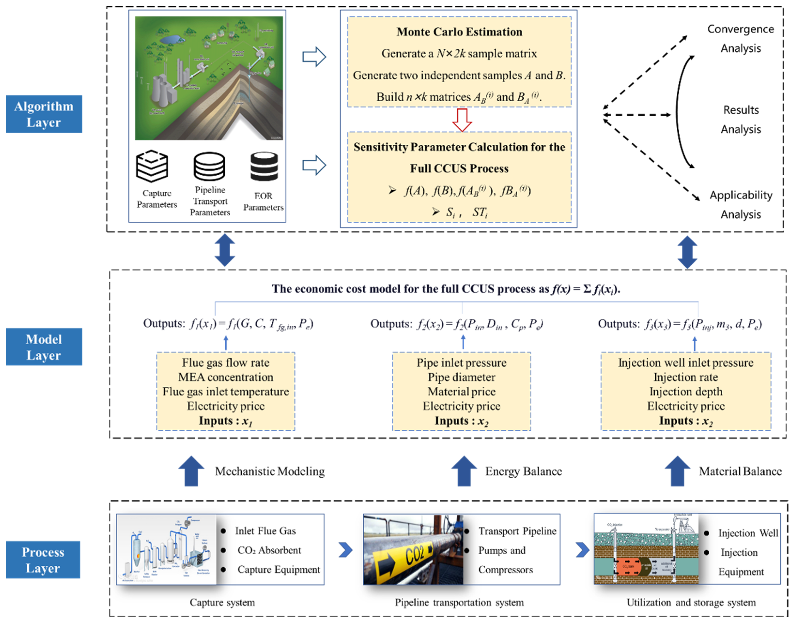
Given the complexity of the entire CCUS process, this study develops a multidimensional, multi-hierarchical global sensitivity analysis framework for the full-chain CCUS system, employing the Sobol’ method with Monte Carlo estimation. The framework quantifies the impact of key parameter variations on the system’s economics. It employs an integrated “parameter, model, algorithm” approach and features a modular architecture with three core levels: process, model, and algorithm, as shown in Figure 1.

Figure 1.
GSA framework for the whole-process CCUS system.
The process level focuses on key input parameters, including flue gas flow rate, MEA concentration, and electricity price. Using mechanistic modeling based on energy and material balances, it maps core parameters to process operations in capture, transportation, and storage systems, forming the data foundation for further analysis. The model level develops a total cost model, expressed as f(X) = ∑f(Xi), where f1, f2, and f3 correspond to the cost functions of capture, transportation, and storage, respectively. It integrates technical parameters and cost data, forming the modeling basis for sensitivity analysis. The algorithm level applies the Sobol’ GSA method using Monte Carlo estimation. It generates an N × 2k sample matrix for random sampling and statistical analysis, quantifying the impact of parameter variations on system costs. Additionally, convergence and applicability analyses assess the reliability and relevance of sensitivity results in optimizing CCUS system costs in engineering practice.
3. CCUS Whole-Process System Modeling and Design of GSA Algorithms
3.1. Overview of CCUS Processes
CCUS, the abbreviation for carbon capture, utilization, and storage, is one of the key technologies to address global climate change. It includes four components: capture, transportation, utilization and storage [40].
- (1)
- Carbon capture module
The chemical absorption method is widely used in the carbon capture stage; therefore, this paper adopts a post-combustion capture system based on an MEA solution in coal-fired power plants [41]. The operational process is as follows: flue gas generated by coal-fired power plants enters the absorption tower, where CO2 undergoes reversible chemical reactions with the MEA solution for absorption, while non-CO2 gases are discharged. The CO2-rich MEA solution then enters the regeneration tower, where high-purity CO2 is released through heating, and the regenerated MEA solution is recycled back to the absorption tower for reuse. With a designed capture efficiency of 90%, the module not only ensures significant carbon reduction but also balances regeneration energy consumption and costs. As the core carbon source acquisition component of the CCUS system, this module provides a stable gas supply for subsequent transportation and storage, with its performance directly influencing the carbon capture scale and the economic efficiency of the entire process [42].
- (2)
- Pipeline transportation module
The pipeline transportation module plays a crucial role in efficiently and safely transferring captured CO2 from capture facilities to storage or utilization sites [43]. This paper uses a terrestrial high-pressure liquid CO2 pipeline system with a design pressure of 10.3–15.3 MPa and a transportation distance of 200 km. This pressure range keeps the CO2 in a supercritical state, combining the gaseous diffusivity with the liquid-like high density to reduce the transportation energy consumption. The pipeline is made of high-strength carbon steel, with its diameter optimized based on flow rate and pressure drop calculations to balance initial investment and operational costs. During transportation, pumping stations are installed to compensate for pressure loss, with the station spacing determined by pipeline frictional resistance, CO2 physical properties (density, viscosity), and terrain. Multi-stage compression is used to maintain stable pressure. As the “carbon transportation bridge” of the CCUS system, this module enables long-distance, large-scale carbon transfer via high-pressure liquid transportation, providing a stable supply for the storage module and serving as the critical hub connecting the capture and storage components [5].
- (3)
- Utilization and storage module
The utilization and storage module is a key component in achieving closed-loop carbon reduction through CCUS, enabling efficient carbon conversion and permanent isolation by integrating resource utilization with geological storage [44]. In the utilization segment, CO2 generates economic value primarily through enhanced oil recovery (EOR), chemical feedstock production, and applications in food and medicine. Currently, the most widely adopted method is using CO2 for enhanced oil recovery, which boosts crude oil recovery by 15–20%. As such, this study focuses specifically on the technical approach of using CO2 for oil reservoir displacement and storage. The enhanced oil recovery (EOR) and storage segment utilizes geological technologies to inject CO2 into depleted oil and gas reservoirs for displacement and long-term storage. CO2 injection into these reservoirs enhances crude oil recovery by boosting production by 15–20%. This method effectively uses CO2 to displace residual oil, while simultaneously ensuring its permanent storage. The storage process relies on geological formations to securely trap the CO2 and prevent its release into the atmosphere. Although this approach offers significant economic benefits through increased oil recovery, it faces challenges such as limited monitoring technologies and restrictions on the scale of utilization. Future efforts should focus on improving CO2 injection techniques, developing more efficient monitoring systems, and enhancing the overall scalability of CO2 storage and utilization, ultimately advancing CCUS towards a circular carbon economy [45].
3.2. Economic Cost Model
3.2.1. Capture Module
The economic cost model of the capture system is mainly composed of four parts: capture equipment investment, compressor and pump investment, operation and maintenance costs, and electricity costs. Among these, electricity costs account for the largest proportion in the economic cost model of the capture system. The following are the specific economic cost models for each part:
- (1)
- Investment in trapping equipment
Using the 0.6 power method to model each device [46], the total investment cost of the equipment is as follows:
where and are the capacity and cost index of the equipment, respectively, while denotes the type of equipment (cooler, blower, absorption tower, heat exchanger, reboiler, regeneration tower, condenser, MEA recycler, pump and compressor, etc.).
where is the investment cost of the cooler (CNY 10,000), is the flue gas blower investment cost (CNY 10,000), is the absorption tower investment cost (CNY 10,000), is the heat exchanger investment cost (CNY 10,000), is the regeneration tower investment cost (CNY 10,000), is the investment cost for the reboiler (CNY 10,000), is the investment cost for the solution reboiler (CNY 10,000), and is the investment cost for the other equipment (CNY 10,000).
- (2)
- Investment in compressors and pumps
According to the literature [47,48], the maximum power of the compressor unit under the current technical conditions is . The number of compressor units required should be an integer, and then the number of parallel compressor units should be .
Compressor investment (CNY 10,000):
Pump investment (CNY 10,000):
where is the reference compressor cost (CNY 10,000), is the capacity of the compressor (kw), and is the capacity of the pump (kw).
- (3)
- Operation and maintenance costs
Operation and maintenance costs mainly include fixed costs (equipment materials, labor, etc.) and variable costs (chemical consumption, fuel, water treatment, etc.).
where , , and are the price of the MEA solution, water (), and steam per unit mass (), respectively; and are the quality of MEA and water consumed per one ton of CO2 captured (kg/tCO2), respectively; represents other costs; and represents the system operating time (years).
- (4)
- Electricity cost estimate
The electricity bill mainly comes from the energy consumption of the compressor/pump and the steam demand, so the electricity bill is estimated as follows [49]:
where is the thermoelectric conversion coefficient, is the electricity price (), is the system operating time (h), and is the electricity cost of the CO2 capture system (CNY 10,000).
In summary, the economic cost model is as follows:
The relevant parameters of the economic cost model for the capture process are shown in Table 1.

Table 1.
The relevant parameters of the economic cost model for the capture process.
3.2.2. Pipeline Transportation Module
The economic cost model of the pipeline transportation system is mainly composed of four parts: pipeline construction investment, pump station investment, operation and maintenance costs, and electricity costs. Among these, pipeline construction investment accounts for the largest proportion in the economic cost model of the pipeline transportation system. The following are the specific economic cost models for each part:
- (1)
- Investment in pipeline construction
Pipeline transportation system investment costs [50,51]:
where is the cost of the pipe materials (), is the total mass of steel for the pipeline (kg), is the pipe wall thickness (m), is the inner diameter of the pipeline (m), is the pipe length (km), and is the material cost factor.
- (2)
- Pump station investment
Pump station investment can be calculated based on the following formula [52]:
where is the total investment in the pump stations for the pipeline transportation system (CNY 10,000), is the capacity of each pumping station (kw), and is the number of pumping stations.
- (3)
- Operation and maintenance costs
According to some studies of CO2 pipeline transportation, operation and maintenance costs account for a part of the total investment cost [53], calculated by
where is the operation and maintenance cost (CNY 10,000), and is the operation and maintenance coefficient.
- (4)
- Electricity cost estimate
Due to the friction of the pipeline, the pressure will be reduced along the pipeline. In order to meet the transmission requirements, a pumping station needs to be set up to provide power. The electricity bill is mainly determined by the electricity price in the transmission process, the number of pumping stations, the consumption of electric energy, and the system operating time.
The electricity cost is estimated as follows [49]:
where is the electricity price (), is the electric energy consumed by the system (kw), is the number of pumping stations, and is the system operating time (h).
In summary, the economic cost model is as follows:
The relevant parameters of the economic cost model for pipeline transportation are shown in Table 2.
Table 2.
The relevant parameters of the economic cost model for pipeline transportation.
3.2.3. Utilization and Storage Module
The economic cost model of the utilization and storage system is mainly composed of three parts: oil recovery and storage equipment investment, operation and maintenance costs, and electricity costs. Among these, electricity costs account for the largest proportion in the economic cost model of the utilization and storage system. The following are the specific economic cost models for each part:
- (1)
- Utilization and storage equipment investment
The number of injection wells in the utilization and storage module depends on the CO2 flow rate and the injection volume per well. The number of injection wells required is as follows [37,54]:
where is the capital cost of injection well drilling (CNY 10,000/year); is the capital cost of the injection equipment (CNY 10,000/year); is the capital cost for on-site screening and evaluation (CNY 10,000/year); and are the model coefficients of injection well drilling and injection equipment, respectively; and is the total capital cost of the injection well (CNY 10,000/year).
- (2)
- Operation and maintenance costs
Operation and maintenance costs mainly include aboveground and underground maintenance costs, along with other daily costs [37]
where is the cost of surface maintenance (CNY 10,000/year); is the cost of underground maintenance (CNY 10,000/year); is the overhead and consumables cost (CNY 10,000/year); , , and are the model coefficients of surface maintenance, underground maintenance, and overhead and consumption, respectively; and is the operation and maintenance cost for the utilization and storage system (CNY 10,000/year).
Therefore, the total cost of the utilization and storage system in the CCUS whole-process system can be calculated as follows:
- (3)
- Electricity cost estimate
The main sources of power consumption are the processes of carbon dioxide compression, crude oil absorption, and hydrocarbon separation. The total power consumption of the utilization and storage process can be calculated as follows [49]:
Then, the electricity cost can be estimated as follows:
where is the electric energy required for CO2 compression (), is the power consumed by crude oil absorption (), is the electricity consumed by the hydrocarbon separation process (), is the power consumed for other processes of the system (), is the system running time (h), and is the crude oil production (bbl).
Therefore, the CCUS whole-process system electricity charges are as follows:
In summary, the economic cost model is as follows:
The parameters related to the economic cost model of the utilization and storage process are shown in Table 3.
Table 3.
The parameters related to the economic cost model of the utilization and storage process.
3.2.4. Whole-Process Cost Calculation
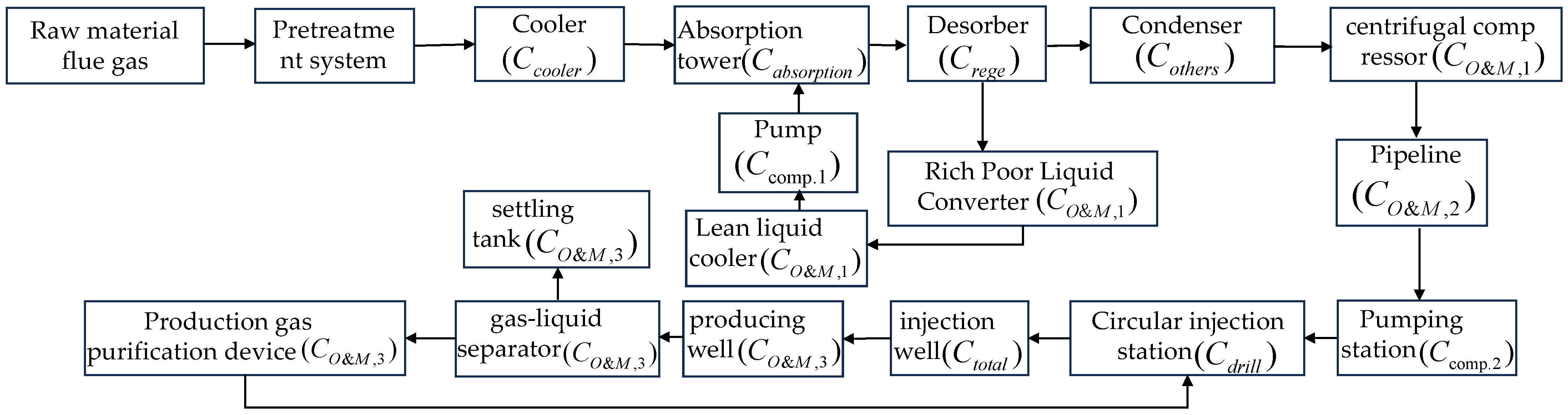
The CCUS whole-process economic cost modeling is the core model for quantifying the economics of carbon capture, pipeline transportation, utilization, and storage systems. By integrating the parameters and economic factors of each stage, it reveals the cost structure of each stage and its key elements, as shown in Figure 2. The model is based on a modular structure and covers the three subsystems of capture, pipeline transportation, and utilization and storage. The total cost model of the whole process of CCUS is as follows:
where ; is the discount rate (%); represents the capital recovery coefficient () of the capture, pipeline transportation, and utilization and storage processes, respectively; and is the corresponding design life (years) of the capture, pipeline transportation, and utilization and storage subsystems.
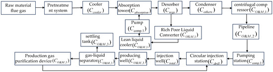
Figure 2.
CCUS whole-process system.
3.3. Variable Description of the Economic Cost Model
Selecting appropriate parameters is a crucial step in the modeling process. Based on CCUS system models constructed in the previous literature [55,56,57,58,59], the main parameters included the flue gas inlet temperature, flue gas inlet flow rate, electricity price, pipeline diameter, pipeline inlet pressure, pipeline operating temperature, pipeline price, injection well inlet pressure, injection well inlet flow rate, and other variables. According to the parameter probability distribution and parameter range, nine key parameters were selected in this study: flue gas inlet flow (), flue gas inlet temperature (), solution concentration (), electricity price (), pipe diameter (), pipe inlet pressure (),pipe material price (), injection well inlet pressure (), injection well inlet flow (), and injection depth (). Table 4 shows the distribution status and range of each parameter.
Table 4.
Parameters studied for the sensitivity analysis.
The parameters selected above demonstrate significant independence in the process design, which is determined by the modular nature of the CCUS system. The technical parameters of each stage are independently optimized according to local process requirements. For instance, in the capture stage, the flue gas inlet flow rate and temperature are primarily determined by the design load of the capture unit, without direct correlation to parameters such as pipeline diameter and pressure in the transportation stage. In the transportation stage, parameters like pipeline material cost and pipeline inlet pressure are determined by independent factors such as transportation distance and geological conditions, without affecting the parameter design of the injection wells. In the storage stage, parameters such as injection depth and injection flow rate are independently determined by the geological storage conditions, without relation to economic parameters like electricity prices.
This paper selects a uniform distribution as the probability distribution of the input variables, which not only aligns with the engineering reality but also meets the initial requirements of sensitivity analysis. The specific reasons are as follows: During the initial stages of CCUS projects, sufficient historical data to support complex distributions (such as normal distribution, Gamma distribution) are lacking. The uniform distribution assumes that parameters appear with equal probability within a given range, covering all possible values and avoiding omissions caused by deviations from the distribution assumption. Secondly, this paper only conducts a preliminary exploration of CCUS cost sensitivity analysis. The goal of preliminary sensitivity analysis is to identify key parameters rather than to make precise predictions. The uniform distribution, by covering the entire parameter range, ensures that the sensitivity of key parameters is fully captured.
3.4. Design of GSA Algorithms for the CCUS Whole-Process System
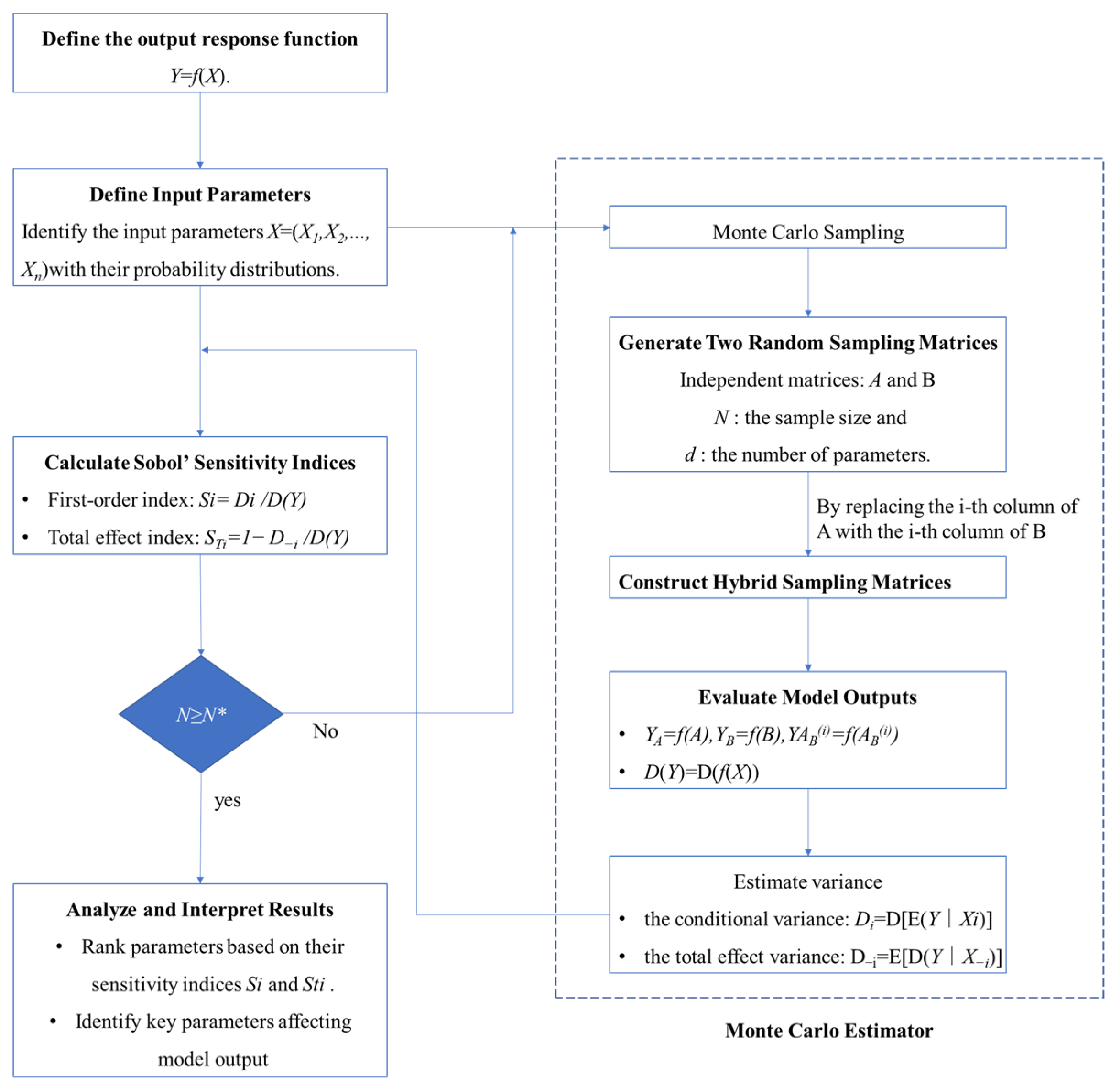
This study employs the Monte Carlo method and Sobol’ sensitivity analysis to quantify the effects of input parameters on the model output. Figure 3 shows the flowchart of the CCUS system sensitivity analysis algorithm. The process defines the response function, parameters, and distributions, followed by Monte Carlo sampling and mixed matrix construction for output evaluation. Variance calculations estimate the parameter contributions, and Sobol’ indices assess the main effects and interactions. Finally, the sample adequacy is verified, sensitivity indices are analyzed, and key parameters are ranked, providing insights for model optimization and uncertainty analysis. The detailed steps of the algorithm are as follows:
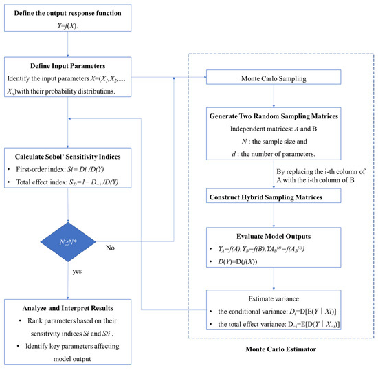
Figure 3.
Flowchart of the GSA algorithm for the CCUS whole-process system.
Step 1: Definition of Analysis Framework. The output response function Y = (X) and input parameters X = (X1, X2, …, Xd) are defined, along with their probability distributions.
Step 2: Monte Carlo Sampling and Sample Generation. Monte Carlo sampling generates two independent random sampling matrices, A and B, with a sample size of N and d parameters. A mixed sampling matrix is constructed by swapping columns between A and B to evaluate the model outputs under different parameter combinations.
Step 3: Model Output Evaluation. The model outputs YA = (A), YB = f(B), and YABi = f(ABi) are computed, along with the variance D(Y). Conditional variance Di = [E(Y∣Xi)] and total effect variance DTi = E[D(Y∣X−i)] are estimated to quantify each input parameter’s contribution to the output variance.
Step 4: Computation of Sobol’ Sensitivity Indices. Sobol’ sensitivity indices, including the first-order index Si = Di/(Y) and the total effect index STi = 1 − D−i/D(Y), are calculated. The first-order index quantifies the main effects of individual input parameters, while the total effect index accounts for both main effects and parameter interactions.
Step 5: Sample Size Verification. The sample size N is compared with the required threshold N*. If N is insufficient, additional sampling is performed before reevaluating the model. If N meets the threshold, the process proceeds to the next step.
Step 6: Sensitivity Index Analysis and Interpretation. The sensitivity indices Si and STi are analyzed, and the input parameters are ranked based on their influence on the model output to identify key parameters.
4. Discussion
4.1. First- and Total-Order Sensitivity Indices
This section describes two sensitivity indices and their 95% confidence intervals (CIs) and parameter sensitivity rankings. As shown in Table 5, the left part of the table shows the first-order sensitivity calculation results, 95% confidence intervals, and ranking numbers (columns 3–5), while the right half represents the total-order sensitivity calculation results, 95% confidence intervals, and ranking numbers (columns 6–8). By comparing the ranking numbers of the parameters (columns 5 and 8), one can clearly see that the parameters , and have higher sensitivity, which directly affects the output of the system model, while the sensitivity of parameters such as , , , and is relatively low, and these have a weak effect on the model output. According to the 95% confidence intervals, only these six parameters have significant sensitivity. It is worth noting that is more effective, so according to the total-order sensitivity index, it is can be seen that the parameter levels are slightly different.
Table 5.
First- and total-order sensitivity indices, confidence intervals, and parameter rankings under different input parameters.
Among the top six parameters, is 0.6578, ranking the highest among all parameters and demonstrating its dominant influence on energy consumption costs. From a technological perspective, every link in CCUS incurs expenses due to electricity utilization, and electricity costs constitute the largest proportion of the total cost parameters (equipment investment costs, electricity bills, and operation and maintenance expenses). Therefore, the sensitivity analysis results align with actual production scenarios. Additionally, , , , , and are 0.5585, 0.3857, 0.3823, 0.2205, and 0.1949, respectively, ranking from second to sixth. Among these factors, directly affects the structural design of the entire pipeline transportation system, thereby influencing the overall investment in transportation processes. will determine the scale of the entire CCUS system and is a key parameter of the system. The pipe inlet pressure , pipe diameter , and pipe material price are the main parameters determining the cost of pipeline transportation, so these parameters have strong sensitivity to the model output. Finally, the injection well inlet pressure is the key parameter for determining the cost of the injection equipment and injection pipeline, ranking fifth among all of the system parameters.
Among the top six parameters, the width of the confidence intervals of is 0.8788, which is about 5.5 times the width of , which is only 0.1596. This result indicates that the value of for the sample is very stable for , while it fluctuates greatly for . In order to visually and clearly identify the outliers in the data, this paper uses a boxplot, as shown in Figure 4. The median of the sample data is located at the center of the boxplot (red line), the length of the box represents the interquartile range, and the ends of the box must be the upper and lower limits. Outliers are defined as sample data points that are greater than or less than . The boxplot can not only reflect the characteristics of a dataset’s distribution but also determine whether the distribution of normal values is concentrated or scattered. The upper box pattern (Figure 4a–c) represents the first-order sensitivity , and the lower box pattern (Figure 4d–f) represents . The difference between and represents the interaction of this parameter with all other parameters. For example, the difference in is about 0.2352, indicating that it has a strong interaction with the other parameters. At the same time, the size of the rectangular box indicates the degree of dispersion of the data. The rectangular box of the parameter has a large area, indicating that the data are relatively scattered. , , , , , and are less dispersed. Furthermore, , , and are not well shown due to their low sensitivity.
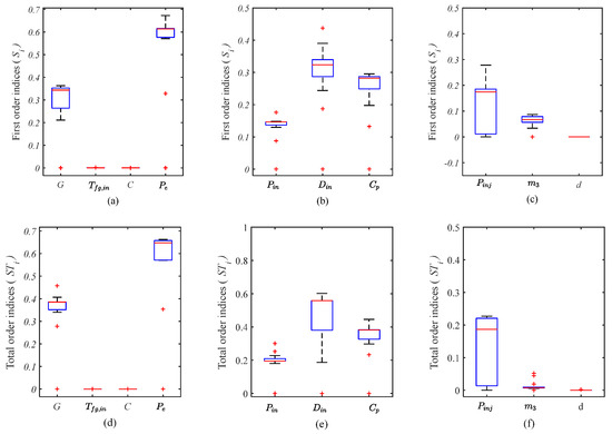
Figure 4.
First- and total-order indices of different parameters in the CCUS system. (a) first-order sensitivity indices for the variables , , , and ; (b) first-order sensitivity indices for the variables , , and ; (c) first-order sensitivity indices for the variables , and ; (d) total-order sensitivity indices for the variables , , , and ; (e) total-order sensitivity indices for the variables , , and ; (f) total-order sensitivity indices for the variables , and .
4.2. Convergence Analysis of Sensitivity Results
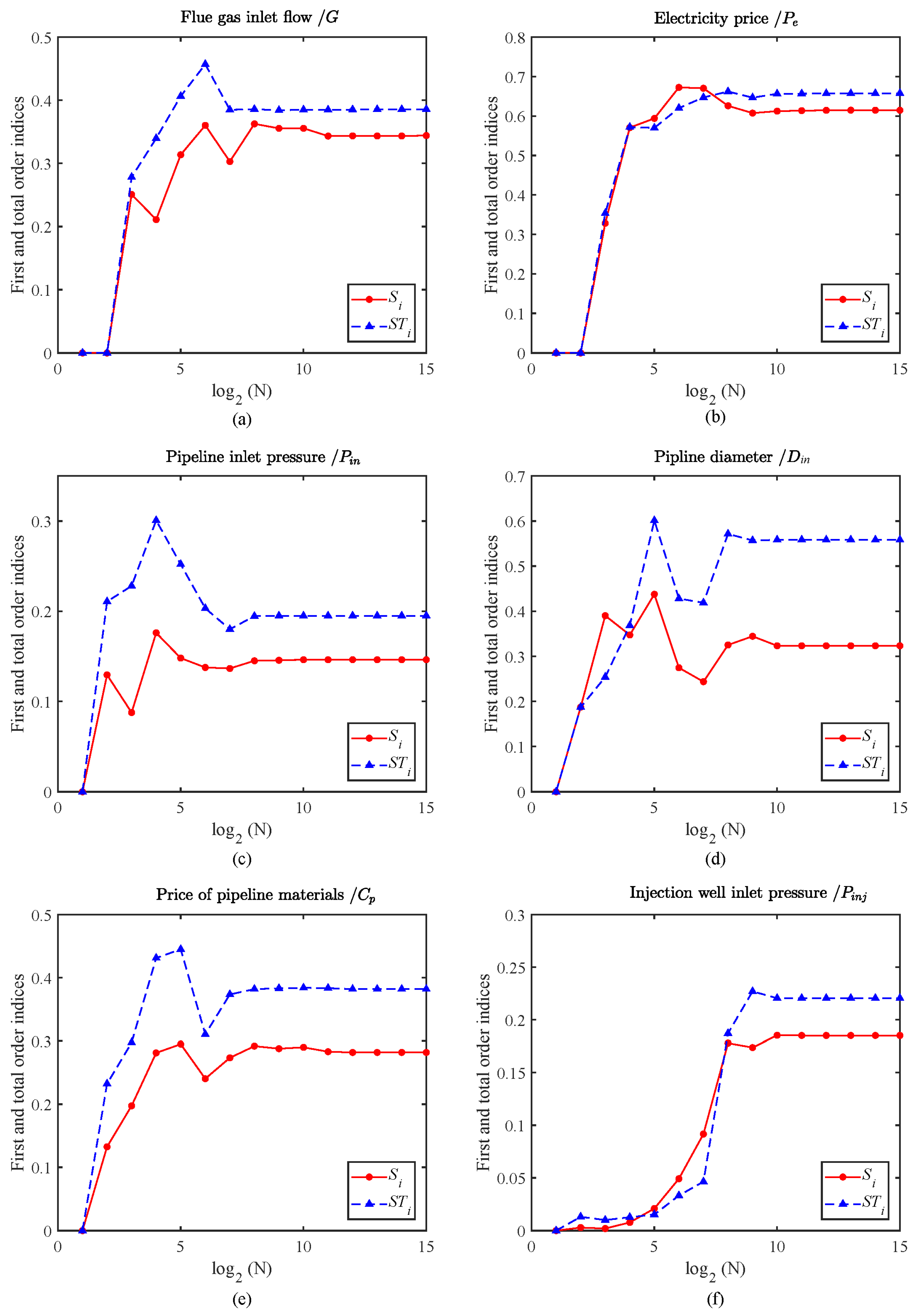
The concept of convergence refers to the process in which, as the sample size or number of calculations increases, the analysis results gradually stabilize and approach the true value. In sensitivity analysis, if the basic sample size is N and the number of parameters is p, then at least N model runs are required to calculate the corresponding sensitivity indices, which often implies a significant sample size requirement. To ensure the reliability and validity of the results in this study, it was crucial to analyze the stability and convergence rate of the sensitivity analysis results. Therefore, a further analysis of the convergence of the results was carried out. Kucherenko et al. [22] suggests that, when random sampling sequences are used, the best convergence performance is achieved when the sample size is a power of two. Based on this, this study explores and calculates the convergence of the sensitivity indices for G, Pe, Pin, Din, Cp, and Pin with a sample size of 2N, and the evolution of the sensitivity indices at different sampling stages is shown in Figure 5.
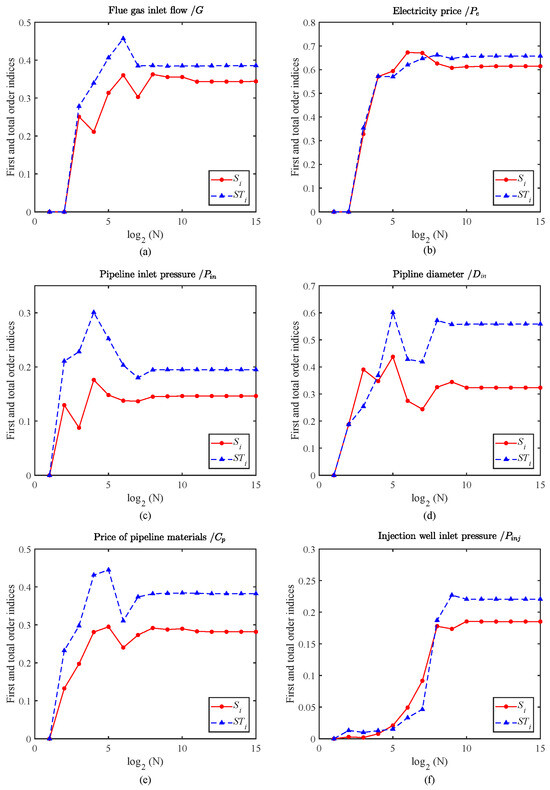
Figure 5.
Evolution of the first- and total-order sensitivity of key parameters with higher sensitivity index. (a) Evolution of the sensitivity indices for the flue gas inlet flow, ; (b) Evolution of the sensitivity indices for the electricity price, ; (c) Evolution of the sensitivity indices for the pipeline inlet pressure, ; (d) Evolution of the sensitivity indices for the pipeline diameter, ; (e) Evolution of the sensitivity indices for Price of pipeline materials, ; (f) Evolution of the sensitivity indices for the injection well inlet pressure, .
Figure 5 shows the relationship between the sensitivity index and the basic sample size , which is helpful to visually judge the convergence of the sensitivity index and the evolution of the simulation results. According to the analysis of the first- and total-order sensitivity in Section 4.1, it can be seen that , and have higher sensitivity in the CCUS system, so only the convergence and evolution of these six parameters are analyzed here. In general, it should be noted that the total-order sensitivity index () is higher than the first-order sensitivity index (). Figure 5a shows the evolution of the first-order and total-order sensitivity indices of the flue gas inlet flow , where it can be seen that when the sample size is small, the first-order and total-order sensitivity indices fluctuate greatly and cannot converge. When the sample size () is gradually increased, the curve value tends to be flat, and when is equal to 8192 (), it can achieve convergence. At the same time, the greater the difference between the two curves, the more obvious the interaction among the parameters. In addition, the evolution of the other parameters’ (, , , , and ) sensitivity indices (Figure 5b–f) is similar to that of , and they have the same convergence characteristics.
The Monte Carlo integration method estimates an integral I as , where I represents the estimated integral, N is the sample size, and (xi) denotes the function values at sampled points xi. The Monte Carlo estimator is defined as . Since the samples (xi) are independent and identically distributed, the expectation of IN is , which shows that IN is an unbiased estimator of the true integral I. The variance in IN is given by . Using the properties of variance, . Since all samples are independent and identically distributed, we denote , so . This implies that the estimation error follows a normal distribution with a mean of 0 and variance of σ2/N, which means that . According to the variance calculation formula, we can obtain . Therefore, the error of the Monte Carlo method can be defined as . From the CLT result, the error is proportional to the standard deviation: . As the standard deviation of the estimation error is proportional to , with the increase in sample size N in powers of two, the estimation errors of both the first-order sensitivity index and the total-order sensitivity index STi show a downward trend. When the sample size is small, the convergence rate of the sensitivity index values is relatively fast, but the estimated values fluctuate greatly, which may be caused by the randomness of the Monte Carlo method. As the sample size increases, the convergence rate gradually slows down. Ultimately, the Monte Carlo estimates converge to the true values, and the error distribution can be approximated by a normal distribution. The experimental results provide empirical support for the applicability of Monte Carlo estimation in sensitivity analysis, indicating that the theory has guiding significance in practical applications. Furthermore, the convergence analysis of the Monte Carlo method was validated in a CCUS project at a Chinese oilfield, showing strong agreement with the operational data, thereby confirming its effectiveness in parameter optimization for practical engineering.
4.3. Applicability Analysis of Sensitivity Analysis Results
From a practical project perspective, sensitivity analysis can provide guidance for engineering and policy decisions, and its applicability has been proven in some articles. For example, Shirmohammadi R et al. [60] used changes in the main parameters for sensitivity calculation, to evaluate the main parameters such as capture efficiency, the heat consumption removed, and the working capacity of the plant. Rawat A et al. [61] analyzed the main parameters affecting the CO2 injection effect by applying various sensitivity methods, such as proxy models, Morris analysis, and the Sobol’ method. The analysis then produced an optimization framework highlighting conditions conducive to achieving maximum oil recovery. The above articles discuss how sensitivity analysis results can guide and optimize actual production processes. Therefore, this section will discuss how to use sensitivity analysis results to optimize operational strategies and apply them to economic feasibility studies and policymaking.
Existing research has extensively modeled and optimized CCUS systems to reduce system costs. Current studies indicate that CCUS systems are complex, multi-input systems characterized by high model complexity, numerous parameters, and strong nonlinearities. During optimization processes, improper selection of decision parameters may lead to low optimization efficiency and inaccurate results. Sensitivity analysis methods aim to address these challenges by identifying critical input parameters, prioritizing their significance, reducing the model parameters’ dimensionality, refining model structures, and selecting highly sensitive parameters to inform CCUS system modeling and optimization decisions. Specific applications include (1) determining parameters requiring further investigation to reduce output uncertainty, (2) identifying irrelevant parameters for elimination from the final model, (3) assessing inputs with the greatest contribution to output variability, and (4) evaluating parameters demonstrating the highest correlation with system outputs.
Additionally, sensitivity analysis of key parameters can also be utilized in economic feasibility studies and policy formulation guidance. Governments can design differentiated subsidies based on the results of sensitivity analysis, offering higher subsidy rates to technological R&D with high sensitivity parameters to expedite technological breakthroughs. For example, as analyzed in this article, the pipeline inlet pressure, pipe diameter, and pipe material prices exhibit strong sensitivities to the model outputs; therefore, cost balance points can be identified through optimizing the transportation network design. In terms of policy guidance, real-time monitoring of high-sensitivity parameters should be implemented. Based on sensitivity analysis, parameter safety thresholds and technical standards can be established. For instance, sensitivity analysis indicates that exceeding critical pressure values leads to exponential growth in energy consumption, necessitating the setting of pressure caps. Furthermore, governments can incorporate sensitivity analysis results into project approval processes by formulating policies. New projects are required to submit parameter sensitivity reports to demonstrate their controllability with respect to economic and safety aspects. Norway’s Sleipner Project serves as a typical case [62]. Through sensitivity analysis, it was discovered that the injection well pressure had the most significant impact on storage efficiency. After optimization, the storage rate increased by 12%, while costs decreased by 9%.
5. Conclusions
This study preliminarily applied sensitivity analysis methods to investigate the parameter sensitivity of the CCUS economic model. Initially, the first-order and total-order sensitivity indices of 10 critical parameters in the CCUS system model were calculated by integrating the Sobol’ method with Monte Carlo estimation techniques. Subsequently, convergence analysis was conducted on both first-order and total-order sensitivity metrics, with prioritized focus on their ranking sequences. Furthermore, the implications of the sensitivity analysis results for system optimization, policy formulation, and investment decision-making were discussed. The findings indicate that parameters such as pipeline inlet pressure, flue gas inlet flow rate, pipeline diameter, pipeline price, and injection well pressure exhibit relatively large total-order sensitivity indices, suggesting that these parameters have significant impacts on the CCUS system’s objective function and should be prioritized in future CCUS system optimization efforts. In a word, it can be concluded that the obtained results have two important roles: (a) The use of sensitivity analysis methods is conducive to the factor determination and priority selection of the input parameters of the CCUS system model, and they could even be reasonably applied to model evaluation and correction. (b) The research results of this paper provide better guidance and reference to solve the problem of inaccurate parameter selection during CCUS whole-process modeling and optimization. If the more sensitive parameters are considered as decision variables, the optimization efficiency and accuracy will be improved.
This paper only preliminarily explores the application of sensitivity analysis methods in CCUS technology. In future work, it will be necessary to improve and innovate such methods to make them perfectly applicable to various CCUS projects. Therefore, the following prospects are proposed: (1) A mixed sensitivity analysis technique that combines deterministic and stochastic methods: Future hybrid methods may achieve an adaptive balance between computational efficiency and accuracy by dynamically adjusting the weights of deterministic analysis and random sampling. (2) Introducing new optimization algorithms to improve optimization efficiency: In order to improve convergence, optimization measures such as variance reduction techniques, adaptive sampling strategies, or Latin hypercube sampling could be introduced in subsequent research. (3) Combined with AI-driven optimization tools: AI tools, such as deep learning algorithms, can process high-dimensional data, capture complex interactions between parameters, and provide new perspectives for system design and optimization.
Author Contributions
Conceptualization, Z.H. and D.Z.; methodology, Z.H.; software, Y.X.; validation, D.Z.; formal analysis, H.L.; investigation, Y.C.; resources, D.Z.; data curation, Z.Z.; writing—original draft preparation, Z.H.; writing—review and editing, D.Z.; visualization, H.L.; supervision, D.Z.; project administration, D.Z.; funding acquisition, D.Z. All authors have read and agreed to the published version of the manuscript.
Funding
This work was financially supported by the Key R&D Program of Shandong Province, China (No. 2022CXGC020303).
Data Availability Statement
The data that support the findings of this study are available from the corresponding author upon reasonable request.
Conflicts of Interest
Author Zhuo Han was employed by the company Sinopec Shengli Offshore Petroleum Engineering Technology Inspection Co., Ltd. The remaining authors declare that the research was conducted in the absence of any commercial or financial relationships that could be construed as a potential conflict of interest. The company had no role in the design of the study; in the collection, analyses, or interpretation of data; in the writing of the manuscript, or in the decision to publish the results.
References
- Li, Q.; Li, Q.; Cao, H.; Wu, J.; Wang, F.; Wang, Y. The Crack Propagation Behaviour of CO2 Fracturing Fluid in Unconventional Low Permeability Reservoirs: Factor Analysis and Mechanism Revelation. Processes 2025, 13, 159. [Google Scholar] [CrossRef]
- Liu, H.; Xing, Y.; Zhao, D.; Lu, S.; Chen, Y.; Cui, S.; Song, X. Advancing energy-efficient CO2 capture with organic amine solutions using ionic liquid absorption promoters and zeolite molecular sieve desorption catalysts. Sep. Purif. Technol. 2025, 363, 132094. [Google Scholar] [CrossRef]
- IEA. Net Zero by 2050: A Roadmap for the Global Energy Sector; International Energy Agency: Paris, France, 2021; Available online: https://www.iea.org/reports/net-zero-by-2050 (accessed on 7 April 2025).
- Rao, A.B.; Rubin, E.S. A technical, economic, and environmental assessment of amine-based CO2 capture technology for power plant greenhouse gas control. Environ. Sci. Technol. 2002, 36, 4467–4475. [Google Scholar] [CrossRef] [PubMed]
- Zhang, D.; Wang, Z.; Sun, J.; Zhang, L.; Li, Z. Economic evaluation of CO2 pipeline transport in China. Energy Convers. Manag. 2012, 55, 127–135. [Google Scholar]
- Kwak, D.H.; Kim, J.K. Techno-economic evaluation of CO2 enhanced oil recovery (EOR) with the optimization of CO2 supply. Int. J. Greenh. Gas Control 2017, 58, 169–184. [Google Scholar] [CrossRef]
- Elahi, N.; Shah, N.; Korre, A.; Durucan, S. Multi-period least cost optimisation model of an integrated carbon dioxide capture transportation and storage infrastructure in the UK. Energy Procedia 2014, 63, 2655–2662. [Google Scholar] [CrossRef]
- Zimmermann, A.W.; Wunderlich, J.; Müller, L.; Buchner, G.A.; Marxen, A.; Michailos, S.; Armstrong, K.; Naims, H.; McCord, S.; Styring, P.; et al. Techno-economic assessment guidelines for CO2 utilization. Front. Energy Res. 2020, 8, 5. [Google Scholar] [CrossRef]
- Maselli, G.; Oliva, G.; Nesticò, A.; Belgiorno, V.; Naddeo, V.; Zarra, T. Carbon capture and utilisation (CCU) solutions: Assessing environmental, economic, and social impacts using a new integrated methodology. Sci. Total Environ. 2024, 948, 174873. [Google Scholar] [CrossRef]
- Yang, J.; Kushner, H.J. A Monte Carlo method for sensitivity analysis and parametric optimization of nonlinear stochastic systems. SIAM J. Control. Optim. 1991, 29, 1216–1249. [Google Scholar] [CrossRef]
- Bullard, C.W.; Sebald, A.V. Monte Carlo sensitivity analysis of input-output models. Rev. Econ. Stat. 1988, 70, 708–712. [Google Scholar] [CrossRef]
- Koelbl, B.S.; Van den Broek, M.A.; van Ruijven, B.J.; Faaij AP, C.; Van Vuuren, D.P. Uncertainty in the deployment of Carbon Capture and Storage (CCS): A sensitivity analysis to techno-economic parameter uncertainty. Int. J. Greenh. Gas Control. 2014, 27, 81–102. [Google Scholar] [CrossRef]
- Belaissaoui, B.; Willson, D.; Favre, E. Post–combustion carbon dioxide capture using membrane processes: A sensitivity analysis. Procedia Eng. 2012, 44, 1191–1195. [Google Scholar] [CrossRef]
- Shang, Q.; Wu, X.; Han, G.; An, Y.; Wang, Q.; Wang, X. Sensitivity analysis of CO2 flooding capacity and its influencing factors. Pet. Drill. Tech. 2011, 1, 83–88. [Google Scholar]
- Allahyarzadeh Bidgoli, A.; Hamidishad, N.; Yanagihara, J.I. The impact of carbon capture storage and utilization on energy efficiency, sustainability, and production of an offshore platform: Thermodynamic and sensitivity analyses. J. Energy Resour. Technol. 2022, 144, 112102. [Google Scholar] [CrossRef]
- Mavromatidis, G.; Orehounig, K.; Carmeliet, J. Uncertainty and global sensitivity analysis for the optimal design of distributed energy systems. Appl. Energy 2018, 214, 219–238. [Google Scholar] [CrossRef]
- Di Lullo, G.; Gemechu, E.; Oni, A.O.; Kumar, A. Extending sensitivity analysis using regression to effectively disseminate life cycle assessment results. Int. J. Life Cycle Assess. 2020, 25, 222–239. [Google Scholar] [CrossRef]
- Dela, A.; Shtylla, B.; de Pillis, L. Multi-method global sensitivity analysis of mathematical models. J. Theor. Biol. 2022, 546, 111159. [Google Scholar] [CrossRef]
- Satola, D.; Houlihan-Wiberg, A.; Gustavsen, A. Global sensitivity analysis and optimisation of design parameters for low GHG emission lifecycle of multifamily buildings in India. Energy Build. 2022, 277, 112596. [Google Scholar] [CrossRef]
- Kucherenko, S.; Rodriguez-Fernandez, M.; Pantelides, C.; Shah, N. Monte Carlo evaluation of derivative-based global sensitivity measures. Reliab. Eng. Syst. Saf. 2009, 94, 1135–1148. [Google Scholar] [CrossRef]
- Tang, Y.; Reed, P.; Wagener, T.; Van Werkhoven, K. Comparing sensitivity analysis methods to advance lumped watershed model identification and evaluation. Hydrol. Earth Syst. Sci. 2007, 11, 793–817. [Google Scholar] [CrossRef]
- Kucherenko, S.; Song, S. Different numerical estimators for main effect global sensitivity indices. Reliab. Eng. Syst. Saf. 2017, 165, 222–238. [Google Scholar] [CrossRef]
- Homma, T.; Saltelli, A. Importance measures in global sensitivity analysis of nonlinear models. Reliab. Eng. Syst. Saf. 1996, 52, 1–17. [Google Scholar] [CrossRef]
- Vreman, R.A.; Geenen, J.W.; Knies, S.; Mantel-Teeuwisse, A.K.; Leufkens, H.G.M.; Goettsch, W.G. The application and implications of novel deterministic sensitivity analysis methods. Pharmacoeconomics 2021, 39, 1–17. [Google Scholar] [CrossRef] [PubMed]
- Jakeman, J.D.; Eldred, M.S.; Geraci, G.; Gorodetsky, A. Adaptive multi-index collocation for uncertainty quantification and sensitivity analysis. Int. J. Numer. Methods Eng. 2020, 121, 1314–1343. [Google Scholar] [CrossRef]
- Yan, Y.; Borhani, T.N.; Subraveti, S.G.; Pai, K.N.; Prasad, V.; Rajendran, A.; Nkulikiyinka, P.; Asibor, J.O.; Zhang, Z.; Shao, D.; et al. Harnessing the power of machine learning for carbon capture, utilisation, and storage (CCUS)–a state-of-the-art review. Energy Environ. Sci. 2021, 14, 6122–6157. [Google Scholar] [CrossRef]
- Shang, X.; Su, L.; Fang, H.; Zeng, B.; Zhang, Z. An efficient multi-fidelity Kriging surrogate model-based method for global sensitivity analysis. Reliab. Eng. Syst. Saf. 2023, 229, 108858. [Google Scholar] [CrossRef]
- Depaoli, S.; Winter, S.D.; Visser, M. The importance of prior sensitivity analysis in Bayesian statistics: Demonstrations using an interactive Shiny App. Front. Psychol. 2020, 11, 608045. [Google Scholar] [CrossRef]
- Wang, J. An intuitive tutorial to Gaussian process regression. Comput. Sci. Eng. 2023, 25, 4–11. [Google Scholar] [CrossRef]
- Schulz, E.; Speekenbrink, M.; Krause, A. A tutorial on Gaussian process regression: Modelling, exploring, and exploiting functions. J. Math. Psychol. 2018, 85, 1–16. [Google Scholar] [CrossRef]
- Tosin, M.; Côrtes, A.M.A.; Cunha, A. A tutorial on sobol’global sensitivity analysis applied to biological models. In Networks in Systems Biology: Applications for Disease Modeling; Springer: Berlin/Heidelberg, Germany, 2020; pp. 93–118. [Google Scholar]
- Damblin, G.; Ghione, A. Adaptive use of replicated Latin Hypercube Designs for computing Sobol’sensitivity indices. Reliab. Eng. Syst. Saf. 2021, 212, 107507. [Google Scholar] [CrossRef]
- Saltelli, A.; Annoni, P.; Azzini, I.; Campolongo, F.; Ratto, M.; Tarantola, S. Variance based sensitivity analysis of model output. Design and estimator for the total sensitivity index. Comput. Phys. Commun. 2010, 181, 259–270. [Google Scholar] [CrossRef]
- Sobol, I.M. Global sensitivity indices for nonlinear mathematical models and their Monte Carlo estimates. Math. Comput. Simul. 2001, 55, 271–280. [Google Scholar] [CrossRef]
- Puy, A.; Piano, S.L.; Saltelli, A.; Levin, S.A. Sensobol: An R package to compute variance-based sensitivity indices. J. Stat. Softw. 2022, 102, 1–37. [Google Scholar] [CrossRef]
- Azzini, I.; Mara, T.A.; Rosati, R. Comparison of two sets of Monte Carlo estimators of Sobol’indices. Environ. Model. Softw. 2021, 144, 105167. [Google Scholar] [CrossRef]
- Sun, X.; Croke, B.; Roberts, S.; Jakeman, A. Comparing methods of randomizing Sobol′ sequences for improving uncertainty of metrics in variance-based global sensitivity estimation. Reliab. Eng. Syst. Saf. 2021, 210, 107499. [Google Scholar] [CrossRef]
- Ma, T.; Zhang, Y.; Zhang, W.; Tang, T. Optimization design method of non-linear complex system based on global sensitivity analysis and dynamic meta model. J. Mech. Eng. 2015, 51, 126–131. [Google Scholar]
- Dimov, I.; Georgieva, R.; Ostromsky, T. Monte Carlo sensitivity analysis of an Eulerian large-scale air pollution model. Reliab. Eng. Syst. Saf. 2012, 107, 23–28. [Google Scholar] [CrossRef]
- He, Z.; Guo, B.; Wang, D. Application and Research Progress of CO2 Capture and Utilization Technologies. Oil Gas Reserv. Eval. Dev. 2024, 14, 70–75+101. [Google Scholar]
- Yang, P.; Peng, S.; Wang, J.; Wang, Q.; Rem, N.; Song, W. Development Status and Application Outlook of Carbon Capture, Utilization, and Storage (CCUS) Technologies. China Environ. Sci. 2024, 44, 404–416. [Google Scholar]
- Arachchige, U.S.P. Carbon Dioxide Capture by Chemical Absorption: Energy Optimization and Analysis of Dynamic Viscosity of Solvents. Environ. Sci. Chem. Eng. 2019. Available online: http://hdl.handle.net/11250/2583554 (accessed on 7 April 2025).
- Balaji, K.; Rabiei, M. Carbon dioxide pipeline route optimization for carbon capture, utilization, and storage: A case study for North-Central USA. Sustain. Energy Technol. Assess. 2022, 51, 101900. [Google Scholar] [CrossRef]
- Zhang, Y.; Xiong, X.; Zhou, Y.; Wei, P.; Tan, H. Research Progress on CO2 Capture, Utilization, and Storage Technologies. J. China Coal Soc. 2025, 1–21. [Google Scholar] [CrossRef]
- Zhu, X.; Chen, L.; Wang, S.; Feng, Q.; Tao, W. Pore-scale study of three-phase displacement in porous media. Phys. Fluids 2022, 34, 043320. [Google Scholar] [CrossRef]
- Mores, P.; Rodríguez, N.; Scenna, N.; Mussati, S. CO2 capture in power plants: Minimization of the investment and operating cost of the post-combustion process using MEA aqueous solution. Int. J. Greenh. Gas Control 2012, 10, 148–163. [Google Scholar] [CrossRef]
- McCollum, D.L.; Ogden, J.M. Techno-Economic Models for Carbon Dioxide Compression, Transport, and Storage & Correlations for Estimating Carbon Dioxide Density and Viscosity; University of California: Davis, CA, USA, 2006. [Google Scholar]
- Bagheri, M.; Ryan, S.; Byers, D.; Raab, M. Reducing cost of CCUS associated with natural gas production by improving monitoring technologies. APPEA J. 2020, 60, 1–9. [Google Scholar] [CrossRef]
- Li, J.; Chen, M.; Qu, D.; Ma, X. A Hybrid Real-Time Electricity Pricing Strategy with Carbon Capture, Storage and Trading. Electr. Power Compon. Syst. 2024, 1–11. [Google Scholar] [CrossRef]
- Gao, L.; Fang, M.; Li, H.; Hetland, J. Cost analysis of CO2 transportation: Case study in China. Energy Procedia 2011, 4, 5974–5981. [Google Scholar] [CrossRef]
- Lin, Q.; Liang, X.; Lei, M.; Zhang, Y.M.; Pan, Y.R.; Wang, N. CCUS: What is It? How Does It Cost? Techno-Economic Analysis. In Climate Mitigation and Adaptation in China: Policy, Technology and Market; Springer Nature: Singapore, 2021; pp. 109–179. [Google Scholar]
- Wei, N.; Li, X.; Dahowski, R.T.; Davidson, C.L.; Liu, S.; Zha, Y. Economic evaluation on CO2-EOR of onshore oil fields in China. Int. J. Greenh. Gas Control 2015, 37, 170–181. [Google Scholar] [CrossRef]
- Knoope, M.M.J.; Guijt, W.; Ramírez, A.; Faaij, A.P.C. Improved cost models for optimizing CO2 pipeline configuration for point-to-point pipelines and simple networks. Int. J. Greenh. Gas Control 2014, 22, 25–46. [Google Scholar] [CrossRef]
- Hao, M.; Hu, Y.; Wang, S.; Song, L. The Development Features and Cost Analysis of CCUS Industry in China. In Gas Injection into Geological Formations and Related Topics; Wiley Online Library: Hoboken, NJ, USA, 2020; pp. 201–216. [Google Scholar]
- Yang, J. Convergence and uncertainty analyses in Monte-Carlo based sensitivity analysis. Environ. Model. Softw. 2011, 26, 444–457. [Google Scholar] [CrossRef]
- Antoniadis, A.; Lambert-Lacroix, S.; Poggi, J.M. Random forests for global sensitivity analysis: A selective review. Reliab. Eng. Syst. Saf. 2021, 206, 107312. [Google Scholar] [CrossRef]
- Mondal, M.K.; Balsora, H.K.; Varshney, P. Progress and trends in CO2 capture/separation technologies: A review. Energy 2012, 46, 431–441. [Google Scholar] [CrossRef]
- Rao, A.B.; Rubin, E.S.; Berkenpas, M.B. An Integrated Modeling Framework for Carbon Management Technologies; Carnegie Mellon University (US): Pittsburgh, PA, USA, 2004. [Google Scholar]
- Zhang, Y.; Li, T.T.; Song, Y.C.; Li, D.; Zhan, Y.; Jian, W.; Xing, W. The Sensitivity Analysis of Wellbore Heat Transfer during the CO2 Injection Process. Adv. Mater. Res. 2014, 889, 1638–1643. [Google Scholar] [CrossRef]
- Shirmohammadi, R.; Aslani, A.; Ghasempour, R.; Romeo, L.M. CO2 utilization via integration of an industrial post-combustion capture process with a urea plant: Process modelling and sensitivity analysis. Processes 2020, 8, 1144. [Google Scholar] [CrossRef]
- Rawat, A.; Bhavsar, T.; Khanikar, B.; Samanta, A.; Nguessan, P.; Saha, S.; Bist, N.; Sircar, A. Simulation-driven sensitivity analysis and optimization of critical parameters for maximizing CO2-EOR efficiency. Pet. Res. 2025. [Google Scholar] [CrossRef]
- Zhang, G.; Lu, P.; Zhu, C. Model predictions via history matching of CO2 plume migration at the Sleipner Project, Norwegian North Sea. Energy Procedia 2014, 63, 3000–3011. [Google Scholar] [CrossRef]

Disclaimer/Publisher’s Note: The statements, opinions and data contained in all publications are solely those of the individual author(s) and contributor(s) and not of MDPI and/or the editor(s). MDPI and/or the editor(s) disclaim responsibility for any injury to people or property resulting from any ideas, methods, instructions or products referred to in the content. |
© 2025 by the authors. Licensee MDPI, Basel, Switzerland. This article is an open access article distributed under the terms and conditions of the Creative Commons Attribution (CC BY) license (https://creativecommons.org/licenses/by/4.0/).