Abstract
Hydrogen (H2) liquefaction is an energy-intensive process, and improving its efficiency is critical for large-scale deployment in H2 infrastructure. Industrial waste heat recovery contributes to energy savings and environmental improvements in liquid H2 processes. This study proposes a comparative framework for industrial waste heat recovery in H2 liquefaction systems by examining three recovery cycles, including an ammonia–water absorption refrigeration (ABR) unit, a diffusion absorption refrigeration (DAR) process, and a combined organic Rankine/Kalina plant. All scenarios incorporate 2 MW of industrial waste heat to improve precooling and reduce the external power demand. The simulations were conducted using Aspen HYSYS (V10) in combination with an m-file code in MATLAB (R2022b) programming to model each configuration under consistent operating conditions. Detailed energy and exergy analyses are performed to assess performance. Among the three scenarios, the ORC/Kalina-based system achieves the lowest specific power consumption (4.306 kWh/kg LH2) and the highest exergy efficiency in the precooling unit (70.84%), making it the most energy-efficient solution. Although the DAR-based system shows slightly lower performance, the ABR-based system achieves the highest exergy efficiency of 52.47%, despite its reduced energy efficiency. By comparing three innovative configurations using the same industrial waste heat input, this work provides a valuable tool for selecting the most suitable design based on either energy performance or thermodynamic efficiency. The proposed methodology can serve as a foundation for future system optimization and scale-up.
1. Introduction
Hydrogen (H2) is an excellent vector of clean energy, making it highly attractive for energy storage and transfer. Unlike conventional fuels, H2 has a lower flash point and higher octane number and emits no greenhouse gases while being colorless and odorless [1]. However, its low energy density in the gaseous state poses a significant challenge for storage and transportation. To overcome this challenge, H2’s energy density can be increased from 0.01 MJ/L in its gas phase to 8.50 MJ/L in its saturated liquid state. Liquid H2 offers advantages over its gaseous form due to its lower weight, volume, and enhanced energy density [2,3]. Liquefying H2 offers significant advantages by significantly increasing its volumetric energy density, allowing for more efficient storage, transportation, and long-distance distribution than its gaseous form. This process reduces the required storage volume, making it more practical for large-scale storage and facilitating the movement of H2 over long distances, especially when pipeline infrastructure is unavailable. The higher energy density in liquid form also supports higher energy throughput, which is crucial for industries requiring large amounts of H2 for fuel or energy generation [4]. The liquefaction process requires compressing and cooling H2 gas below its boiling point of −253 °C to achieve liquefaction, which demands approximately 11.88 MJ/kg, around 64% more energy than converting H2 into a high-pressure gas. Due to this method’s high costs, researchers focus on improving liquefaction efficiency [5].
Hydrogen exists in two isotopic forms: para- and ortho-H2. Although chemically identical, the spin orientation of their electrons gives them different mechanical properties. Ortho-H2, with its anti-parallel electron spins, is more abundant at atmospheric conditions, constituting about 75% of H2 [6]. However, at lower temperatures, para-H2 becomes more prevalent. The conversion from ortho- to para-H2 is slow and requires specific catalysts to accelerate the process. This conversion is crucial for minimizing H2 losses during long-term storage, as it releases heat that can cause boil-off gas [1].
One of the main challenges of H2 fuels is improving H2 storage systems [7]. Issues such as low exergy efficiency, high specific power consumption (SPC), and inevitable boil-off gas (IBOG) losses are significant obstacles [8,9]. The boil-off gas losses during liquid H2 storage, handling, and transportation can be as high as 40% of its available combustion energy [4]. H2 energy storage is ideal for extended periods, such as meeting seasonal energy demands. It also accommodates high storage capacities because it supports significant power rates (e.g., around 10 MW) [2,10,11].
The main objective of this study is to enhance the energy efficiency and sustainability of H2 liquefaction processes by integrating industrial waste heat recovery systems into the precooling and liquefaction stages. Given the high energy demands and SPC associated with H2 liquefaction processes, this research proposes and compares three innovative scenarios that utilize 2 MW of available industrial waste heat. By systematically evaluating these scenarios through energy, exergy, and pinch analyses, the study aims to identify the most effective method for minimizing energy losses, improving exergy efficiency, and reducing dependence on external power sources.
2. Literature Review
2.1. Characteristics of the Hydrogen Liquefaction Process
Despite all the advantages of H2 liquefaction storage systems, the related technologies are still costly, and the efficiency of the systems is not optimal [12]. Economically, H2 liquefaction is a costly process, primarily due to the low efficiency of the equipment and processes involved [2]. Also, maintenance costs for producing and storing H2 systems are high. Ghafri et al. [4] proposed a solution to make H2 liquefaction more economical by increasing the production capacity to 100 tons per day (TPD) or more. Scaling up production would reduce the SPC and the price of liquefied hydrogen [1,4]. However, this approach requires significant financial investment and adds complexity to the system.
Furthermore, producing large quantities of H2 may not always be feasible in certain regions, and transportation costs can be prohibitively high [10]. The H2 liquefaction process typically involves four stages: compressing the gas at ambient temperature, precooling it to about 80 K, further cooling it in cryogenic conditions from 80 K to 30 K, and finally, liquefying the H2 at 1 atm pressure at 30 K [13]. Liquefaction cycles are central to H2 liquefaction systems, with three primary types: (1) the Linde–Hampson cycle, (2) the Claude cycle, and (3) the Brayton refrigeration cycle [13].
Several methods have been proposed to reduce the SPC in the H2 liquefaction process. Most approaches focus on optimizing the precooling phase before converting ortho- to para-H2 [14]. Implementing a cascade liquefaction process in the cryogenic stage can further reduce SPC [15]. Some techniques used to lower SPC in H2 liquefaction include absorption cooling cycles, ejector cooling systems, energy recovery from liquefied natural gas (LNG), cascade liquefaction processes, multi-refrigerant cycles, integration with other processes, algorithm optimization, the pinch technique, and use of renewable energy sources [10]. Research indicates that using multi-refrigerant systems, such as helium and neon, instead of H2 refrigerants significantly lowers energy consumption. Replacing refrigeration cycles during the precooling stage with absorption–compression cycles [16], LNG regasification cycles [17], and recovering cold energy from liquid air or nitrogen can also reduce SPC [18]. By adopting these methods, the cost of liquefying H2 at a capacity of 100 TPD can be reduced by approximately 67% compared to a conventional liquefier with a capacity of 5 TPD [1,10].
2.2. Efficiency Improvement of Hydrogen Liquefaction Processes
There are different ways to increase the efficiency of the H2 liquefaction process. One approach involves recovering heat for refrigeration and power using systems such as ABR, DAR, and ORC/Kalina power cycles. Recent studies have examined the use of waste heat recovery systems in H2 liquefaction, though comparative assessments are limited. The ORC is valued for its simplicity and flexibility, while the Kalina cycle achieves higher exergy efficiency by using a variable ammonia–water mixture. ABR and DAR cycles can effectively use low-grade heat for precooling, reducing external power demand. However, few works have evaluated these systems side-by-side in the context of H2 liquefaction [19,20].
Absorption refrigeration cycles are an energy-saving alternative to traditional compression cooling systems in H2 liquefaction processes. By replacing some components of the condensation cooling systems, the overall system benefits from reduced capital investment and lower maintenance costs. Various refrigerants can be used in these absorption cooling systems, with ammonia–water and water–lithium bromide being the most common options [10,21]. The use of geothermal energy as a power source for H2 liquefaction in three different configurations was investigated. This strategy included powering the plant, driving the absorption cooling cycle for H2 precooling, and splitting the geothermal energy between H2 precooling and power generation [22]. The results indicated that using geothermal energy in the absorption cooling cycle was more effective than solely for power generation, as it reduced the SPC required for H2 liquefaction.
An integrated H2 liquefaction system using a triple-effect absorption–cooling cycle (ACC), integrating geothermal and solar photovoltaic/thermal (PV/T) energy sources along with a Linde–Hampson (L-H) cycle, was proposed [23]. The study showed that increasing geothermal energy reduced the exergy utilization factor from 0.21 to 0.013 and the energy utilization factor from 0.059 to 0.037. H2 precooling and liquefaction efficiency improved, with precooling values decreasing from 0.42 to 0.27 and liquefaction values dropping from 0.088 to 0.066.
Kousksou et al. [24] proposed a novel H2 liquefaction process powered by a solar heat pump system to address the inefficiencies and instability of renewable energy supply. Their design integrates an ABR system with mixed refrigerant and Joule-Brayton cycles and uses a dual-circuit ORC to recover solar heat and support power demands. It was simulated in Aspen HYSYS and optimized using a genetic algorithm, resulting in a H2 production rate of 98 tons/day, a specific energy consumption of 5.633 kWh/kg LH2, and an exergy efficiency of 53.15%.
Yang et al. [25] proposed an H2 liquefaction process integrated with LNG gasification and an ORC to improve cold energy utilization. Their design features a dual-pressure Joule-Brayton cycle and achieves 6.59 kWh/kg H2 with 47.0% exergy efficiency. Ratlamwala et al. [26] evaluated the influence of geothermal power, ammonia–water concentration, and ambient temperature on H2 liquefaction efficiency. The results demonstrated that increasing the ammonia–water concentration boosted H2 liquefaction from 0.07 kg/s to 0.11 kg/s.
Kanoglu et al. [27] investigated an integrated system that employed the ammonia–water refrigeration cycle for H2 precooling. This system used geothermal heat at 200 °C and a flow rate of 100 kg/s for the absorption cycle generator. The integration reduced the energy consumption of the liquefaction process by 25.4%, achieving coefficients of performance (COP) of 0.556 for the absorption cycle and 0.012 for the Claude cycle, with exergy efficiencies of 67.0% and 67.3%, respectively. The overall system’s COP and exergy efficiency were 0.162 and 67.9%, respectively.
Two comparable studies [28,29] investigated the integration of an ammonia–water ABR cycle, powered by geothermal energy, for the precooling stage in the H2 liquefaction process. Based on the Claude liquefaction cycle and LN2, these studies found that optimizing the absorption cycle using a genetic algorithm allowed H2 to be precooled to −30 °C.
Aasadnia et al. [30] proposed an H2 liquefaction cycle combining a mixed-refrigerant refrigeration cycle with the Joule–Brayton cycle, optimized by absorption refrigeration for precooling. Their findings showed that the SPC decreased from 7.69 kWh/kgLH2 to 6.47 kWh/kgLH2, while the exergy efficiency increased from 39.5% to 45.5%. The exergy, exergo-economic, and exergo-environmental analyses were conducted on an H2 liquefaction process incorporating absorption refrigeration [31]. This cycle combined a Claude liquefaction process with two ammonia–water ABR systems powered by solar energy. The system produced 260 tons of liquid hydrogen per day, with an SPC of 2.7 kWh/kgLH2 and an exergy efficiency of 31.6%.
Ghorbani et al. [32] proposed a modified H2 liquefaction system by integrating an ORC, solar dish collectors, and an ABR unit. This configuration enhanced exergy efficiency from 55.47% to 73.75% compared to the standard cycle. The system utilized a two-stage mixed refrigerant cycle, where H2 was precooled from 25 to −195 °C before being further cooled to −254.5 °C for liquefaction.
Rezaie Azizabadi et al. [33] proposed an H2 liquefaction system that utilizes waste heat from a gas turbine in an ammonia–water absorption cycle for precooling. The system applied to the Parand gas power plant produced 4 kg/s of LH2. Exhaust gases at 546 °C cooled the H2 from 25 to −30 °C before it entered the base liquefaction cycle, resulting in an SPC of 4.54 kWh/kgLH2 and a COP of 0.271. This method had advantages over geothermal and solar energy due to higher temperatures and lower equipment costs. A two-stage ammonia–water ABR system for precooling the H2 liquefaction process was examined [34]. The integrated system could produce 367.2 tons of LH2/day using geothermal and solar energy sources. The system achieved a minimum SPC of 5.413 kWh/kgLH2, a COP of 0.1433, and an exergy efficiency of 86.99%.
The DAR cycle, a type of absorption refrigeration, generates cooling using renewable energy or waste heat instead of relying on electrical power. A key advantage of DAR, patented by Von Platen and Munters (Sweden), is that it operates at a single pressure level, unlike typical ammonia–water absorption cycles. The DAR system uses NH3 as the refrigerant, water as the absorbent, and helium or H2 as the inert gas, which is crucial in lowering the refrigerant’s partial pressure in the evaporator at low temperatures. In recent years, several studies have examined the integration of DAR cycles with renewable energy sources [35,36].
Mousavi et al. [35] investigated a system combining an organic Rankine cycle with the DAR powered by solar energy for use in remote environments. Another study [37] designed a hydrogen purification process utilizing a DAR cycle, conducting exergo-economic and exergy analyses. The authors used helium as the inert gas, concluding that helium offered superior refrigeration duty and lower temperatures than neon and hydrogen. The DAR system provided a cooling capacity of 7.125 kW at −32.61 °C, with a COP of 0.424, requiring 16.81 kW of thermal energy. The DAR system demonstrated significantly lower energy consumption than conventional compression cycles, such as the Joule-Brayton cryogenic cycle.
Yildiz et al. [38] studied the effects of insulation on the exergy and energy coefficients of DAR systems. They found that insulating the solution heat exchanger and the rectifier section improved energy and exergy performance by 26% and 21%, respectively. In a separate study [39], Yildiz compared electricity-powered and liquefied petroleum gas (LPG) -powered DAR systems using helium as the inert gas. The exergy and energy performance for the electricity-powered system were 0.1008 and 0.393, while the LPG system showed slightly higher values of 0.1067 and 0.432. However, the exergy cost for the LPG system was 64% higher, amounting to $2.111/h compared to $1.284/h for the electricity system.
Mehrpooya et al. [40] applied the DAR cycle in small-scale natural gas liquefaction, integrating it with a single mixed refrigeration (SMR) cycle powered by solar energy. The system consumed 12,440.35 kW of power to produce 57,850 kg/h of LNG. The exergy efficiencies for the DAR and SMR cycles were 0.09 and 0.083, respectively, with a total exergy efficiency of 0.38. The COPs of the DAR and SMR cycles were 0.9, 0.48, and 2.13, respectively.
Taghavi et al. [36] evaluated two scenarios for reducing the SPC of H2 liquefaction. In the first scenario, the DAR cycle utilized waste heat to produce cooling duty, achieving an H2 production rate of 0.5786 kg/sLH2. The second scenario also used waste heat for electricity generation. Exergy and energy analyses revealed that the DAR-based system outperformed the second scenario in thermodynamic performance. The SPC and exergy efficiency of the DAR-integrated system were 4.320 kWh/kg and 53.35%, respectively, compared to 4.359 kWh/kg and 50.82% for the second scenario.
The ORC and Kalina cycles are widely recognized techniques for utilizing low-grade heat sources and generating power from waste heat or renewable energy [41]. These cycles are used in various applications, including power generation, desalination, and cooling, offering cost-effective alternatives to traditional fossil fuel-based systems [42]. The ORC is particularly effective in converting sensible heat into mechanical power, while the Kalina unit is known for its efficiency in utilizing low-temperature heat sources. Although both methods are efficient for power generation from low-temperature heat, ORC’s simplicity and reliability make it appealing, whereas the Kalina unit often outperforms ORC in terms of second-law efficiency.
Researchers have extensively compared different ORC configurations to better understand their strengths and limitations for specific applications [43]. Ghorbani et al. [44] proposed an integrated H2 and oxygen liquefaction system that combined the Kalina unit with wind turbines and an electrolyzer. The Kalina cycle was chosen because it outperforms Rankine cycles under low-temperature conditions, using a water-ammonia mixture that absorbs thermal energy more efficiently, resulting in higher power generation. This system produced 2100 kgmol/h of LH2, powered by 264.1 MW from wind turbines, with the Kalina cycle energy supplied from the H2 liquefaction cycle. Integration of the Kalina cycle reduced power consumption by 8.61%, and the SPC, COP, and energy efficiency of the Kalina unit were determined to be 5.462 kWh/kgH2, 0.1384, and 14.06%, respectively.
In another study [42], the Kalina cycle was integrated into a H2 liquefaction system that employed a compression-ejector and six multi-component refrigerant cycles for precooling and liquefaction. Waste heat from the system was used by the Kalina cycle for power generation. The process required 595.6 MW of power to produce 22.34 kg/s of liquid H2. The system achieved an SPC of 7.405 kWh/kgLH2, a COP of 0.103, and a compression-ejector cycle’s COP of 0.8682.
A different study [45] proposed an innovative biomass-based design to generate power, liquid H2, heating, and cooling capacity. This system combined various cycles, including Brayton and modified Kalina cycles. The Brayton cycle, powered by municipal solid waste, and the Kalina cycle were used for cooling and power generation. H2 from the evaporator of the Kalina cycle was used to meet the cooling requirements before entering the Claude cycle. For a mass flow rate of 1 kg/s, the system produced 5225 kW of power, 73.34 kW of cooling load, and 0.0380 kg/s of liquid H2.
2.3. Navigating Current Research Aims and Objectives
The cost-efficient H2 liquefaction systems are those with higher production rates (>100 tons/day), higher efficiency (>40%), lower SPC (<6 kWh/kgLH2), and lower investment costs (1–2 $/kgLH2). Various strategies to enhance H2 liquefaction processes include heat recovery through refrigeration cycles (i.e., ABR, ejector systems, DAR cycles) and power generation plants (i.e., ORC, Kalina, and combined power cycles). Additional approaches involve LNG cold energy recovery, cascade liquefaction configurations, mixed refrigerant technologies, integration with other energy systems, optimization techniques, incorporation of renewable energy sources, and the application of pinch analysis. The literature review indicates that significant efforts have been made to enhance the performance of H2 liquefaction systems. Most research on waste heat recovery has focused on applying either power generation or refrigeration strategies independently within H2 liquefaction cycles. This study addresses the existing gap by designing and comparing waste heat recovery approaches in both power generation and refrigeration cycles within H2 liquefaction systems to achieve optimal performance. This study investigates three separate scenarios, including ABR, DAR, and ORC/Kalina cycles, to recover waste heat and enhance the efficiency of the H2 liquefaction cycle. A multi-component refrigerant cycle is applied during the precooling stage, while a cascade Joule–Brayton cycle is used for postcooling. The heat recovered from the ABR and DAR systems supports the H2 precooling process. Additionally, the power generated by the ORC/Kalina cycle is used to meet the energy demand of the compressors. Conversion reactors are implemented to convert ortho- to para-H2 as part of the liquefaction cycle. Each scenario is assessed using energy, exergy, pinch, and validation analyses.
3. Proposed Solutions to Improve Performance of a Hydrogen Liquefaction Unit Using Waste Energy
Addressing the challenge of high energy consumption in H2 liquefaction, this study investigates three innovative scenarios that integrate 2 MW of heat loss into the process to improve overall energy efficiency. These scenarios leverage waste heat from industrial sources, such as power plants, to optimize the energy-intensive liquefaction cycle. By utilizing advanced waste heat recovery techniques, each scenario targets a distinct approach to reduce energy consumption while improving system performance and sustainability. The three proposed methods are summarized as follows:
- Ammonia-water absorption refrigeration cycle for precooling
In this scenario, waste heat is absorbed by an ammonia–water ABR cycle, which is integrated into the H2 liquefaction process to provide part of the required precooling. The ABR cycle utilizes the thermal energy from the waste heat and is integrated with the main liquefaction cycle via a multi-stream heat exchanger. This configuration reduces the electrical power required for liquefaction by shifting part of the cooling load to a heat-driven refrigeration cycle.
- Diffusion absorption refrigeration cycle for precooling
The second approach utilizes waste heat, such as in the ABR scenario, but this time, it is performed through a DAR process. The DAR cycle assists in the precooling stage of H2 liquefaction. The principle behind this cycle is to use the waste heat to operate the cooling process, thereby minimizing the external power input required for H2 precooling and liquefaction.
- Combined Organic Rankine and Kalina cycles for power generation
The third scenario involves converting the waste heat into electrical energy instead of applying waste heat for cooling, combining the ORC and Kalina units. These thermodynamic cycles efficiently convert thermal energy into electricity, which can then be used to power components of the H2 liquefaction process. This reduces the overall electricity demand from external sources.
The performance and efficiency of these three scenarios are analyzed in the following sections, focusing on key metrics such as energy consumption, exergy efficiency, and specific power consumption. The best strategy for integrating waste heat into hydrogen liquefaction is identified through comparative analysis.
Figure 1 illustrates the schematic of the three scenarios considered for the H2 liquefaction process. The integrated system produces 4167 kg/h of liquid H2, achieved at a temperature of −253.5 °C and a pressure of 130 kPa. This section describes the H2 liquefaction process and the three scenarios for recovering 2 MW of waste heat in H2 liquefaction cycles.
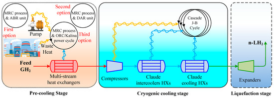
Figure 1.
The schematic of the three scenarios considered for improving the performance of the H2 liquefaction process using waste energy.
Detailed data are presented in Appendix A: Table A1 lists the operating characteristics of the flow involved in different scenarios, including temperature, pressure, molar enthalpy, molar entropy, mass flow rate, and exergy rate. Table A2 outlines the equipment’s input, output, and exergy destruction characteristics in various scenarios. Figure A1 shows the exergy destruction contribution of the equipment used in different scenarios (ABR-, DAR-, and ORC/Kalina-based units).
Figure 2 depicts the block flow diagram (BFD) of the H2 liquefaction process by implementing the ammonia–water ABR cycle. Figure 3 depicts the process flow diagram (PFD) of the H2 liquefaction process by implementing the ammonia–water ABR cycle.
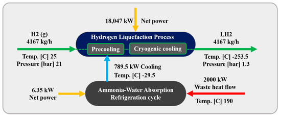
Figure 2.
Block flow diagram of the H2 liquefaction process by implementing the ammonia–water absorption refrigeration cycle.
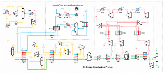
Figure 3.
Process flow diagram of the hydrogen liquefaction process by implementing the ammonia–water absorption refrigeration cycle.
3.1. Process Description
The H2 liquefaction process begins with hydrogen entering the system as stream H1 at 2100 kPa and 25 °C. It passes through a series of heat exchangers, HX6, HX7, and HX8, progressively reducing its temperature. After passing through the HX6 exchangers, the hydrogen is cooled to −45 °C; after the HX7 exchangers, to −105 °C; and after the HX8 exchangers, to −195 °C at stream H4. In this process, H2 exists in two isomeric forms: ortho-H2, where the H2 molecules have parallel spins, and para-H2, which has antiparallel spins. The conversion from ortho- to para-H2 is important because para-H2 has lower thermal energy and a lower boiling point, making it more suitable for liquefaction. Following the heat exchangers, the H2 moves through two conversion reactors (CR1 and CR2), where the para-H2 concentration increases. Three types of reactors, including isothermal, adiabatic, and continuous converters, can be used for ortho- to para-H2 conversion in simulation studies [14]. In this study, two isothermal reactors (CR1 and CR2) and a continuous conversion unit integrated into the HX13 heat exchanger are applied to perform the conversion process. The feed stream entering the hydrogen liquefaction system contains ortho-H2 at 25 °C and 21 bar. The ortho- to para-H2 conversion is an exothermic and temperature-dependent reaction. This reaction is essential in liquid hydrogen production for long-distance transportation because it helps reduce boil-off gas losses [46]. Based on the extracted experimental data [47], the para-hydrogen concentration is set to 49.71% at the outlet of thermal reactor CR1 and 94.18% at the outlet of CR2. A catalyst-based tubular heat exchanger is employed to reach a 99.9% para-H2 concentration at a temperature of −253 °C. In this configuration, CR2 is positioned upstream of HX13, which finalizes the subcooling stage before expansion. Both CR1 and CR2 are modeled as idealized reactors (isothermal or adiabatic), which simplifies the simulation while preserving the thermodynamic intent of the process. The H2 pressure remains at 2100 kPa, so the T7 turboexpander is used to lower the pressure to 130 kPa, preparing the H2 for storage and transportation. The thermodynamic modeling of H2 flow and refrigeration cycles within the integrated system is carried out using the modified Benedict–Webb–Rubin (MBWR) and Peng–Robinson equations of state in Aspen HYSYS V10 [6,48].
3.1.1. Precooling Stage
In the precooling phase, the multi-component refrigerant stream (i.e., flow L7) enters the D2 flash drum, separating it into liquid and vapor phases. These phases are then directed to the HX6 heat exchanger, which supplies part of the cooling needed to reduce the H2’s temperature to −45 °C. A similar process occurs with stream L10. After passing through the HX6, HX7, and HX8 heat exchangers, the gaseous phases of the refrigerant streams flow into the T1, T2, and T3 turbo expanders to reduce pressure. The expanded gases are subsequently combined through the M1 and M2 mixers. The returning stream (i.e., stream L24) undergoes two compression stages and is cooled to 25 °C before entering mixer M7 and proceeding back to the D2 flash drum to complete the cycle.
3.1.2. Claude Cryogenic Refrigeration Cycle
The cascade Joule–Brayton cycle in the developed hybrid structure includes three Claude processes. The Claude cryogenic refrigeration cycle reduces the H2 temperature further to −239.5 °C. The Claude cycle, known for its appropriate thermodynamic efficiency, is extensively utilized in large-scale liquefaction facilities and effectively handles a variety of gases, including hydrogen, helium, nitrogen, oxygen, and natural gas. This cycle operates with a mixed refrigerant consisting of H2, helium, and neon. It captures heat from the H2 stream using the HX9, HX11, and HX13 heat exchangers. After the refrigerant streams are collected in the M4 mixer, the combined stream (i.e., flow L26) undergoes three compression stages in the C3, C4, and C5 compressors, raising its pressure from 1 to 1000 kPa. After compression, the stream is cooled in the HX1, HX2, and HX3 heat exchangers to stabilize at 25 °C.
At this stage, stream L47 under 25 °C and 1000 kPa is divided into three separate streams: L32, L33, and L34. These streams pass through the HX10, HX12, and HX14 heat exchangers, followed by the T4, T5, and T6 turbo expanders, which lower the streams’ pressure and temperature. These cooled streams then provide the necessary cryogenic cooling for hydrogen in the HX9, HX11, and HX13 heat exchangers.
3.2. Ammonia–Water Absorption Refrigeration Cycle (First Scenario)
In this scenario, an ammonia–water ABR cycle is integrated to contribute to the precooling phase of the H2 liquefaction process. The system harnesses 2000 kW of waste heat from an external unit, which is directed to the generator to separate the ammonia from water. The ABR process operates using the fundamental principles of absorption refrigeration and includes critical components such as the evaporator, absorber, generator, and condenser. In this cycle, ammonia is absorbed into the water at low pressure, and then ammonia vapor is released at higher pressure, generating the cooling effect required. This makes the ABR particularly suitable for industrial settings with access to waste heat, providing an energy-efficient solution for large-scale refrigeration processes. The BFD and the PFD of the ABR-based H2 liquefaction process are illustrated in Figure 2 and Figure 3, respectively.
In the ABR cycle, the liquid ammonia stream (i.e., flow W12) enters the HX6 heat exchanger at −29.55 °C and 120 kPa, exiting at −29.50 °C. This process provides 789.4 kW of cooling duty for the H2 precooling stage. After passing through the H17 heat exchanger, the stream (i.e., stream W13), including a mixture of ammonia and water, enters the absorber. In the absorption process, ammonia is absorbed into water in the M5 mixer. The resulting stream (i.e., flow W1), containing 0.74 mol% ammonia and 0.26 mol% water, undergoes adjustments in temperature and pressure before entering the generator (simulated as a distillation tower, DT) at 126.7 °C and 1300 kPa (i.e., stream W6). In the generator, ammonia is separated from the water, with the gaseous ammonia (i.e., stream W17) exiting from the top of the distillation tower. The ammonia is then condensed in the HX16 heat exchanger, reducing its temperature to −29.55 °C. After lowering its pressure to 120 kPa using the V1 expansion valve, the liquid ammonia is directed back to the HX6 heat exchanger, which provides the necessary cooling for the H2 precooling stage.
3.3. Diffusion Absorption Refrigeration Cycle (Second Scenario)
In this scenario, a DAR Cycle is employed to support the precooling stage of the H2 liquefaction process. The DAR cycle leverages absorption refrigeration principles enhanced by a diffusion process. Helium is the refrigerant, diffusing through a porous medium and mixing with an ammonia–water absorbent solution. This diffusion improves the absorption of the refrigerant, boosting the system’s overall efficiency. Figure 4 and Figure 5 present the BFD and PFD for the DAR process involved in the liquid H2 cycle. The system utilizes water, ammonia, and helium as working fluids and includes two main subsystems: distillation columns DT1 and DT2, which are essential for effective heat management. The DT2 column functions as a generator, reservoir, and bubble pump within the cycle. The system’s single-pressure configuration eliminates mechanical pumps, relying on the thermosyphon effect, which enhances energy efficiency and increases system reliability. The system utilizes 2000 kW of waste heat from an external source to power the generator in the DT2 column, further contributing to its energy efficiency.
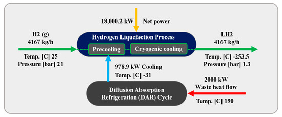
Figure 4.
Process flow diagram of the hydrogen liquefaction process implementing the diffusion absorption refrigeration cycle.
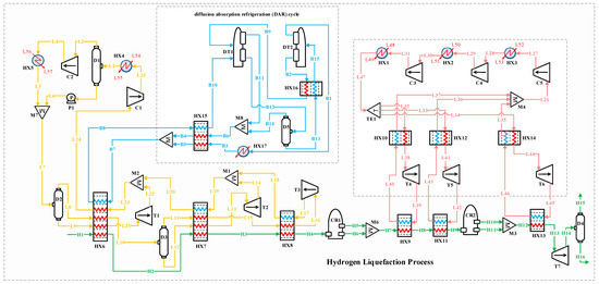
Figure 5.
Process flow diagram of the hydrogen liquefaction process by implementing the diffusion absorption refrigeration cycle.
The DAR process includes various equipment and processes, as explained below.
- Heat exchange and vaporization: The concentrated ammonia–water solution (i.e., stream B15) enters the DT2 column, where it is preheated by a weaker ammonia–water solution coming from the bubble pump output. This heat input vaporizes the ammonia, creating a vapor mixture of ammonia and water.
- Separation in the rectifier: In the DT2’s rectifier, the ammonia vapor is condensed, separating it into pure ammonia vapor (i.e., stream B1), while the water condensate returns to the generator by gravity. The ammonia vapor undergoes a phase change into liquid, releasing heat through an exothermic process.
- Precooling with helium: After being cooled to 2 °C in the HX17 and HX15 heat exchangers, the liquid ammonia (i.e., stream B5) is mixed with helium (i.e., stream B4). The resulting mixture (i.e., stream B7) enters the HX6 heat exchanger at −31.7 °C and 2500 kPa, providing 978.9 kW of cooling to precool the H2 during liquefaction. Stream B8 exits the HX6 heat exchanger at −5.85 °C and then passes through the HX15 heat exchanger before entering the DT1 tower at 24.05 °C.
- Absorption in DT1 column: In DT1, the absorber mixes stream B10 (a preheated ammonia-helium mixture from the HX15 heat exchanger) with stream B9 (a precooled weak ammonia–water solution from the HX16 heat exchanger). This forms a strong ammonia–water solution (i.e., stream B12), which exits the absorber while releasing heat to the environment.
- Helium recovery: Helium is extracted from the top of the DT1 tower and the D5 drum (i.e., streams B11 and B14), and these are collected in the M8 mixer for recirculation within the cycle.
The system is modeled using the Peng–Robinson equation of state in Aspen HYSYS V10, ensuring accurate thermodynamic property predictions for the ABR and DAR processes.
3.4. Combination of Organic Rankine and Kalina Power Cycles (Third Scenario)
In this scenario, the ORC and Kalina cycles are combined within the H2 liquefaction process to recover 2000 kW of waste heat. This recovered heat is used to generate power for the precooling stage. Both thermodynamic cycles effectively convert the waste heat into mechanical energy, which is then transformed into electrical power, supplying a portion of the energy needed for liquefaction. The BFD and PFD for the combined ORC/Kalina power cycle are shown in Figure 6 and Figure 7, respectively.

Figure 6.
Block flow diagram of the hydrogen liquefaction process using the combination of ORC/Kalina power generation cycle.
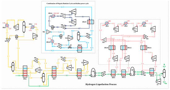
Figure 7.
Process flow diagram of the hydrogen liquefaction process using the combination of ORC and Kalina power generation cycle.
3.4.1. Organic Rankine Cycle Process Description
R-290 is selected as the working fluid for the ORC system due to its good thermodynamic properties for low- to medium-temperature waste heat recovery. It has a low boiling point of −42 °C, high latent heat of vaporization, favorable pressure ratios, and good thermal stability, making it highly efficient in ORC applications. Moreover, R-290 is a natural refrigerant with zero ozone depletion potential (ODP) and very low global warming potential (GWP = 3), making it an environmentally friendly choice compared to synthetic refrigerants. Its widespread availability, low cost, and proven performance in both refrigeration and power generation cycles further support its suitability in this study [49]. The ORC cycle involves several pieces of equipment and processes, which are detailed below:
- Heat absorption: In this process, stream R1, initially at 30.0 °C and 2500 kPa, enters the HX16 heat exchanger and absorbs 2000 kW of heat, exiting at 178.7 °C (i.e., stream R2).
- Power generation: Stream R2 splits into two streams, R3 and R5, which enter the T8 and T9 turbines, respectively, for power generation. The T8 turbine reduces the pressure to 1500 kPa, generating 220.1 kW of power. Also, the T9 turbine generates 21.77 kW by reducing the pressure of stream R5.
- Heat transfer to Kalina cycle: Stream R4 transfers 1786.2 kW of heat to the Kalina cycle via the HX15 heat exchanger, cooling from 125.1 to 7.23 °C (i.e., stream R7).
3.4.2. Kalina Power Cycle Process Description
As an adaptation of the Rankine cycle, the Kalina power cycle uses an ammonia–water mixture to optimize heat energy utilization under varying heat source temperatures. The waste heat from the ORC cycle is recovered through integration with the Kalina cycle, leading to an improvement in the overall system efficiency. The Kalina cycle involves several equipment and processes, which are detailed below.
- Ammonia–water solution heating: A rich ammonia–water solution (i.e., stream K12) enters the flash drum at 96.66 °C and 2290 kPa, where ammonia vapor is separated and directed to the T10 turbine for power generation.
- Power generation: the T10 turbine lowers the pressure from 2280 kPa (i.e., stream K13) to 450 kPa (i.e., stream K15), producing 245.2 kW of power.
- Absorption and pressure recovery: After the turbine, the ammonia vapor is absorbed into the weak ammonia–water solution (i.e., stream K17) in the M9 mixer, forming stream K18. This stream is pumped to 2300 kPa by the P3 pump, consuming 6.14 kW of electrical power to complete the cycle.
- Energy integration: The total net electrical power generated in this scenario contributes to the electricity required for the precooling stage in the H2 liquefaction process, enhancing system efficiency by utilizing waste heat to generate part of the necessary energy.
The simulation is performed using Aspen HYSYS V10 with the Peng–Robinson equation of state, ensuring accurate thermodynamic property calculations for the ORC and Kalina systems.
4. Simulation Methodology
Aspen HYSYS V10 is coupled with the m-file in MATLAB programming to simulate the three scenarios for the H2 liquefaction process. This integration facilitates the design of the complex, integrated process while allowing for comprehensive analyses, including energy and exergy evaluations. These analyses are crucial for assessing the process’s overall performance and its subsystems’ efficiency. The following assumptions are made for the simulations:
- Kinetic and potential energy changes in the process streams are considered negligible. This simplification assumes that these energy contributions are insignificant compared to the thermal and mechanical energy flows involved in the process.
- All streams are assumed to be in a steady-state condition, meaning their properties (temperature, pressure, flow rates) remain constant over time.
- Pressure drops and heat losses in the heat exchangers are ignored. This assumes ideal behavior in heat exchangers, focusing on their thermal performance without accounting for inefficiencies due to pressure losses or external heat leakage.
- The pumps and turbines in the system are modeled using isentropic efficiency, representing the ratio of actual work to the ideal (isentropic) work. This ensures realistic performance modeling while simplifying mechanical work and heat interaction calculation.
4.1. Energy Analysis
Energy analysis involves quantitatively assessing the inflow and outflow of energy within a system. It relies on the principles outlined in the first law of thermodynamics. The equation for steady-state control volume energy and mass balance, derived from the first law of thermodynamics, is as follows [50]:
in which represents the total work, denotes the mass flow rate, refers to the net heat transfer rate, z indicates the elevation from a reference position, is the specific enthalpy, corresponds to the stream velocity of the working fluid, and signifies the gravitational acceleration. Equation (2) presents the energy balance in heat exchangers [19].
Isentropic efficiency is presumed within the energy balance equations governing compressors and pumps (Equation (3)) and turbines (Equation (4)), disregarding heat loss. Thus, the energy balance for such equipment is [19]:
Within the mixer, energy balance and mass conservation equations are as follows [19]:
In separators and flash drums, the same procedure as a mixer can be considered [19] as follows:
According to the first law of thermodynamics, the enthalpy remains unchanged during the throttling process within valves. Consequently [19], the following applies:
The SPC and the COP are important design parameters for assessing system performance quality. The specific power consumption of the system is calculated as follows [42]:
The overall COP measures the amount of cooling generated per unit of system power consumption, articulated as follows [42]:
In this equation, denotes the total net power used in the process, refers to feed H2 gas, represents the mass flow rate of the liquid H2, is the mass enthalpy of feed gas H2 and represents the mass enthalpy of produced liquid H2.
Figure 8, depicting the comprehensive balance within one of its stages, is used to model the distillation columns, applicable across various design configurations. Each tray sees the entry and exit of both vapor and liquid streams, facilitating the representation of towers featuring multiple feeds, products, and auxiliary heat exchangers. The MESH equations, which include material, equilibrium, summation, and heat balances, can be written as follows [51]:
In this equation, j is the tray number, and i is the component number. W represents the vapor side stream, F represents feed, L stands for liquid fraction, V represents the vapor stream, and U is vapor fraction. The equilibrium equation for every segment within a tray of the tower is as follows:
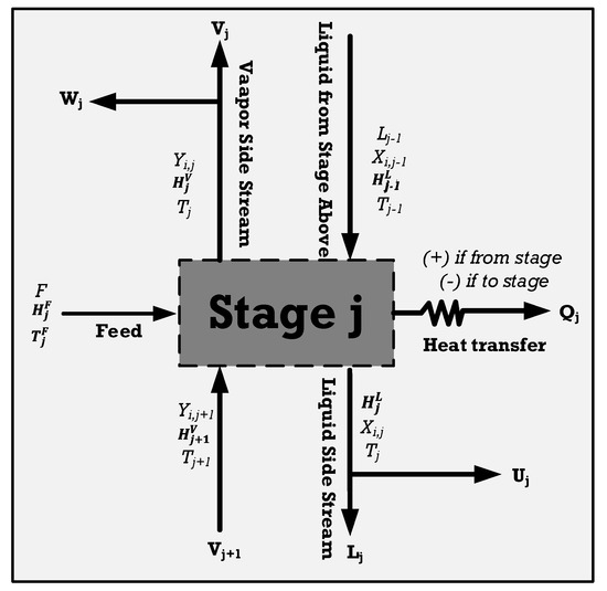
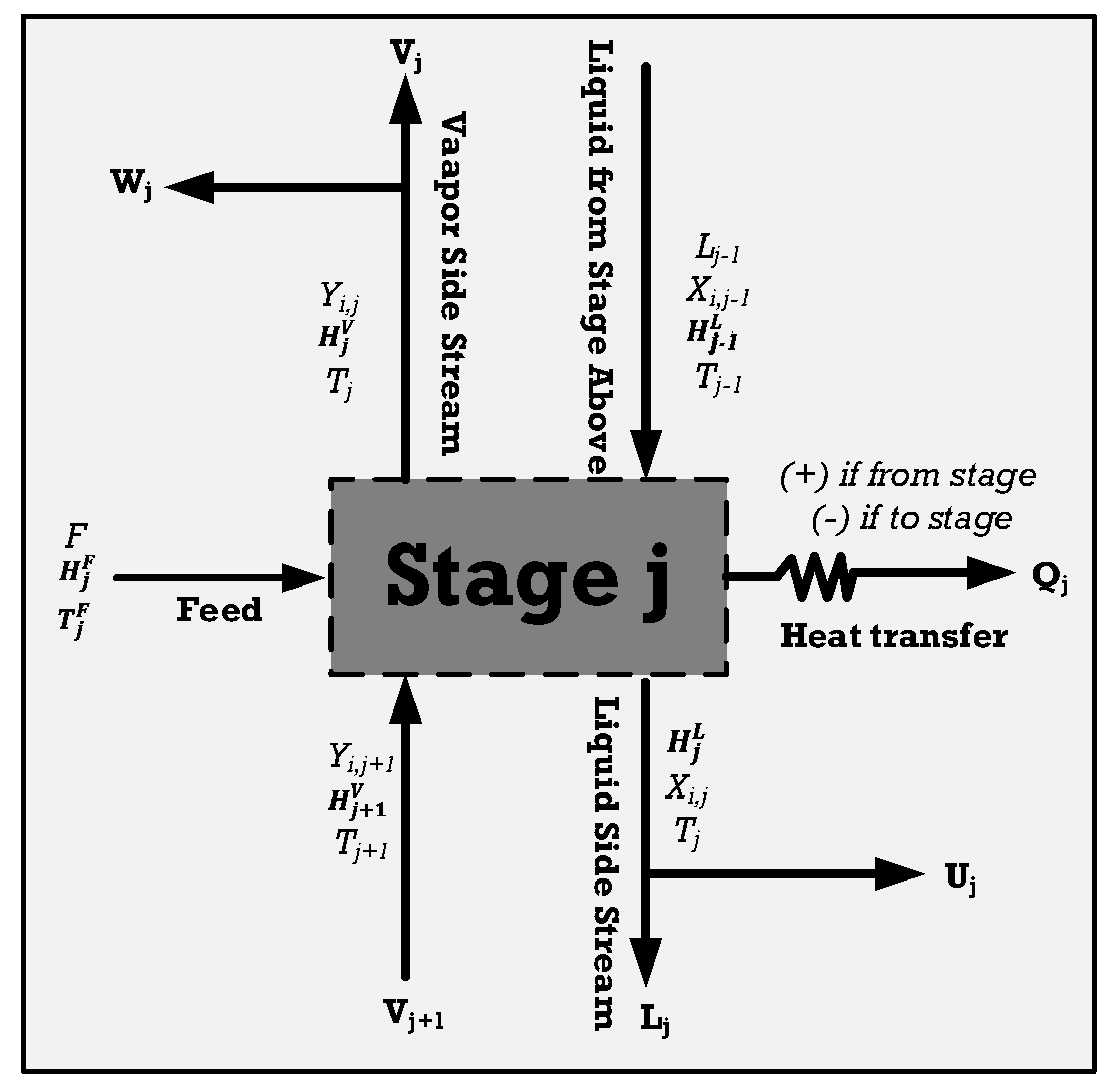
Figure 8.
The overall balance in one of the stages of the tower, modified from [51].
Figure 8.
The overall balance in one of the stages of the tower, modified from [51].
The equation representing the total for every tray is as follows:
The equation describing the thermal energy balance for each tray is:
In this context, H signifies enthalpy, while Qj is calculated according to the temperature of the heat source, denoted as T0.
4.2. Exergy Analysis
Exergy reflects the ability of a unit or apparatus to generate useful work and provides crucial insights into enhancing system efficiency. It assesses how effectively the energy input from equipment or a stream is converted into useful work and the amount lost in the process. Exergy is the maximum work obtainable when a system transitions from a given state to ambient conditions, commonly set at 25 °C and 1 atm pressure, in a reversible process [52].
In essence, exergy is equivalent to reversible work. This refers to the maximum usable work that can be achieved (or the minimum energy consumed in power-consuming equipment) during a process between initial and final states. The primary goal of exergy analysis is to pinpoint locations and causes of exergy destruction. The amount of consumed exergy is referred to as irreversibility or exergy destruction. Thus, the exergy destruction rate is directly linked to the amount of entropy generated [53].
The exergy destruction is always positive in real systems and zero in reversible systems. In cases where kinetic energy, potential energy, nuclear effects, electrical, magnetic, and surface tension effects are negligible, the exergy rate of the entire system can be considered as the sum of the following components [53]:
denotes the exergy rate of the fluid flow, refers to the sum of the physical exergy rate and represents the sum of the chemical exergy rate. The rates of physical exergy and chemical exergy are determined using the following equations [53]:
Here, represents the activity coefficient of the ith component, which can exceed or fall below one, being zero for an ideal mixture of various compounds. and denote the enthalpy and entropy of the flow at ambient temperature and pressure. In an ideal mixture, interactions between molecules are negligible, and the mixture’s properties can be computed solely based on the properties of individual components and their respective proportions. Calculating the chemical exergy of such a nonideal mixture of various compounds becomes intricate due to the presence of the activity coefficient.
It can be demonstrated that the second component of Equation (20) represents the Gibbs free energy alteration caused by the blending of diverse compounds and the creation of a solution under ambient temperature and pressure conditions. Ultimately, the chemical exergy equation undergoes the following transformation [54]:
ΔGmix signifies the Gibbs free energy alteration of the mixture under ambient temperature and pressure conditions. Identifying the distribution and magnitude of irreversibility across different processes within a thermodynamic system is the critical objective of conducting an exergy analysis. This analysis aids in assessing the extent of inefficiencies and devising strategies for enhancing system performance. The exergy balance equation can be expressed as follows [51]:
This equation serves to compute irreversibility or exergy destruction, where and represent the input and output exergies of flows, denotes output exergies of energy flows, signifies the shaft work on or by the system, is input exergy of energy flows, and I indicates irreversibility or exergy destruction [51]:
The equations used for calculating the exergy efficiency and exergy destruction of each equipment and the total process in different scenarios for the liquefaction of hydrogen are provided in Table 1.

Table 1.
Exergy efficiency and destruction formulas of the equipment used in the design [55,56,57].
5. Results and Discussion
The research focuses on industrial waste heat recovery for refrigeration and power generation within H2 liquefaction cycles. The 2 MW recovered heat is utilized in ABR, DAR, and ORC/Kalina power cycles to support precooling in H2 liquefaction cycles. The results of energy, exergy, and validation analyses are presented below.
5.1. Pinch Analysis
Pinch analysis is an effective method for minimizing energy consumption in thermodynamic processes and heat recovery systems. It helps optimize heat exchanger design, reducing the need for external heating and cooling [58]. Temperature gaps always exist between cold and hot streams in multi-stream heat exchangers. The closer the hot and cold streams are in these exchangers, the lower the power consumption of the refrigeration cycle, resulting in a higher overall system efficiency. Pinch technology enables adjustments to energy consumption and determines the necessary utility loads using important tools such as hot and cold composite curves. The pinch points occur due to the limited temperature approach between hot and cold streams, especially in the precooling and cryogenic stages, where small temperature differences are critical for maintaining system efficiency. In this study, Aspen HYSYS V10 software is employed to identify the pinch point, while MATLAB V10 integrated with Aspen HYSYS is used to generate the composite curves. Among the three systems, the DAR-based process exhibited a slightly higher pinch temperature difference due to lower temperature glide and weaker temperature matching between streams, while the ORC/Kalina-based scenario achieved better thermal integration, reducing the pinch effect.
The analysis also shows that heat exchangers are the largest contributors to exergy loss in all three configurations. This is primarily because of unavoidable temperature differences within multi-stream heat exchangers, especially when handling fluids with varying specific heat capacities and phase-change behavior. The large surface areas required and high heat duty intensify irreversible processes, particularly in the cryogenic precooling stage. Improving heat exchanger design, such as by minimizing the temperature approach and optimizing stream allocation, is essential to reduce these losses and enhance overall system performance.
Figure 9 shows the hot and cold composite curves of the complex heat exchanger network designed for the H2 liquefaction process.
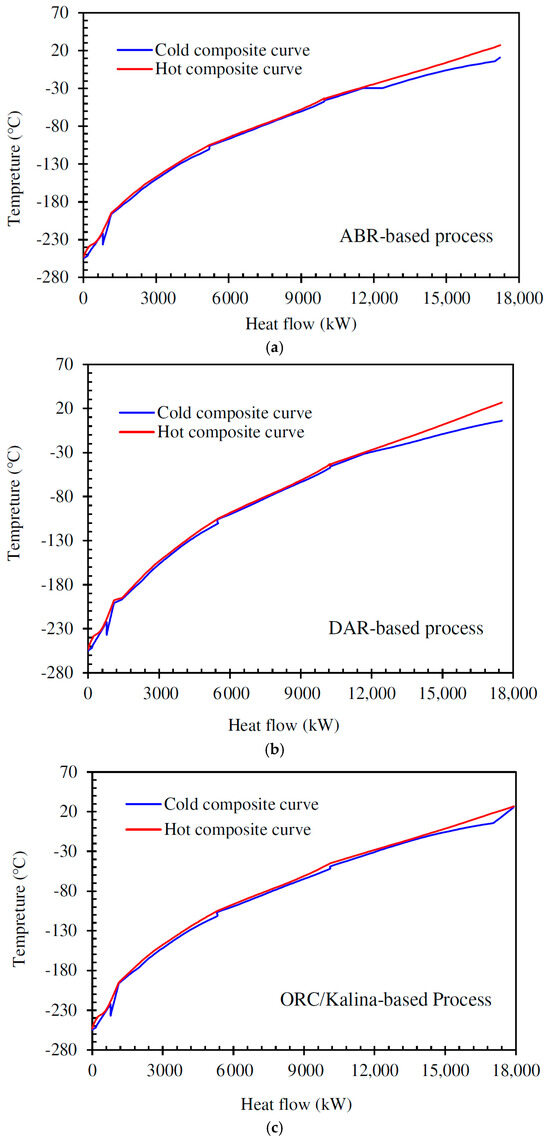
Figure 9.
Cold and hot composite curves for the process using (a) the ammonia–water absorption refrigeration cycle, (b) the diffusion absorption refrigeration cycle, (c) the combination of ORC and Kalina power generation cycle.
5.2. Exergy Analysis Results
To begin the exergy analysis, the first step is to calculate the exergy of the streams within the processes and assess the exergy destruction for each component. The exergy destruction and efficiency are determined by applying the exergy balance to individual equipment components. Table 2 illustrates each equipment group’s contribution to the total exergy destruction in the different scenarios. Heat exchangers account for the majority of exergy destruction, with 48% in both the DAR- and ORC/Kalina-based scenarios and 47% in the ABR-based process. Turbines account for approximately 21–22% of the total exergy destruction. Across all scenarios, pumps have the lowest contribution to exergy destruction.
Table 2.
The share of each piece of equipment in total exergy destruction.
Table 3 summarizes the total exergy efficiency and destruction for the various scenarios and their subsystems. The data indicate that both the overall integrated process and the exergy efficiency of the H2 precooling process have improved compared to the basic cycle. The ABR-based cycle achieves the highest total exergy efficiency at 52.47%, followed by the ORC/Kalina-based cycle at 51.45%. The DAR-based cycle exhibits the lowest total exergy efficiency, at 51.28%.
Table 3.
Comparison between the key parameters related to the performance of different scenarios considered in the hydrogen liquefaction process.
In the H2 precooling process, the ORC/Kalina-based scenario demonstrates the highest exergy efficiency at 70.84%, followed by the DAR-based and ABR-based cycles at 69.72% and 68.85%, respectively. The H2 cryogenic unit’s exergy efficiency is equal for the ORC/Kalina- and DAR-based scenarios at 51.65%, matching the basic process. However, the ABR-based cycle achieves a higher efficiency of 53.31%. Also, the exergy efficiency of the diffusion absorption refrigeration subsystem in the DAR-based scenario is 24.85%, while the absorption refrigeration subsystem in the ABR-based scenario has an efficiency of 23.69%. Regarding exergy destruction, the ORC/Kalina-based scenario records the lowest exergy destruction at 8.03 MW, followed by the ABR-based scenario at 8.07 MW and the DAR-based scenario at 8.30 MW.
5.3. Comparison and Validation Analyses
Figure 10 illustrates the comparison of SPC among the developed scenarios in this study compared to reference [46]. The results show that the ORC/Kalina-based scenario achieved the lowest SPC at 4.306 kWh/kg LH2, followed by the DAR-based scenario at 4.320 kWh/kg LH2, and the ABR-based scenario at 4.333 kWh/kg LH2, with the ORC/Kalina scenario slightly outperforming the others. These differences in SPC are attributed to variations in the specific power of the multi-component refrigeration processes utilized during the precooling stage. While the SPC of the cascaded Joule–Brayton subsystem is nearly identical across all three scenarios, at around 3.425 kWh/kg LH2 the SPC of the multi-component refrigeration unit mirrors the overall SPC trends for the different scenarios. Therefore, the mixed refrigerant refrigeration cycle in the ORC/Kalina-based scenario records the lowest value among all scenarios at 0.882 kWh/kg LH2, compared to 0.896 kWh/kg LH2 for the DAR-based scenario and 0.907 kWh/kg LH2 for the ABR-based scenario.
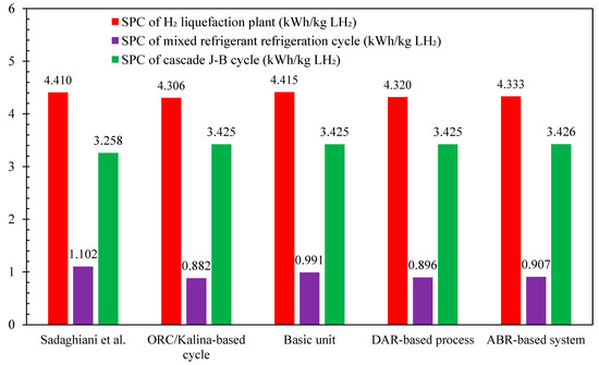
Figure 10.
Comparison of the specific power consumption values for the developed scenarios in this study and reference [46].
Table 4 compares the COP of the liquefaction process and the exergy efficiencies of its subsystems across the different scenarios under study and reference [46]. The COP for all scenarios are nearly identical, measuring 0.286, which is 2% higher than the basic unit and nearly 60% higher than the values reported in reference [46]. Figure 11 compares the required power consumption, exergy destruction, and SPC of the H2 liquefaction system across the various scenarios under study. Table 5 presents a comparison of the COP of the cryogenic unit, the SPC of the precooling process, and the exergy efficiencies of both the overall and liquefaction processes across the different scenarios under study. The total power consumption for the designed H2 liquefaction processes, operating at a rate of 4167 kg/h, is calculated to be 17.94 MW for the ORC/Kalina-based scenario, 18 MW for the DAR-based scenario, and 18.05 MW for the ABR-based scenario.
Table 4.
The comparison between the COP of the liquefaction process and the exergy efficiencies of its subsystems in the different scenarios in this study and reference [46].
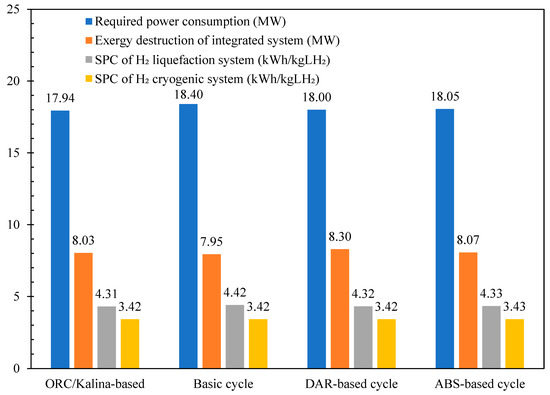
Figure 11.
The comparison between the required power consumptions, exergy destructions, and SPC of the hydrogen liquefaction system in the different scenarios in this study.
Table 5.
The comparison between the COP of the cryogenic unit, SPC of the precooling process, and exergy efficiencies of the whole and the liquefaction processes in the different scenarios under study.
Table A3 shows the key operational results of the H2 liquefaction units proposed in this work relative to previously published data. It is important to highlight that the SPC values reported in this study, such as 4.306 kWh/kgLH2 for the ORC/Kalina-based scenario, are lower than those reported in some literature. This discrepancy derives primarily from the model’s assumptions, which include steady-state operation, neglect of pressure losses, perfect thermal integration, and the ideal behavior of heat exchangers and components. Also, the waste heat integration strategy is optimized under the assumption of full recovery potential. As such, the results presented herein represent a theoretical lower bound on SPC achievable under idealized conditions. While this provides insight into the thermodynamic potential of different system configurations, practical implementations are expected to yield higher energy consumption. Future work should incorporate detailed component-level losses and experimental validations to bridge this gap between theory and practice.
Figure 12 compares the scenarios based on ORC/Kalina and DAR integration with the hydrogen liquefaction cycle against the results from reference [36]. The results demonstrate that the ORC/Kalina-based liquefaction process for heat recovery has higher SPC and COP rates compared to other scenarios developed in this study and reference [36]. Table 6 presents the validation of the simulated DAR cycle in this paper against the cycle designed in reference [36]. The COP and exergy efficiency of the DAR cycle developed in this study are calculated as 0.4893 and 0.2485, respectively, with a difference of less than 1% compared to the values reported in the reference. The simulations conducted in this study demonstrate a satisfactory alignment with the critical design parameters reported in the reference literature.

Figure 12.
The validation results of the different scenarios with reference paper [36].
Table 6.
Validation result of the DAR-based scenario compared to reference paper [36].
6. Conclusions
Improving the energy efficiency of H2 liquefaction remains a critical challenge due to its high power consumption and thermodynamic limitations. This study introduces a novel approach by systematically evaluating the integration of waste heat recovery into the liquefaction cycle through three innovative scenarios. Unlike previous studies that focus on isolated efficiency improvements, this work comprehensively examines and compares the effectiveness of three distinct waste heat utilization strategies, each leveraging 2 MW of excess industrial heat to optimize liquefaction performance:
- Ammonia–Water Absorption Refrigeration Cycle: uses waste heat to drive an absorption-based precooling system, reducing reliance on electrical refrigeration.
- Diffusion Absorption Refrigeration Cycle: employs a single-pressure absorption cooling system powered by waste heat to enhance H2 precooling.
- Organic Rankine and Kalina Power Cycles: converts waste heat into electricity, reducing external energy demands for liquefaction.
The most significant contributions and findings of this study are as follows:
- Energy Efficiency Gains: The ORC/Kalina-based system demonstrated the lowest SPC at 4.306 kWh/kg LH2, outperforming the DAR-based (4.320 kWh/kg LH2) and ABR-based (4.333 kWh/kg LH2) methods. All scenarios improved the COP by approximately 2% over the baseline, showing a significant efficiency advantage over previous studies. Pinch analysis confirmed optimized energy integration across all cases.
- Exergy optimization: Exergy analysis identified heat exchangers as the dominant source of exergy destruction, contributing nearly 50% of the total irreversible processes. Among the proposed methods, the ORC/Kalina cycle achieved the highest exergy efficiency for hydrogen precooling (70.84%), while the ABR-based system exhibited the highest overall exergy efficiency (52.47%). These results provide critical insights into the thermodynamic limitations of hydrogen liquefaction and the role of waste heat recovery in mitigating losses.
- Impact on Hydrogen Liquefaction Technology: The ORC/Kalina scenario emerged as the most energy-efficient solution regarding SPC and exergy destruction, whereas the ABR-based cycle achieved the highest overall exergy efficiency. These findings validate the feasibility of integrating industrial waste heat into hydrogen liquefaction, establishing a scalable and practical framework for reducing operational costs and enhancing sustainability.
- Based on the detailed energy and exergy analyses, the three H2 liquefaction scenarios can be ranked as follows:
- ORC/Kalina-based scenario: best performance in terms of energy efficiency, with the lowest SPC (4.306 kWh/kg LH2) and highest exergy efficiency in the precooling unit (70.84%).
- DAR-based scenario: slightly higher SPC (4.320 kWh/kg LH2) and competitive exergy efficiency (precooling unit at 69.83%), with a balanced performance.
- ABR-based scenario—highest SPC (4.333 kWh/kg LH2) but the best overall exergy efficiency (52.47%), making it favorable from a thermodynamic optimization perspective.
This ranking highlights a performance trade-off: the ORC/Kalina-based system is the most energy-efficient, while the ABR cycle offers superior thermodynamic sustainability. The choice between them may depend on specific project priorities- minimizing energy consumption versus maximizing exergy efficiency.
This study provides a comprehensive foundation for the next generation of energy-efficient H2 liquefaction systems, bridging the gap between thermodynamic modeling and real-world implementation. Future work should explore economic feasibility and sensitivity analyses to evaluate cost-effectiveness and determine whether the added complexity of integrating waste heat recovery justifies the efficiency gains. The economic evaluation of the process can be conducted using the annualized cost of the structure method, which provides a realistic estimate of the annual financial burden and makes it easier to compare different configurations or technologies on a consistent economic basis. Key parameters considered in this evaluation include the payback period, net annual benefit, and the prime cost of electricity. This method supports a comprehensive economic assessment and enhances decision-making in selecting the most cost-effective and sustainable process design.
Author Contributions
Conceptualization, S.M.B. and A.I.; Methodology, S.M.B. and A.A.A.; Software, S.M.B.; Formal analysis, A.I., A.A.A. and D.R.R.; Investigation, S.M.B., A.I., A.A.A. and D.R.R.; Writing—original draft, S.M.B. and A.I.; Writing—review & editing, A.I. and D.R.R.; Supervision, A.I.; Project administration, D.R.R. All authors have read and agreed to the published version of the manuscript.
Funding
This research was funded by NSERC Discovery Grant—RGPIN/4220-2019 (for Adrian Ilinca).
Data Availability Statement
The original contributions presented in this study are included in the article. Further inquiries can be directed to the corresponding author.
Acknowledgments
During the preparation of this work, the author(s) did not use generative AI technologies. The authors used AI-assisted technologies, Grammarly (www.grammarly.com (accessed on 10 March 2025) and Antidote (www.antidote.info (accessed on 10 March 2025), to improve formulation and eliminate grammatical errors. After using this tool/service, the author(s) reviewed and edited the content as needed and take(s) full responsibility for the publication’s content.
Conflicts of Interest
The authors declare no conflict of interest.
Appendix A
Table A1 lists the operating characteristics of the flow involved in different scenarios, including temperature, pressure, molar enthalpy, molar entropy, mass flow rate, and exergy rate. Table A2 outlines the equipment’s input, output, and exergy destruction characteristics in various scenarios. Table A3 compares the key outcome parameters of the H2 liquefaction systems developed in this study with those reported in the literature. Figure A1 shows the exergy destruction contribution of the equipment used in different scenarios (ABR-, DAR-, and ORC/Kalina-based units).
Table A1.
The operating characteristics of the flow across different scenarios.
Table A1.
The operating characteristics of the flow across different scenarios.
| ABR-Based Process | ||||||
| Stream | Temperature (°C) | Pressure (kPa) | Molar Enthalpy (kJ/kmol) | Molar Entropy (kJ/kmol °C) | Mass Flow (kg/h) | Exergy (kW) |
| L1 | 25.0 | 700.0 | −124,459.3 | 163.8 | 100,833.3 | 994,814.1 |
| L2 | 25.0 | 700.0 | −121,010.2 | 171.1 | 86,958.8 | 810,201.2 |
| L3 | 25.0 | 700.0 | −161,438.5 | 85.0 | 13,874.6 | 184,612.9 |
| L4 | 69.6 | 1600.0 | −118,732.6 | 171.8 | 86,958.8 | 811,506.7 |
| L5 | 25.0 | 1600.0 | −123,476.7 | 156.8 | 86,958.8 | 811,340.6 |
| L6 | 25.4 | 1600.0 | −161,329.6 | 85.0 | 13,874.6 | 184,618.4 |
| L7 | 27.0 | 1600.0 | −126,706.1 | 150.7 | 100,833.3 | 995,946.4 |
| L8 | 27.0 | 1600.0 | −120,790.4 | 164.5 | 71,711.5 | 613,094.1 |
| L9 | 27.0 | 1600.0 | −150,858.4 | 94.4 | 29,121.8 | 382,852.2 |
| L10 | −43.0 | 1600.0 | −129,599.4 | 130.9 | 71,711.5 | 613,756.7 |
| L11 | −43.0 | 1600.0 | −128,504.1 | 152.8 | 42,051.9 | 250,363.8 |
| L12 | −43.0 | 1600.0 | −131,716.1 | 88.7 | 29,659.6 | 363,392.9 |
| L13 | −105.0 | 1600.0 | −137,147.2 | 61.3 | 29,659.6 | 363,906.3 |
| L14 | −107.7 | 200.0 | −137,239.7 | 61.4 | 29,659.6 | 363,885.4 |
| L15 | −105.0 | 1600.0 | −136,127.8 | 113.8 | 42,051.9 | 251,820.4 |
| L16 | −195.0 | 1600.0 | −143,755.2 | 52.1 | 42,051.9 | 255,726.0 |
| L17 | −196.4 | 200.0 | −143,824.7 | 52.2 | 42,051.9 | 255,689.9 |
| L18 | −110.5 | 200.0 | −132,654.2 | 146.3 | 42,051.9 | 249,559.1 |
| L19 | −106.1 | 200.0 | −134,217.7 | 117.5 | 71,711.5 | 613,411.0 |
| L20 | −47.5 | 200.0 | −125,625.4 | 161.8 | 71,711.5 | 610,877.4 |
| L21 | −45.0 | 1600.0 | −160,283.0 | 58.6 | 29,121.8 | 383,018.5 |
| L22 | −49.3 | 200.0 | −160,434.8 | 58.7 | 29,121.8 | 382,995.0 |
| L23 | −46.2 | 200.0 | −132,474.0 | 141.5 | 100,833.3 | 993,864.8 |
| L24 | 11.1 | 200.0 | −123,018.6 | 178.4 | 100,833.3 | 992,798.6 |
| L25 | 70.7 | 700.0 | −119,525.4 | 179.5 | 100,833.3 | 994,987.9 |
| L26 | 23.5 | 100.0 | −32.6 | 92.8 | 41,804.6 | 87,029.2 |
| L27 | 138.8 | 215.4 | 2420.3 | 93.4 | 41,804.6 | 91,801.5 |
| L28 | 25.0 | 215.4 | −1.0 | 86.5 | 41,804.6 | 91,024.2 |
| L29 | 140.8 | 464.2 | 2464.3 | 87.1 | 41,804.6 | 95,822.7 |
| L30 | 25.0 | 464.2 | −2.2 | 80.1 | 41,804.6 | 95,019.3 |
| L31 | 140.8 | 1000.0 | 2463.3 | 80.7 | 41,804.6 | 99,818.1 |
| L32 | 25.0 | 1000.0 | −4.6 | 73.7 | 8151.9 | 19,307.8 |
| L33 | 25.0 | 1000.0 | −4.6 | 73.7 | 20,693.3 | 49,012.2 |
| L34 | 25.0 | 1000.0 | −4.6 | 73.7 | 12,959.4 | 30,694.5 |
| L35 | 23.9 | 100.0 | −23.8 | 92.8 | 12,959.4 | 26,979.0 |
| L36 | 23.4 | 100.0 | −35.3 | 92.8 | 20,693.3 | 43,079.5 |
| L37 | 23.2 | 100.0 | −39.5 | 92.8 | 8151.9 | 16,970.7 |
| L38 | −194.0 | 1000.0 | −4676.4 | 45.4 | 8151.9 | 20,851.9 |
| L39 | −236.5 | 100.0 | −5562.7 | 48.3 | 8151.9 | 20,138.5 |
| L40 | −196.5 | 100.0 | −4711.3 | 64.0 | 8151.9 | 18,569.2 |
| L41 | −219.0 | 1000.0 | −5216.4 | 37.2 | 20,693.3 | 54,912.1 |
| L42 | −248.2 | 100.0 | −5813.1 | 40.0 | 20,693.3 | 53,412.2 |
| L43 | −221.7 | 100.0 | −5247.1 | 55.5 | 20,693.3 | 49,207.5 |
| L44 | −245.0 | 1000.0 | −5792.6 | 22.7 | 12,959.4 | 36,835.8 |
| L45 | −255.0 | 100.0 | −6128.0 | 24.8 | 12,959.4 | 36,208.0 |
| L46 | −248.2 | 100.0 | −5811.9 | 40.1 | 12,959.4 | 33,441.6 |
| L47 | 25.0 | 1000.0 | −4.6 | 73.7 | 41,804.6 | 99,014.6 |
| L48 | 24.0 | 101.1 | −285,672.3 | 55.2 | 60,153.9 | 10,861.3 |
| L49 | 99.0 | 101.1 | −280,190.8 | 71.6 | 60,153.9 | 11,397.9 |
| L50 | 24.0 | 101.1 | −285,672.3 | 55.2 | 61,276.5 | 11,064.0 |
| L51 | 99.0 | 101.1 | −280,190.8 | 71.6 | 61,276.5 | 11,610.6 |
| L52 | 24.0 | 101.1 | −285,672.3 | 55.2 | 61,309.3 | 11,069.9 |
| L53 | 99.0 | 101.1 | −280,190.8 | 71.6 | 61,309.3 | 11,616.8 |
| L54 | 24.0 | 101.1 | −285,672.3 | 55.2 | 143,763.8 | 25,957.8 |
| L55 | 45.0 | 101.1 | −284,143.8 | 60.2 | 143,763.8 | 26,061.0 |
| L56 | 24.0 | 101.1 | −285,672.3 | 55.2 | 102,123.8 | 18,439.3 |
| L57 | 50.0 | 101.1 | −283,779.9 | 61.3 | 102,123.8 | 18,552.8 |
| H1 | 25.0 | 2100.0 | 8475.5 | 116.9 | 4166.7 | 141,251.6 |
| H2 | −45.0 | 2100.0 | 6472.0 | 109.2 | 4166.7 | 141,411.6 |
| H3 | −105.0 | 2100.0 | 4822.9 | 100.9 | 4166.7 | 141,898.4 |
| H4 | −195.0 | 2100.0 | 2579.5 | 81.9 | 4166.7 | 143,853.9 |
| H5 | −195.0 | 2100.0 | 2291.9 | 81.8 | 4166.6 | 143,156.1 |
| H7 | −195.0 | 2100.0 | 2291.9 | 81.8 | 4166.6 | 143,156.2 |
| H8 | −219.0 | 2100.0 | 1684.8 | 72.5 | 4166.6 | 144,402.0 |
| H9 | −239.5 | 2100.0 | 660.2 | 47.3 | 4166.6 | 148,118.3 |
| H10 | −240.0 | 2100.0 | −120.6 | 28.4 | 4166.4 | 147,975.8 |
| H12 | −240.0 | 2100.0 | −120.6 | 28.4 | 4166.4 | 149,483.0 |
| H13 | −253.0 | 2100.0 | −479.0 | 15.2 | 4166.4 | 151,540.9 |
| H14 | −253.5 | 130.0 | −528.2 | 15.5 | 4166.4 | 151,464.5 |
| H16 | −253.5 | 130.0 | −528.2 | 15.5 | 4166.4 | 151,464.5 |
| W1 | 54.1 | 120.0 | −225,213.2 | 80.6 | 14,356.9 | 21,783.8 |
| W2 | 31.9 | 120.0 | −230,824.9 | 62.9 | 14,356.9 | 21,713.3 |
| W3 | 25.0 | 200.0 | −285,010.9 | 6.6 | 217,182.2 | 39,220.1 |
| W4 | 30.0 | 190.0 | −284,634.6 | 7.9 | 217,182.2 | 39,229.9 |
| W5 | 32.0 | 1300.0 | −230,796.6 | 62.9 | 14,356.9 | 21,719.5 |
| W6 | 126.7 | 1300.0 | −222,020.6 | 87.5 | 14,356.9 | 22,038.7 |
| W7 | 104.2 | 1300.0 | −55,230.4 | 159.0 | 3869.5 | 20,614.8 |
| W8 | 37.0 | 1300.0 | −271,521.7 | 59.2 | 11,485.5 | 5862.2 |
| W9 | 37.3 | 120.0 | −271,521.7 | 59.2 | 11,485.5 | 5857.8 |
| W10 | 34.0 | 1300.0 | −66,320.8 | 83.9 | 2871.4 | 16,224.7 |
| W11 | −24.5 | 1300.0 | −71,072.1 | 66.7 | 2871.4 | 16,241.2 |
| W12 | −29.6 | 120.0 | −71,072.1 | 66.9 | 2871.4 | 16,239.0 |
| W13 | −29.5 | 120.0 | −54,214.6 | 136.1 | 2871.4 | 16,062.3 |
| W14 | 154.9 | 1300.0 | −248,032.3 | 87.1 | 14,754.1 | 12,917.7 |
| W15 | 25.0 | 200.0 | −285,010.9 | 6.6 | 164,951.3 | 29,787.9 |
| W16 | 30.0 | 190.0 | −284,634.6 | 7.9 | 164,951.3 | 29,795.4 |
| W17 | 45.5 | 1300.0 | −45,883.0 | 150.3 | 2871.4 | 16,253.6 |
| W18 | 173.9 | 1300.0 | −260,433.7 | 88.7 | 11,485.5 | 6268.0 |
| W19 | −29.3 | 120.0 | −49,463.3 | 155.6 | 2871.4 | 16,012.6 |
| DAR-Based Process | ||||||
| Stream | Temperature (°C) | Pressure (kPa) | Molar Enthalpy (kJ/kmol) | Molar Entropy (kJ/kmol °C) | Mass Flow (kg/h) | Exergy (kW) |
| L1 | 25.0 | 700.0 | −124,459.3 | 163.8 | 100,833.3 | 994,814.1 |
| L2 | 25.0 | 700.0 | −121,010.2 | 171.1 | 86,958.8 | 810,201.2 |
| L3 | 25.0 | 700.0 | −161,438.5 | 85.0 | 13,874.6 | 184,612.9 |
| L4 | 69.6 | 1600.0 | −118,732.6 | 171.8 | 86,958.8 | 811,506.7 |
| L5 | 25.0 | 1600.0 | −123,476.7 | 156.8 | 86,958.8 | 811,340.6 |
| L6 | 25.4 | 1600.0 | −161,329.6 | 85.0 | 13,874.6 | 184,618.4 |
| L7 | 27.0 | 1600.0 | −126,706.1 | 150.7 | 100,833.3 | 995,946.4 |
| L8 | 27.0 | 1600.0 | −120,790.4 | 164.5 | 71,711.5 | 613,094.1 |
| L9 | 27.0 | 1600.0 | −150,858.4 | 94.4 | 29,121.8 | 382,852.2 |
| L10 | −43.0 | 1600.0 | −129,599.4 | 130.9 | 71,711.5 | 613,756.7 |
| L11 | −43.0 | 1600.0 | −128,504.1 | 152.8 | 42,051.9 | 250,363.8 |
| L12 | −43.0 | 1600.0 | −131,716.1 | 88.7 | 29,659.6 | 363,392.9 |
| L13 | −105.0 | 1600.0 | −137,147.2 | 61.3 | 29,659.6 | 363,906.3 |
| L14 | −107.7 | 200.0 | −137,239.7 | 61.4 | 29,659.6 | 363,885.4 |
| L15 | −105.0 | 1600.0 | −136,127.8 | 113.8 | 42,051.9 | 251,820.4 |
| L16 | −195.0 | 1600.0 | −143,755.2 | 52.1 | 42,051.9 | 255,726.0 |
| L17 | −196.4 | 200.0 | −143,824.7 | 52.2 | 42,051.9 | 255,689.9 |
| L18 | −110.5 | 200.0 | −132,654.2 | 146.3 | 42,051.9 | 249,559.1 |
| L19 | −106.1 | 200.0 | −134,217.7 | 117.5 | 71,711.5 | 613,411.0 |
| L20 | −47.5 | 200.0 | −125,625.4 | 161.8 | 71,711.5 | 610,877.4 |
| L21 | −45.0 | 1600.0 | −160,283.0 | 58.6 | 29,121.8 | 383,018.5 |
| L22 | −49.3 | 200.0 | −160,434.8 | 58.7 | 29,121.8 | 382,995.0 |
| L23 | −46.2 | 200.0 | −132,474.0 | 141.5 | 100,833.3 | 993,864.8 |
| L24 | 6.4 | 200.0 | −123,294.4 | 177.5 | 100,833.3 | 992,809.5 |
| L25 | 65.8 | 700.0 | −119,860.8 | 178.5 | 100,833.3 | 994,958.8 |
| L26 | 23.1 | 100.0 | −40.1 | 92.8 | 41,804.6 | 87,029.3 |
| L27 | 138.3 | 215.4 | 2410.0 | 93.4 | 41,804.6 | 91,795.5 |
| L28 | 25.0 | 215.4 | −1.0 | 86.5 | 41,804.6 | 91,024.2 |
| L29 | 140.8 | 464.2 | 2464.3 | 87.1 | 41,804.6 | 95,822.7 |
| L30 | 25.0 | 464.2 | −2.2 | 80.1 | 41,804.6 | 95,019.3 |
| L31 | 140.8 | 1000.0 | 2463.3 | 80.7 | 41,804.6 | 99,818.1 |
| L32 | 25.0 | 1000.0 | −4.6 | 73.7 | 8151.9 | 19,307.8 |
| L33 | 25.0 | 1000.0 | −4.6 | 73.7 | 20,693.3 | 49,012.2 |
| L34 | 25.0 | 1000.0 | −4.6 | 73.7 | 12,959.4 | 30,694.5 |
| L35 | 23.9 | 100.0 | −23.8 | 92.8 | 12,959.4 | 26,979.0 |
| L36 | 22.6 | 100.0 | −50.5 | 92.7 | 20,693.3 | 43,079.6 |
| L37 | 23.2 | 100.0 | −39.5 | 92.8 | 8151.9 | 16,970.7 |
| L38 | −194.0 | 1000.0 | −4676.4 | 45.4 | 8151.9 | 20,851.9 |
| L39 | −236.5 | 100.0 | −5562.7 | 48.3 | 8151.9 | 20,138.5 |
| L40 | −196.5 | 100.0 | −4711.3 | 64.0 | 8151.9 | 18,569.2 |
| L41 | −219.0 | 1000.0 | −5216.4 | 37.2 | 20,693.3 | 54,912.1 |
| L42 | −248.2 | 100.0 | −5813.1 | 40.0 | 20,693.3 | 53,412.2 |
| L43 | −222.4 | 100.0 | −5262.3 | 55.2 | 20,693.3 | 49,283.9 |
| L44 | −245.0 | 1000.0 | −5792.6 | 22.7 | 12,959.4 | 36,835.8 |
| L45 | −255.0 | 100.0 | −6128.0 | 24.8 | 12,959.4 | 36,208.0 |
| L46 | −248.2 | 100.0 | −5811.9 | 40.1 | 12,959.4 | 33,441.6 |
| L47 | 25.0 | 1000.0 | −4.6 | 73.7 | 41,804.6 | 99,014.6 |
| L48 | 24.0 | 101.1 | −285,672.3 | 55.2 | 59,897.8 | 10,815.0 |
| L49 | 99.0 | 101.1 | −280,190.8 | 71.6 | 59,897.8 | 11,349.3 |
| L50 | 24.0 | 101.1 | −285,672.3 | 55.2 | 61,276.5 | 11,064.0 |
| L51 | 99.0 | 101.1 | −280,190.8 | 71.6 | 61,276.5 | 11,610.6 |
| L52 | 24.0 | 101.1 | −285,672.3 | 55.2 | 61,309.3 | 11,069.9 |
| L53 | 99.0 | 101.1 | −280,190.8 | 71.6 | 61,309.3 | 11,616.8 |
| L54 | 24.0 | 101.1 | −285,672.3 | 55.2 | 133,990.4 | 24,193.1 |
| L55 | 45.0 | 101.1 | −284,143.8 | 60.2 | 133,990.4 | 24,289.3 |
| L56 | 24.0 | 101.1 | −285,672.3 | 55.2 | 102,123.8 | 18,439.3 |
| L57 | 50.0 | 101.1 | −283,779.9 | 61.3 | 102,123.8 | 18,552.8 |
| H1 | 25.0 | 2100.0 | 8475.5 | 116.9 | 4166.7 | 141,251.6 |
| H2 | −45.0 | 2100.0 | 6472.0 | 109.2 | 4166.7 | 141,411.6 |
| H3 | −105.0 | 2100.0 | 4822.9 | 100.9 | 4166.7 | 141,898.4 |
| H4 | −195.0 | 2100.0 | 2579.5 | 81.9 | 4166.7 | 143,853.9 |
| H5 | −195.0 | 2100.0 | 2291.9 | 81.8 | 4166.6 | 143,156.1 |
| H7 | −195.0 | 2100.0 | 2291.9 | 81.8 | 4166.6 | 143,156.2 |
| H8 | −219.0 | 2100.0 | 1684.8 | 72.5 | 4166.6 | 144,402.0 |
| H9 | −239.0 | 2100.0 | 687.7 | 48.1 | 4166.6 | 147,995.2 |
| H10 | −240.0 | 2100.0 | −82.8 | 30.3 | 4166.4 | 147,737.2 |
| H12 | −240.0 | 2100.0 | −82.8 | 30.4 | 4166.4 | 149,242.0 |
| H13 | −253.0 | 2100.0 | −441.2 | 17.1 | 4166.4 | 151,299.8 |
| H14 | −253.5 | 130.0 | −490.4 | 17.4 | 4166.4 | 151,223.5 |
| H16 | −253.5 | 130.0 | −490.4 | 17.4 | 4166.4 | 151,223.5 |
| B1 | 65.3 | 2500.0 | −45,671.5 | 145.8 | 2999.3 | 17,038.4 |
| B2 | 188.5 | 2500.0 | −243,856.7 | 93.8 | 8927.4 | 8217.1 |
| B3 | 35.0 | 2500.0 | −66,040.8 | 84.1 | 2999.3 | 16,941.9 |
| B4 | −3.1 | 2500.0 | −1574.4 | 57.3 | 10,285.3 | 29,030.7 |
| B5 | 2.0 | 2500.0 | −68,794.1 | 74.7 | 2999.3 | 16,945.0 |
| B6 | 22.3 | 2500.0 | −992.8 | 59.3 | 10,285.3 | 29,009.3 |
| B7 | −31.7 | 2500.0 | −6108.0 | 58.8 | 13,284.7 | 45,900.9 |
| B8 | −5.8 | 2500.0 | −4761.2 | 64.2 | 13,284.7 | 45,717.0 |
| B9 | 43.0 | 2500.0 | −255,907.2 | 62.6 | 8927.4 | 7837.3 |
| B10 | 24.1 | 2500.0 | −4033.1 | 66.8 | 13,284.7 | 45,686.8 |
| B11 | 22.3 | 2500.0 | −992.8 | 59.3 | 10,285.2 | 29,008.8 |
| B12 | 25.3 | 2500.0 | −209,227.5 | 63.6 | 11,927.4 | 24,492.9 |
| B13 | 21.8 | 2500.0 | −209,511.7 | 62.7 | 11,927.3 | 24,492.7 |
| B14 | 21.8 | 2500.0 | −3383.5 | 65.3 | 0.2 | 0.5 |
| B15 | 128.0 | 2500.0 | −200,608.3 | 88.3 | 11,927.3 | 24,728.0 |
| ORC/Kalina-Based Process | ||||||
| Stream | Temperature (°C) | Pressure (kPa) | Molar Enthalpy (kJ/kmol) | Molar Entropy (kJ/kmol °C) | Mass Flow (kg/h) | Exergy (kW) |
| L1 | 25.0 | 700.0 | −124,459.3 | 163.8 | 106,775.5 | 1,053,439.5 |
| L2 | 25.0 | 700.0 | −121,010.2 | 171.1 | 92,083.3 | 857,947.2 |
| L3 | 25.0 | 700.0 | −161,438.5 | 85.0 | 14,692.2 | 195,492.3 |
| L4 | 69.6 | 1600.0 | −118,732.6 | 171.8 | 92,083.3 | 859,329.6 |
| L5 | 25.0 | 1600.0 | −123,476.7 | 156.8 | 92,083.3 | 859,153.7 |
| L6 | 25.4 | 1600.0 | −161,329.6 | 85.0 | 14,692.2 | 195,498.2 |
| L7 | 27.0 | 1600.0 | −126,706.1 | 150.7 | 106,775.5 | 1,054,638.5 |
| L8 | 27.0 | 1600.0 | −120,790.4 | 164.5 | 75,937.5 | 649,224.4 |
| L9 | 27.0 | 1600.0 | −150,858.4 | 94.4 | 30,838.0 | 405,414.1 |
| L10 | −45.0 | 1600.0 | −129,863.2 | 129.8 | 75,937.5 | 649,972.4 |
| L11 | −45.0 | 1600.0 | −128,689.4 | 152.3 | 43,520.3 | 254,850.5 |
| L12 | −45.0 | 1600.0 | −132,006.7 | 88.7 | 32,417.2 | 395,122.0 |
| L13 | −105.0 | 1600.0 | −137,225.8 | 62.3 | 32,417.2 | 395,672.0 |
| L14 | −108.0 | 200.0 | −137,319.3 | 62.3 | 32,417.2 | 395,648.8 |
| L15 | −105.0 | 1600.0 | −136,037.8 | 114.5 | 43,520.3 | 256,329.9 |
| L16 | −195.0 | 1600.0 | −143,727.0 | 52.4 | 43,520.3 | 260,408.2 |
| L17 | −196.4 | 200.0 | −143,796.7 | 52.5 | 43,520.3 | 260,370.6 |
| L18 | −111.4 | 200.0 | −132,695.0 | 146.4 | 43,520.3 | 253,998.0 |
| L19 | −106.8 | 200.0 | −134,331.3 | 116.9 | 75,937.5 | 649,612.2 |
| L20 | −51.6 | 200.0 | −126,115.6 | 159.6 | 75,937.5 | 646,972.6 |
| L21 | −45.0 | 1600.0 | −160,283.0 | 58.6 | 30,838.0 | 405,590.1 |
| L22 | −49.3 | 200.0 | −160,434.8 | 58.7 | 30,838.0 | 405,565.2 |
| L23 | −48.8 | 200.0 | −132,867.7 | 139.8 | 106,775.5 | 1,052,526.3 |
| L24 | 25.7 | 200.0 | −122,144.0 | 181.4 | 106,775.5 | 1,051,290.8 |
| L25 | 86.1 | 700.0 | −118,468.1 | 182.5 | 106,775.5 | 1,053,740.4 |
| L26 | 23.1 | 100.0 | −40.1 | 92.8 | 41,804.6 | 87,029.3 |
| L27 | 138.3 | 215.4 | 2410.0 | 93.4 | 41,804.6 | 91,795.5 |
| L28 | 25.0 | 215.4 | −1.0 | 86.5 | 41,804.6 | 91,024.2 |
| L29 | 140.8 | 464.2 | 2464.3 | 87.1 | 41,804.6 | 95,822.7 |
| L30 | 25.0 | 464.2 | −2.2 | 80.1 | 41,804.6 | 95,019.3 |
| L31 | 140.8 | 1000.0 | 2463.3 | 80.7 | 41,804.6 | 99,818.1 |
| L32 | 25.0 | 1000.0 | −4.6 | 73.7 | 8151.9 | 19,307.8 |
| L33 | 25.0 | 1000.0 | −4.6 | 73.7 | 20,693.3 | 49,012.2 |
| L34 | 25.0 | 1000.0 | −4.6 | 73.7 | 12,959.4 | 30,694.5 |
| L35 | 23.9 | 100.0 | −23.8 | 92.8 | 12,959.4 | 26,979.0 |
| L36 | 22.6 | 100.0 | −50.5 | 92.7 | 20,693.3 | 43,079.6 |
| L37 | 23.2 | 100.0 | −39.5 | 92.8 | 8151.9 | 16,970.7 |
| L38 | −194.0 | 1000.0 | −4676.4 | 45.4 | 8151.9 | 20,851.9 |
| L39 | −236.5 | 100.0 | −5562.7 | 48.3 | 8151.9 | 20,138.5 |
| L40 | −196.5 | 100.0 | −4711.3 | 64.0 | 8151.9 | 18,569.2 |
| L41 | −219.0 | 1000.0 | −5216.4 | 37.2 | 20,693.3 | 54,912.1 |
| L42 | −248.2 | 100.0 | −5813.1 | 40.0 | 20,693.3 | 53,412.2 |
| L43 | −222.4 | 100.0 | −5262.3 | 55.2 | 20,693.3 | 49,283.9 |
| L44 | −245.0 | 1000.0 | −5792.6 | 22.7 | 12,959.4 | 36,835.8 |
| L45 | −255.0 | 100.0 | −6128.0 | 24.8 | 12,959.4 | 36,208.0 |
| L46 | −248.2 | 100.0 | −5811.9 | 40.1 | 12,959.4 | 33,441.6 |
| L47 | 25.0 | 1000.0 | −4.6 | 73.7 | 41,804.6 | 99,014.6 |
| L48 | 24.0 | 101.1 | −285,672.3 | 55.2 | 59,897.8 | 10,815.0 |
| L49 | 99.0 | 101.1 | −280,190.8 | 71.6 | 59,897.8 | 11,349.3 |
| L50 | 24.0 | 101.1 | −285,672.3 | 55.2 | 61,276.5 | 11,064.0 |
| L51 | 99.0 | 101.1 | −280,190.8 | 71.6 | 61,276.5 | 11,610.6 |
| L52 | 24.0 | 101.1 | −285,672.3 | 55.2 | 61,309.3 | 11,069.9 |
| L53 | 99.0 | 101.1 | −280,190.8 | 71.6 | 61,309.3 | 11,616.8 |
| L54 | 24.0 | 101.1 | −285,672.3 | 55.2 | 149,309.7 | 26,959.1 |
| L55 | 50.0 | 101.1 | −283,779.9 | 61.3 | 149,309.7 | 27,125.1 |
| L56 | 24.0 | 101.1 | −285,672.3 | 55.2 | 108,142.1 | 19,526.0 |
| L57 | 50.0 | 101.1 | −283,779.9 | 61.3 | 108,142.1 | 19,646.2 |
| H1 | 25.0 | 2100.0 | 8475.5 | 116.9 | 4166.7 | 141,251.6 |
| H2 | −45.0 | 2100.0 | 6472.0 | 109.2 | 4166.7 | 141,411.6 |
| H3 | −105.0 | 2100.0 | 4822.9 | 100.9 | 4166.7 | 141,898.4 |
| H4 | −195.0 | 2100.0 | 2579.5 | 81.9 | 4166.7 | 143,853.9 |
| H5 | −195.0 | 2100.0 | 2291.9 | 81.8 | 4166.6 | 143,156.1 |
| H7 | −195.0 | 2100.0 | 2291.9 | 81.8 | 4166.6 | 143,156.2 |
| H8 | −219.0 | 2100.0 | 1684.8 | 72.5 | 4166.6 | 144,402.0 |
| H9 | −239.0 | 2100.0 | 687.7 | 48.1 | 4166.6 | 147,995.2 |
| H10 | −240.0 | 2100.0 | −82.8 | 30.3 | 4166.4 | 147,737.2 |
| H12 | −240.0 | 2100.0 | −82.8 | 30.4 | 4166.4 | 149,242.0 |
| H13 | −253.0 | 2100.0 | −441.2 | 17.1 | 4166.4 | 151,299.8 |
| H14 | −253.5 | 130.0 | −490.4 | 17.4 | 4166.4 | 151,223.5 |
| H16 | −253.5 | 130.0 | −490.4 | 17.4 | 4166.4 | 151,223.5 |
| R1 | 30.0 | 5000.0 | −120,789.5 | 208.4 | 12,258.7 | 167,476.4 |
| R2 | 178.7 | 5000.0 | −94,877.3 | 277.9 | 12,258.7 | 167,879.0 |
| R3 | 178.7 | 5000.0 | −94,877.3 | 277.9 | 11,155.4 | 152,769.9 |
| R4 | 125.1 | 1500.0 | −98,009.3 | 278.7 | 11,155.4 | 152,531.4 |
| R5 | 178.7 | 5000.0 | −94,877.3 | 277.9 | 1103.3 | 15,109.1 |
| R6 | 125.1 | 1500.0 | −98,009.3 | 278.7 | 1103.3 | 15,085.5 |
| R7 | 7.2 | 1500.0 | −123,427.3 | 200.4 | 11,155.4 | 152,386.9 |
| R8 | 26.6 | 1500.0 | −121,139.7 | 208.3 | 12,258.7 | 167,453.3 |
| K1 | 100.0 | 2300.0 | −89,095.0 | 130.3 | 5609.0 | 25,966.3 |
| K2 | 96.7 | 2290.0 | −89,701.4 | 128.7 | 6469.2 | 30,051.1 |
| K3 | 96.5 | 2280.0 | −47,712.7 | 151.4 | 4207.0 | 23,495.6 |
| K4 | 96.5 | 2280.0 | −169,886.9 | 85.3 | 2262.2 | 6554.8 |
| K5 | 19.5 | 450.0 | −51,289.0 | 152.8 | 4207.0 | 23,222.4 |
| K6 | 21.3 | 2270.0 | −175,754.5 | 67.5 | 2262.2 | 6533.9 |
| K7 | 21.7 | 450.0 | −175,754.5 | 67.7 | 2262.2 | 6532.3 |
| K8 | 28.2 | 450.0 | −94,065.1 | 123.6 | 6469.2 | 29,753.4 |
| K9 | 6.8 | 440.0 | −108,878.4 | 72.0 | 6469.2 | 29,812.6 |
| K10 | 5.5 | 101.3 | −287,022.6 | 50.5 | 70,504.8 | 12,783.3 |
| K11 | 25.0 | 101.3 | −285,599.5 | 55.4 | 70,504.8 | 12,730.3 |
| K12 | 7.2 | 2300.0 | −108,819.6 | 72.0 | 6469.2 | 29,817.9 |
| K13 | 7.2 | 2300.0 | −108,819.6 | 72.0 | 860.3 | 3965.1 |
| K14 | 80.0 | 2290.0 | −93,655.0 | 117.7 | 860.3 | 3983.4 |
| K15 | 7.2 | 2300.0 | −108,819.6 | 72.0 | 5609.0 | 25,852.7 |
Table A2.
The input, output, and exergy destruction characteristics of the equipment used in different scenarios.
Table A2.
The input, output, and exergy destruction characteristics of the equipment used in different scenarios.
| ABR-Based Process | ||||
| Equipment | Input Exergy (kW) | Output Exergy (kW) | Exergy Destruction (kW) | Exergy Efficiency |
| HX1 | 102,662.7 | 102,422.0 | 240.7 | 0.953 |
| HX2 | 106,886.7 | 106,629.9 | 256.8 | 0.950 |
| HX3 | 110,888.0 | 110,631.4 | 256.6 | 0.950 |
| HX4 | 1,020,945.7 | 1020,875.1 | 70.6 | 0.979 |
| HX5 | 829,946.0 | 829,893.4 | 52.6 | 0.982 |
| HX6 | 2,147,301.8 | 2,147,047.6 | 254.2 | 0.796 |
| HX7 | 1,368,579.2 | 1,368,502.6 | 76.7 | 0.970 |
| HX8 | 649,408.7 | 649,139.0 | 269.8 | 0.956 |
| HX9 | 163,294.7 | 162,971.1 | 323.6 | 0.794 |
| HX10 | 37,877.0 | 37,822.6 | 54.4 | 0.966 |
| HX11 | 197,814.2 | 197,325.8 | 488.4 | 0.884 |
| HX12 | 98,219.7 | 97,991.6 | 228.1 | 0.963 |
| HX13 | 185,691.1 | 184,982.5 | 708.6 | 0.744 |
| HX14 | 64,136.2 | 63,814.8 | 321.4 | 0.950 |
| HX15 | 61,004.0 | 60,943.2 | 60.7 | 0.952 |
| HX16 | 46,041.5 | 46,020.0 | 21.5 | 0.978 |
| HX17 | 32,286.9 | 32,253.8 | 33.2 | 0.851 |
| T1 | 383,018.5 | 383,015.5 | 3.0 | 0.872 |
| T2 | 363,906.3 | 363,902.8 | 3.5 | 0.834 |
| T3 | 255,726.0 | 255,715.2 | 10.8 | 0.700 |
| T4 | 20,851.9 | 20,501.4 | 350.6 | 0.509 |
| T5 | 54,912.1 | 54,032.4 | 879.7 | 0.413 |
| T6 | 36,835.8 | 36,426.3 | 409.4 | 0.348 |
| T7 | 151,540.9 | 151,492.7 | 48.1 | 0.370 |
| C1 | 995,197.5 | 994,987.9 | 209.6 | 0.913 |
| C2 | 811,631.8 | 811,506.7 | 125.1 | 0.913 |
| C3 | 92,179.6 | 91,801.5 | 378.1 | 0.927 |
| C4 | 96,200.8 | 95,822.7 | 378.1 | 0.927 |
| C5 | 100,196.2 | 99,818.1 | 378.2 | 0.927 |
| P1 | 184,619.3 | 184,618.4 | 0.8 | 0.869 |
| CR1 | 143,853.9 | 143,158.8 | 695.0 | 0.995 |
| CR2 | 148,118.3 | 147,983.2 | 135.1 | 0.999 |
| D1 | 994,814.1 | 994,814.1 | 0.0 | 1.000 |
| D2 | 995,946.4 | 995,946.4 | 0.0 | 1.000 |
| D3 | 613,756.7 | 613,756.7 | 0.0 | 1.000 |
| D4 | 151,464.5 | 151,464.5 | 0.0 | 1.000 |
| DT | 22,778.9 | 22,521.6 | 257.3 | 0.989 |
| V1 | 16,241.2 | 16,239.0 | 2.1 | 0.679 |
| HX18 | 27,987.5 | 27,900.9 | 86.6 | 0.956 |
| P2 | 21,719.7 | 21,719.5 | 0.2 | 0.969 |
| DAR-Based Process | ||||
| Equipment | Input Exergy (kW) | Output Exergy (kW) | Exergy Destruction (kW) | Exergy Efficiency |
| HX1 | 102,610.5 | 102,373.5 | 237.0 | 0.953 |
| HX2 | 106,886.7 | 106,629.9 | 256.8 | 0.950 |
| HX3 | 110,888.0 | 110,631.4 | 256.6 | 0.950 |
| HX4 | 1,019,151.9 | 1,019,103.4 | 48.5 | 0.985 |
| HX5 | 829,946.0 | 829,893.4 | 52.6 | 0.982 |
| HX6 | 2,176,963.7 | 2,176,713.3 | 250.4 | 0.798 |
| HX7 | 1,368,579.2 | 1,368,502.6 | 76.7 | 0.970 |
| HX8 | 649,408.7 | 649,139.0 | 269.8 | 0.956 |
| HX9 | 163,294.7 | 162,971.1 | 323.6 | 0.794 |
| HX10 | 37,877.0 | 37,822.6 | 54.4 | 0.966 |
| HX11 | 197,814.2 | 197,279.1 | 535.1 | 0.870 |
| HX12 | 98,296.1 | 97,991.7 | 304.5 | 0.951 |
| HX13 | 185,450.1 | 184,741.5 | 708.6 | 0.744 |
| HX14 | 64,136.2 | 63,814.8 | 321.4 | 0.950 |
| HX15 | 91,668.2 | 91,662.5 | 5.7 | 0.811 |
| HX16 | 32,709.8 | 32,565.2 | 144.6 | 0.619 |
| HX17 | 17,038.4 | 16,941.9 | 96.5 | 0.994 |
| T1 | 383,018.5 | 383,015.5 | 3.0 | 0.872 |
| T2 | 363,906.3 | 363,902.8 | 3.5 | 0.834 |
| T3 | 255,726.0 | 255,715.2 | 10.8 | 0.700 |
| T4 | 20,851.9 | 20,501.4 | 350.6 | 0.509 |
| T5 | 54,912.1 | 54,032.4 | 879.7 | 0.413 |
| T6 | 36,835.8 | 36,426.3 | 409.4 | 0.348 |
| T7 | 151,299.8 | 151,251.7 | 48.1 | 0.370 |
| C1 | 995,167.8 | 994,958.8 | 209.0 | 0.911 |
| C2 | 811,631.8 | 811,506.7 | 125.1 | 0.913 |
| C3 | 92,173.6 | 91,795.5 | 378.1 | 0.926 |
| C4 | 96,200.8 | 95,822.7 | 378.1 | 0.927 |
| C5 | 100,196.2 | 99,818.1 | 378.1 | 0.927 |
| P1 | 184,619.3 | 184,618.4 | 0.8 | 0.869 |
| CR1 | 143,853.9 | 143,158.8 | 695.0 | 0.995 |
| CR2 | 147,995.2 | 147,744.5 | 250.7 | 0.998 |
| D1 | 994,814.1 | 994,814.1 | 0.0 | 1.000 |
| D2 | 995,946.4 | 995,946.4 | 0.0 | 1.000 |
| D3 | 613,756.7 | 613,756.7 | 0.0 | 1.000 |
| D4 | 151,223.5 | 151,223.5 | 0.0 | 1.000 |
| DT1 | 53,524.1 | 53,501.7 | 22.4 | 1.000 |
| DT2 | 25,468.1 | 25,255.5 | 212.6 | 0.992 |
| ORC/Kalina-Based Process | ||||
| Equipment | Input Exergy (kW) | Output Exergy (kW) | Exergy Destruction (kW) | Exergy Efficiency |
| HX1 | 102,610.5 | 102,373.5 | 237.0 | 0.953 |
| HX2 | 106,886.7 | 106,629.9 | 256.8 | 0.950 |
| HX3 | 110,888.0 | 110,631.4 | 256.6 | 0.950 |
| HX4 | 1,080,699.5 | 1,080,564.5 | 135.0 | 0.969 |
| HX5 | 878,855.6 | 878,799.9 | 55.7 | 0.982 |
| HX6 | 2,248,416.3 | 2,248,264.9 | 151.4 | 0.877 |
| HX7 | 1,440,996.2 | 1,440,872.9 | 123.3 | 0.953 |
| HX8 | 658,599.0 | 658,260.1 | 338.9 | 0.947 |
| HX9 | 163,294.7 | 162,971.1 | 323.6 | 0.794 |
| HX10 | 37,877.0 | 37,822.6 | 54.4 | 0.966 |
| HX11 | 197,814.2 | 197,279.1 | 535.1 | 0.870 |
| HX12 | 98,296.1 | 97,991.7 | 304.5 | 0.951 |
| HX13 | 185,450.1 | 184,741.5 | 708.6 | 0.744 |
| HX14 | 64,136.2 | 63,814.8 | 321.4 | 0.950 |
| HX15 | 178,384.1 | 178,353.2 | 30.9 | 0.983 |
| HX16 | 168,216.8 | 167,879.0 | 1.0 | 0.998 |
| HX17 | 10,520.0 | 10,517.2 | 2.7 | 0.987 |
| T1 | 405,590.1 | 405,586.9 | 3.2 | 0.872 |
| T2 | 395,672.0 | 395,668.1 | 3.8 | 0.834 |
| T3 | 260,408.2 | 260,396.9 | 11.3 | 0.700 |
| T4 | 20,851.9 | 20,501.4 | 350.6 | 0.509 |
| T5 | 54,912.1 | 54,032.4 | 879.7 | 0.413 |
| T6 | 36,835.8 | 36,426.3 | 409.4 | 0.348 |
| T7 | 151,299.8 | 151,251.7 | 48.1 | 0.370 |
| C1 | 1,053,963.9 | 1,053,740.4 | 223.5 | 0.916 |
| C2 | 859,462.1 | 859,329.6 | 132.5 | 0.913 |
| C3 | 92,173.6 | 91,795.5 | 378.1 | 0.926 |
| C4 | 96,200.8 | 95,822.7 | 378.1 | 0.927 |
| C5 | 100,196.2 | 99,818.1 | 378.1 | 0.927 |
| P1 | 195,499.0 | 195,498.2 | 0.9 | 0.869 |
| CR1 | 143,853.9 | 143,158.8 | 695.0 | 0.995 |
| CR2 | 147,995.2 | 147,744.5 | 250.7 | 0.998 |
| D1 | 1,053,439.5 | 1,053,439.5 | 0.0 | 1.000 |
| D2 | 1,054,638.5 | 1,054,638.5 | 0.0 | 1.000 |
| D3 | 649,972.4 | 649,972.4 | 0.0 | 1.000 |
| D4 | 151,223.5 | 151,223.5 | 0.0 | 1.000 |
| T8 | 152,769.9 | 152,751.5 | 18.4 | 0.923 |
| T9 | 15,109.1 | 15,107.3 | 1.8 | 0.923 |
| T10 | 23,495.6 | 23,467.6 | 28.0 | 0.898 |
| P2 | 167,503.4 | 167,453.3 | 3.8 | 0.860 |
| P3 | 29,818.7 | 29,817.9 | 0.9 | 0.856 |
Table A3.
The key outcome parameters of the H2 liquefaction system proposed in this study compared to references.
Table A3.
The key outcome parameters of the H2 liquefaction system proposed in this study compared to references.
| References | Liquefaction Cycle | SPC (kW/kgLH2 & LNG) | Exergy Efficiency | COP |
|---|---|---|---|---|
| Krasae-In et al. [59] (2014) | MR and J-B | 5.91 | 0.489 | 0.149 |
| Ghorbani et al. [44] (2021) | MR and J-B | 5.46 | 0.494 | 0.138 |
| Bian et al. [60] (2021) | LNG regasification and J-B | 6.60 | 0.47 | - |
| Ghorbani et al. [61] (2022) | LNG regasification and J-B | 4.772 | 0.38 | 0.171 |
| Noh et al. [62] (2022) | LNG regasification MR and J-B | 5.798 | 0.686 | - |
| Faramarzi et al. [63] (2022) | LNG cold energy, MR and J-B | 6.59 | 0.46 | - |
| Kim et al. [64] (2022) | MR | 9.477 | 0.34 | 0.23 |
| Yang et al. [25] (2023) | LNG regasification and J-B | 6.59 | 0.47 | - |
| Taghavi et al. [36] (2024) | DAR, MR and J-B | 4.32 | 0.533 | 0.286 |
| Taghavi et al. [36] (2024) | ORC, MR and J-B | 4.359 | 0.508 | 0.280 |
| In this study (basic cycle) | MR and J-B | 4.415 | 0.5018 | 0.280 |
MR (mixed refrigerant) and J-B (Joule-Brayton).
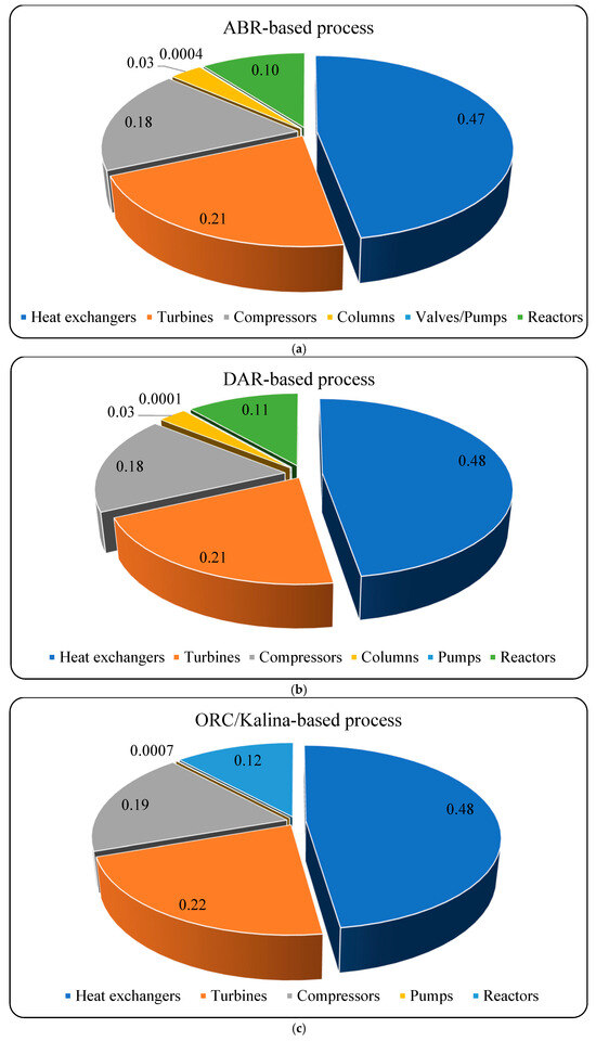
Figure A1.
The exergy destruction contribution of the equipment used in different scenarios: (a) ABR-based process; (b) DAR-based process; (c) ORC/Kalina-based process.
Figure A1.
The exergy destruction contribution of the equipment used in different scenarios: (a) ABR-based process; (b) DAR-based process; (c) ORC/Kalina-based process.
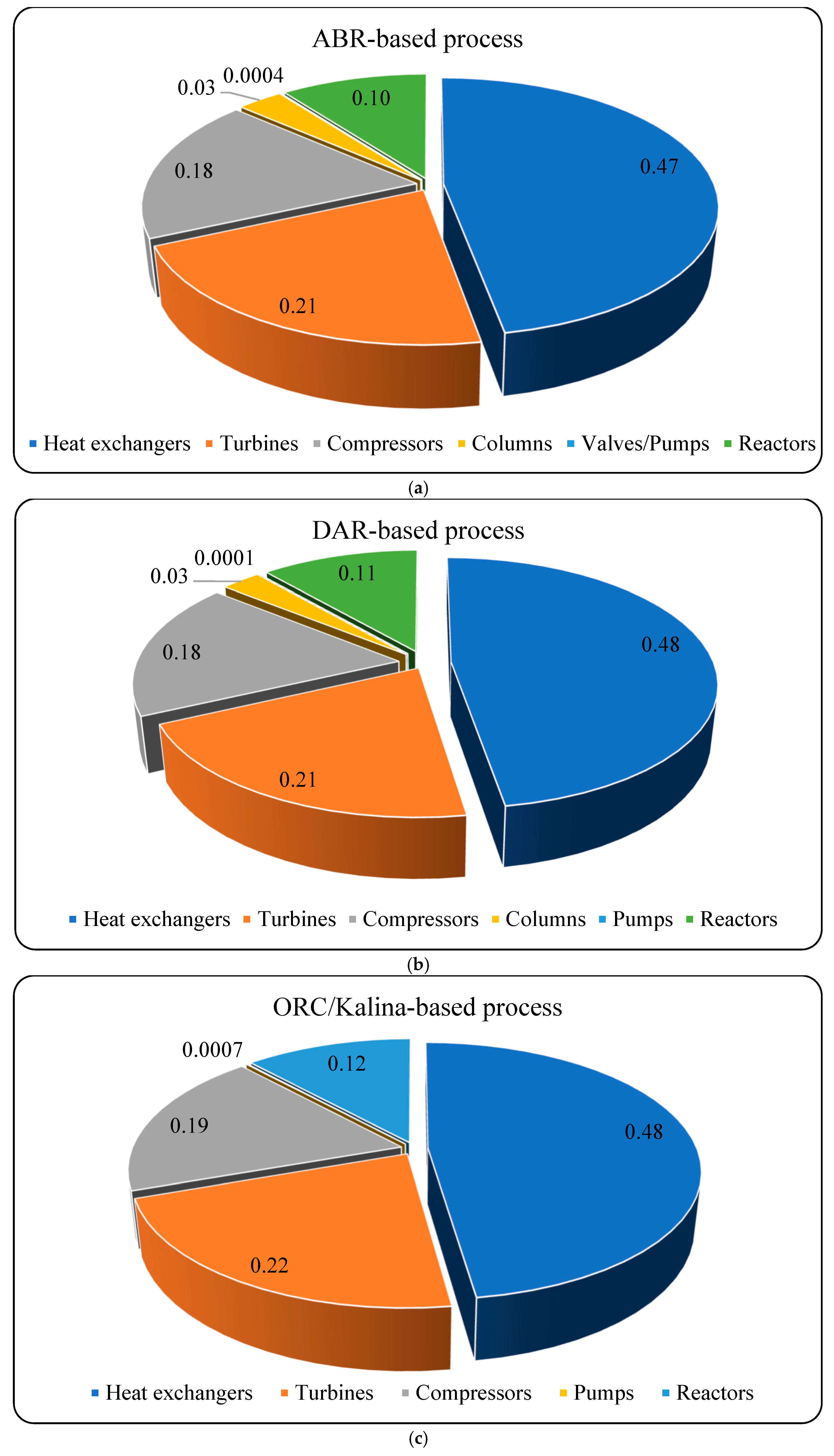
References
- Ghorbani, B.; Zendehboudi, S.; Saady, N.M.C.; Dusseault, M.B. Hydrogen storage in North America: Status, prospects, and challenges. J. Environ. Chem. Eng. 2023, 11, 109957. [Google Scholar] [CrossRef]
- Aasadnia, M.; Mehrpooya, M. Large-scale liquid hydrogen production methods and approaches: A review. Appl. Energy 2018, 212, 57–83. [Google Scholar] [CrossRef]
- Naquash, A.; Qyyum, M.A.; Islam, M.; Sial, N.R.; Min, S.; Lee, S.; Lee, M. Performance enhancement of hydrogen liquefaction process via absorption refrigeration and organic Rankine cycle-assisted liquid air energy system. Energy Convers. Manag. 2022, 254, 115200. [Google Scholar] [CrossRef]
- Al Ghafri, S.Z.; Munro, S.; Cardella, U.; Funke, T.; Notardonato, W.; Trusler, J.M.; Leachman, J.; Span, R.; Kamiya, S.; Pearce, G. Hydrogen liquefaction: A review of the fundamental physics, engineering practice and future opportunities. Energy Environ. Sci. 2022, 15, 2690–2731. [Google Scholar] [CrossRef]
- Ni, M. An overview of hydrogen storage technologies. Energy Explor. Exploit. 2006, 24, 197–209. [Google Scholar]
- Ghorbani, B.; Zendehboudi, S.; Saady, N.M.C.; Azarpour, A.; Albayati, T.M. Thermoeconomic Analysis of an Innovative Integrated System for Cogeneration of Liquid Hydrogen and Biomethane by a Cryogenic-Based Biogas Upgrading Cycle and Polymer Electrolyte Membrane Electrolysis. Ind. Eng. Chem. Res. 2024, 63, 7227–7257. [Google Scholar]
- Rusman, N.; Dahari, M. A review on the current progress of metal hydrides material for solid-state hydrogen storage applications. Int. J. Hydrogen Energy 2016, 41, 12108–12126. [Google Scholar] [CrossRef]
- Taghavi, M.; Salarian, H.; Ghorbani, B. Economic evaluation of a hybrid hydrogen liquefaction system utilizing liquid air cold recovery and renewable energies. Renew. Energy Res. Appl. 2023, 4, 125–143. [Google Scholar]
- Zhang, J.; Fisher, T.S.; Ramachandran, P.V.; Gore, J.P.; Mudawar, I. A review of heat transfer issues in hydrogen storage technologies. ASME J. Heat Mass Transf. 2005, 127, 1391–1399. [Google Scholar]
- Ghorbani, B.; Zendehboudi, S.; Saady, N.M.C.; Duan, X.; Albayati, T.M. Strategies to improve the performance of hydrogen storage systems by liquefaction methods: A comprehensive review. ACS Omega 2023, 8, 18358–18399. [Google Scholar] [CrossRef]
- Kharel, S.; Shabani, B. Hydrogen as a long-term large-scale energy storage solution to support renewables. Energies 2018, 11, 2825. [Google Scholar] [CrossRef]
- Ghorbani, B.; Ebrahimi, A.; Rooholamini, S.; Ziabasharhagh, M. Integrated Fischer-Tropsch synthesis process with hydrogen liquefaction cycle. J. Clean. Prod. 2021, 283, 124592. [Google Scholar] [CrossRef]
- Quack, H. Conceptual Design of a High Efficiency Large Capacity Hydrogen Liquefier; AIP Conference Proceedings; American Institute of Physics: College Park, MD, USA, 2002; pp. 255–263. [Google Scholar]
- Lee, D.; Gbadago, D.Q.; Jo, Y.; Hwang, G.; Jo, Y.; Smith, R.; Hwang, S. Integrating hydrogen liquefaction with steam methane reforming and CO2 liquefaction processes using techno-economic perspectives. Energy Convers. Manag. 2021, 245, 114620. [Google Scholar] [CrossRef]
- Krasae-In, S.; Stang, J.H.; Neksa, P. Simulation on a proposed large-scale liquid hydrogen plant using a multi-component refrigerant refrigeration system. Int. J. Hydrogen Energy 2010, 35, 12531–12544. [Google Scholar] [CrossRef]
- Nouri, M.; Miansari, M.; Ghorbani, B. Exergy and economic analyses of a novel hybrid structure for simultaneous production of liquid hydrogen and carbon dioxide using photovoltaic and electrolyzer systems. J. Clean. Prod. 2020, 259, 120862. [Google Scholar] [CrossRef]
- Riaz, A.; Qyyum, M.A.; Min, S.; Lee, S.; Lee, M. Performance improvement potential of harnessing LNG regasification for hydrogen liquefaction process: Energy and exergy perspectives. Appl. Energy 2021, 301, 117471. [Google Scholar] [CrossRef]
- Qi, M.; Park, J.; Kim, J.; Lee, I.; Moon, I. Advanced integration of LNG regasification power plant with liquid air energy storage: Enhancements in flexibility, safety, and power generation. Appl. Energy 2020, 269, 115049. [Google Scholar] [CrossRef]
- Ghorbani, B.; Zendehboudi, S.; Alizadeh Afrouzi, Z.; Lohi, A.; Khan, F. Efficient Design of the Hydrogen Liquefaction System: Thermodynamic, Economic, Environmental, and Uncertainty Perspectives. Ind. Eng. Chem. Res. 2024, 63, 14668–14699. [Google Scholar] [CrossRef]
- Zendehboudi, S.; Ghorbani, B. Chapter 3—Physical-based hydrogen storage. In Hydrogen Production, Transportation, Storage, and Utilization; Zendehboudi, S., Ghorbani, B., Eds.; Elsevier: Amsterdam, The Netherlands, 2025; pp. 163–253. [Google Scholar] [CrossRef]
- Srikhirin, P.; Aphornratana, S.; Chungpaibulpatana, S. A review of absorption refrigeration technologies. Renew. Sustain. Energy Rev. 2001, 5, 343–372. [Google Scholar] [CrossRef]
- Kanoglu, M.; Dincer, I.; Rosen, M.A. Geothermal energy use in hydrogen liquefaction. Int. J. Hydrogen Energy 2007, 32, 4250–4257. [Google Scholar] [CrossRef]
- Ratlamwala, T.A.H.; Dincer, I.; Gadalla, M.; Kanoglu, M. Thermodynamic analysis of a new renewable energy based hybrid system for hydrogen liquefaction. Int. J. Hydrogen Energy 2012, 37, 18108–18117. [Google Scholar] [CrossRef]
- Kousksou, T.; Bruel, P.; Jamil, A.; El Rhafiki, T.; Zeraouli, Y. Energy storage: Applications and challenges. Sol. Energy Mater. Sol. Cells 2014, 120, 59–80. [Google Scholar] [CrossRef]
- Yang, J.; Li, Y.; Tan, H.; Bian, J.; Cao, X. Optimization and analysis of a hydrogen liquefaction process integrated with the liquefied natural gas gasification and organic Rankine cycle. J. Energy Storage 2023, 59, 106490. [Google Scholar] [CrossRef]
- Ratlamwala, T.A.H.; Dincer, I.; Gadalla, M. Thermodynamic analysis of a novel integrated geothermal based power generation-quadruple effect absorption cooling-hydrogen liquefaction system. Int. J. Hydrogen Energy 2012, 37, 5840–5849. [Google Scholar] [CrossRef]
- Kanoglu, M.; Yilmaz, C.; Abusoglu, A. Geothermal energy use in absorption precooling for Claude hydrogen liquefaction cycle. Int. J. Hydrogen Energy 2016, 41, 11185–11200. [Google Scholar] [CrossRef]
- Yilmaz, C.; Kaska, O. Performance analysis and optimization of a hydrogen liquefaction system assisted by geothermal absorption precooling refrigeration cycle. Int. J. Hydrogen Energy 2018, 43, 20203–20213. [Google Scholar] [CrossRef]
- Yilmaz, C. A case study: Exergoeconomic analysis and genetic algorithm optimization of performance of a hydrogen liquefaction cycle assisted by geothermal absorption precooling cycle. Renew. Energy 2018, 128, 68–80. [Google Scholar] [CrossRef]
- Aasadnia, M.; Mehrpooya, M. Conceptual design and analysis of a novel process for hydrogen liquefaction assisted by absorption precooling system. J. Clean. Prod. 2018, 205, 565–588. [Google Scholar] [CrossRef]
- Aasadnia, M.; Mehrpooya, M.; Ansarinasab, H. A 3E evaluation on the interaction between environmental impacts and costs in a hydrogen liquefier combined with absorption refrigeration systems. Appl. Therm. Eng. 2019, 159, 113798. [Google Scholar] [CrossRef]
- Ghorbani, B.; Mehrpooya, M.; Aasadnia, M.; Niasar, M.S. Hydrogen liquefaction process using solar energy and organic Rankine cycle power system. J. Clean. Prod. 2019, 235, 1465–1482. [Google Scholar] [CrossRef]
- Rezaie Azizabadi, H.; Ziabasharhagh, M.; Mafi, M. Introducing a proper hydrogen liquefaction concept for using wasted heat of thermal power plants-case study: Parand gas power plant. Chin. J. Chem. Eng. 2021, 40, 187–196. [Google Scholar] [CrossRef]
- Zhang, S.; Li, K.; Liu, G. An efficient hydrogen liquefaction process integrated with a solar power tower and absorption precooling system. Clean Technol. Environ. Policy 2023, 25, 1015–1041. [Google Scholar] [CrossRef]
- Mousavi, S.A.; Mehrpooya, M.; Delpisheh, M. Development and life cycle assessment of a novel solar-based cogeneration configuration comprised of diffusion-absorption refrigeration and organic Rankine cycle in remote areas. Process Saf. Environ. Prot. 2022, 159, 1019–1038. [Google Scholar] [CrossRef]
- Taghavi, M.; Lee, C.-J. Development of novel hydrogen liquefaction structures based on waste heat recovery in diffusion-absorption refrigeration and power generation units. Energy Convers. Manag. 2024, 302, 118056. [Google Scholar] [CrossRef]
- Mehrpooya, M.; Mousavi, S.A.; Asadnia, M.; Zaitsev, A.; Sanavbarov, R. Conceptual design and evaluation of an innovative hydrogen purification process applying diffusion-absorption refrigeration cycle (Exergoeconomic and exergy analyses). J. Clean. Prod. 2021, 316, 128271. [Google Scholar] [CrossRef]
- Yildiz, A.; Ersöz, M.A.; Gözmen, B. Effect of insulation on the energy and exergy performances in Diffusion Absorption Refrigeration (DAR) systems. Int. J. Refrig. 2014, 44, 161–167. [Google Scholar] [CrossRef]
- Yildiz, A. Thermoeconomic analysis of diffusion absorption refrigeration systems. Appl. Therm. Eng. 2016, 99, 23–31. [Google Scholar] [CrossRef]
- Mehrpooya, M.; Amirhaeri, Y.; Hadavi, H. Proposal and investigation of a novel small-scale natural gas liquefaction process using diffusion absorption refrigeration technology. Chem. Pap. 2022, 76, 5901–5927. [Google Scholar] [CrossRef]
- Ebrahimi, A.; Ghorbani, B.; Ziabasharhagh, M. Exergy and economic analyses of an innovative integrated system for cogeneration of treated biogas and liquid carbon dioxide using absorption–compression refrigeration system and ORC/Kalina power cycles through geothermal energy. Process Saf. Environ. Prot. 2022, 158, 257–281. [Google Scholar] [CrossRef]
- Jouybari, A.K.; Ilinca, A.; Ghorbani, B.; Rooholamini, S. Thermodynamic and exergy evaluation of an innovative hydrogen liquefaction structure based on ejector-compression refrigeration unit, cascade multi-component refrigerant system, and Kalina power plant. Int. J. Hydrogen Energy 2022, 47, 26369–26393. [Google Scholar] [CrossRef]
- Nemati, A.; Nami, H.; Ranjbar, F.; Yari, M. A comparative thermodynamic analysis of ORC and Kalina cycles for waste heat recovery: A case study for CGAM cogeneration system. Case Stud. Therm. Eng. 2017, 9, 1–13. [Google Scholar] [CrossRef]
- Ghorbani, B.; Zendehboudi, S.; Moradi, M. Development of an integrated structure of hydrogen and oxygen liquefaction cycle using wind turbines, Kalina power generation cycle, and electrolyzer. Energy 2021, 221, 119653. [Google Scholar] [CrossRef]
- Liu, X.; Hu, G.; Zeng, Z. Performance characterization and multi-objective optimization of integrating a biomass-fueled brayton cycle, a kalina cycle, and an organic rankine cycle with a claude hydrogen liquefaction cycle. Energy 2023, 263, 125535. [Google Scholar] [CrossRef]
- Sadaghiani, M.S.; Mehrpooya, M. Introducing and energy analysis of a novel cryogenic hydrogen liquefaction process configuration. Int. J. Hydrogen Energy 2017, 42, 6033–6050. [Google Scholar] [CrossRef]
- Jensen, J.; Stewart, R.G.; Tuttle, W.; Brechna, H. Brookhaven National Laboratory Selected Cryogenic Data Notebook: Sections I–IX; Brookhaven National Laboratory: Upton, NY, USA, 1980; Volume 1.
- Ghorbani, B.; Zendehboudi, S.; Afrouzi, Z.A.; Mohammadzadeh, O. Efficient Hydrogen Production via Electro-Thermochemical Process and Solid Oxide Fuel Cell: Thermodynamics, Economics, Optimization, and Uncertainty Analyses. Energy Convers. Manag. 2024, 307, 118175. [Google Scholar] [CrossRef]
- Saleh, B.; Koglbauer, G.; Wendland, M.; Fischer, J. Working fluids for low-temperature organic Rankine cycles. Energy 2007, 32, 1210–1221. [Google Scholar] [CrossRef]
- Hutter, K.; Wang, Y.; Hutter, K.; Wang, Y. Thermodynamics—Fundamentals. In Fluid and Thermodynamics: Volume 2: Advanced Fluid Mechanics and Thermodynamic Fundamentals; Springer: Cham, Switzerland, 2016; pp. 317–420. [Google Scholar]
- Ebrahimi, A.; Ziabasharhagh, M. Optimal design and integration of a cryogenic Air Separation Unit (ASU) with Liquefied Natural Gas (LNG) as heat sink, thermodynamic and economic analyses. Energy 2017, 126, 868–885. [Google Scholar] [CrossRef]
- Ahmadi, M.H.; Ahmadi, M.-A.; Maleki, A.; Pourfayaz, F.; Bidi, M.; Açıkkalp, E. Exergetic sustainability evaluation and multi-objective optimization of performance of an irreversible nanoscale Stirling refrigeration cycle operating with Maxwell–Boltzmann gas. Renew. Sustain. Energy Rev. 2017, 78, 80–92. [Google Scholar] [CrossRef]
- Kotas, T.J. The Exergy Method of Thermal Plant Analysis; Elsevier: Amsterdam, The Netherlands, 2013. [Google Scholar]
- Pourfayaz, F.; Imani, M.; Mehrpooya, M.; Shirmohammadi, R. Process development and exergy analysis of a novel hybrid fuel cell-absorption refrigeration system utilizing nanofluid as the absorbent liquid. Int. J. Refrig. 2019, 97, 31–41. [Google Scholar] [CrossRef]
- Cao, Y.; Mihardjo, L.W.; Farhang, B.; Ghaebi, H.; Parikhani, T. Development, assessment and comparison of three high-temperature geothermal-driven configurations for power and hydrogen generation: Energy, exergy thermoeconomic and optimization. Int. J. Hydrogen Energy 2020, 45, 34163–34184. [Google Scholar] [CrossRef]
- Seyam, S.; Dincer, I.; Agelin-Chaab, M. Development of a clean power plant integrated with a solar farm for a sustainable community. Energy Convers. Manag. 2020, 225, 113434. [Google Scholar] [CrossRef]
- Seyam, S.; Dincer, I.; Agelin-Chaab, M. Analysis of a clean hydrogen liquefaction plant integrated with a geothermal system. J. Clean. Prod. 2020, 243, 118562. [Google Scholar] [CrossRef]
- Linnhoff, B. Pinch analysis-a state-of-the-art overview. Chem. Eng. Res. Des. 1993, 71, 503–522. [Google Scholar]
- Krasae-in, S. Optimal operation of a large-scale liquid hydrogen plant utilizing mixed fluid refrigeration system. Int. J. Hydrogen Energy 2014, 39, 7015–7029. [Google Scholar] [CrossRef]
- Bian, J.; Yang, J.; Li, Y.; Chen, Z.; Liang, F.; Cao, X. Thermodynamic and economic analysis of a novel hydrogen liquefaction process with LNG precooling and dual-pressure Brayton cycle. Energy Convers. Manag. 2021, 250, 114904. [Google Scholar] [CrossRef]
- Ghorbani, B.; Zendehboudi, S.; Jouybari, A.K. Thermo-economic optimization of a hydrogen storage structure using liquid natural gas regasification and molten carbonate fuel cell. J. Energy Storage 2022, 52, 104722. [Google Scholar] [CrossRef]
- Noh, W.; Park, S.; Kim, J.; Lee, I. Comparative design, thermodynamic and techno-economic analysis of utilizing liquefied natural gas cold energy for hydrogen liquefaction processes. Int. J. Energy Res. 2022. [Google Scholar] [CrossRef]
- Faramarzi, S.; Nainiyan, S.M.M.; Mafi, M.; Ghasemiasl, R. Energy, exergy, and economic analyses of an innovative hydrogen liquefaction process utilising liquefied natural gas regasification system. Int. J. Exergy 2022, 38, 442–456. [Google Scholar] [CrossRef]
- Kim, H.; Haider, J.; Qyyum, M.A.; Lim, H. Mixed refrigerant–based simplified hydrogen liquefaction process: Energy, exergy, economic, and environmental analysis. J. Clean. Prod. 2022, 367, 132947. [Google Scholar] [CrossRef]
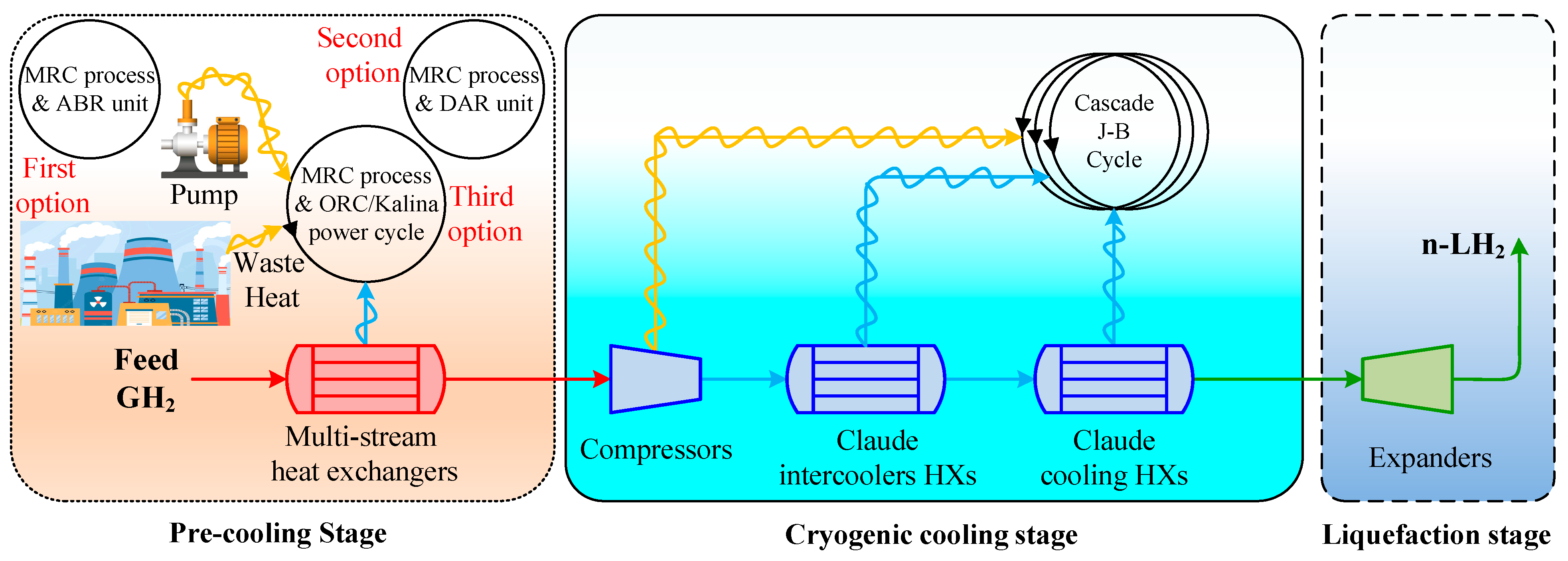
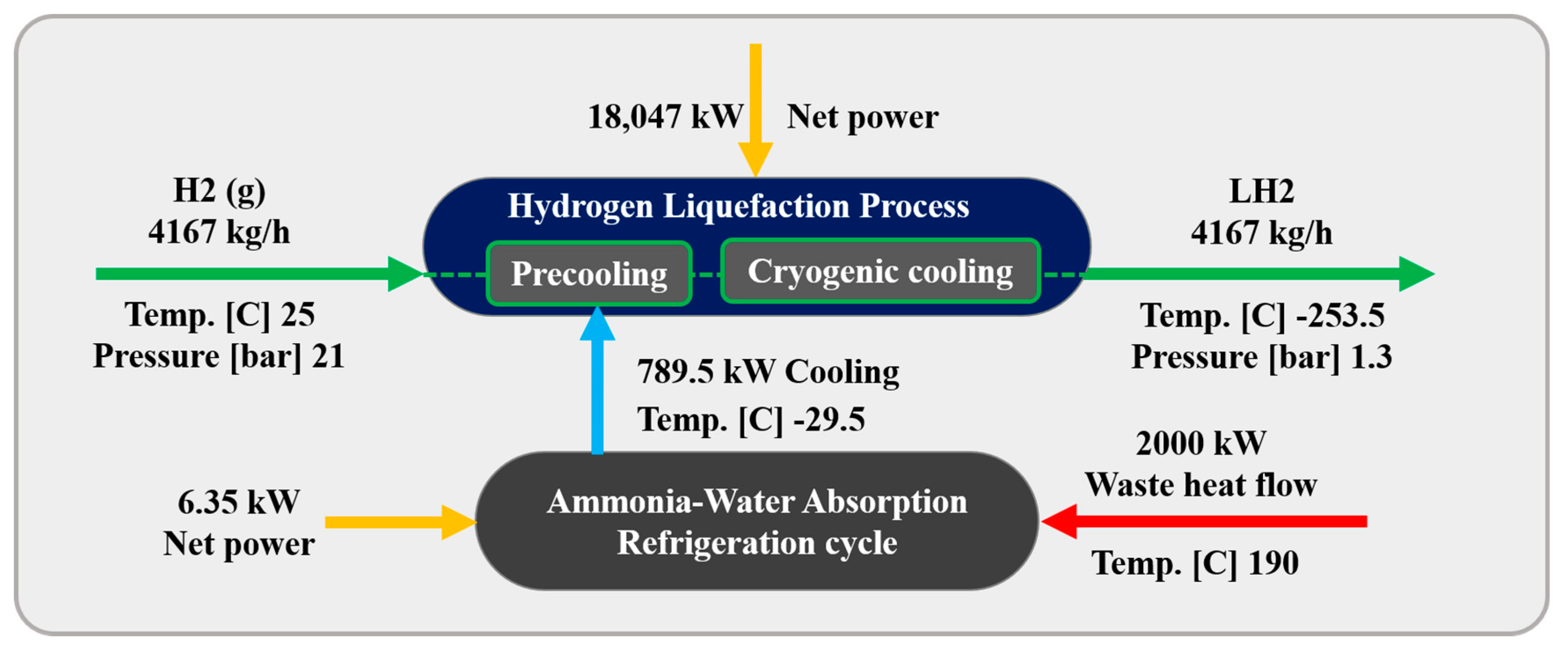


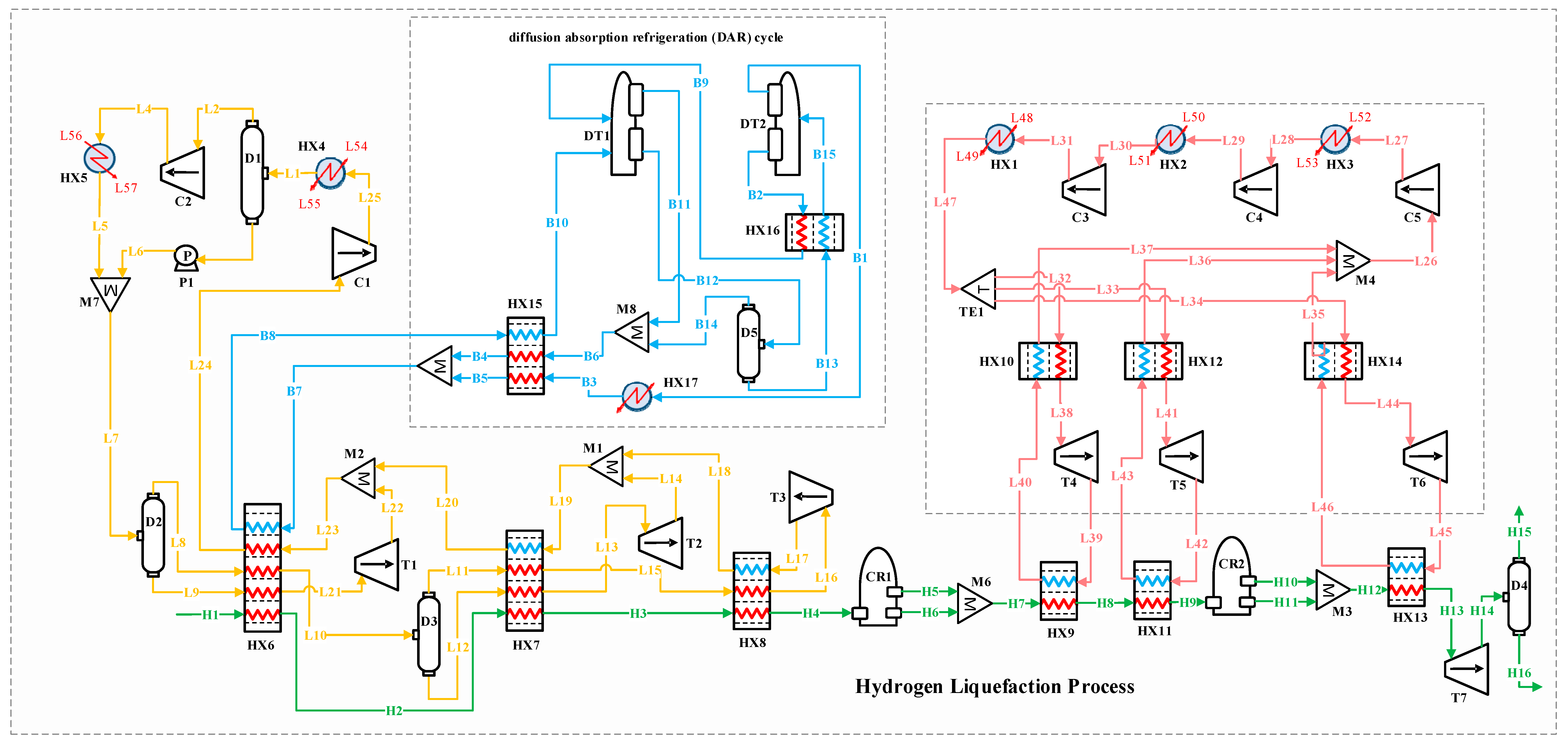
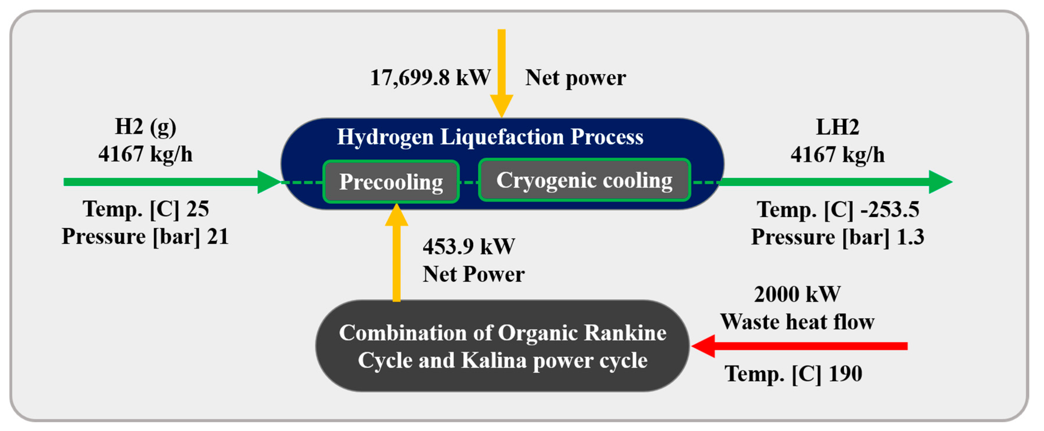

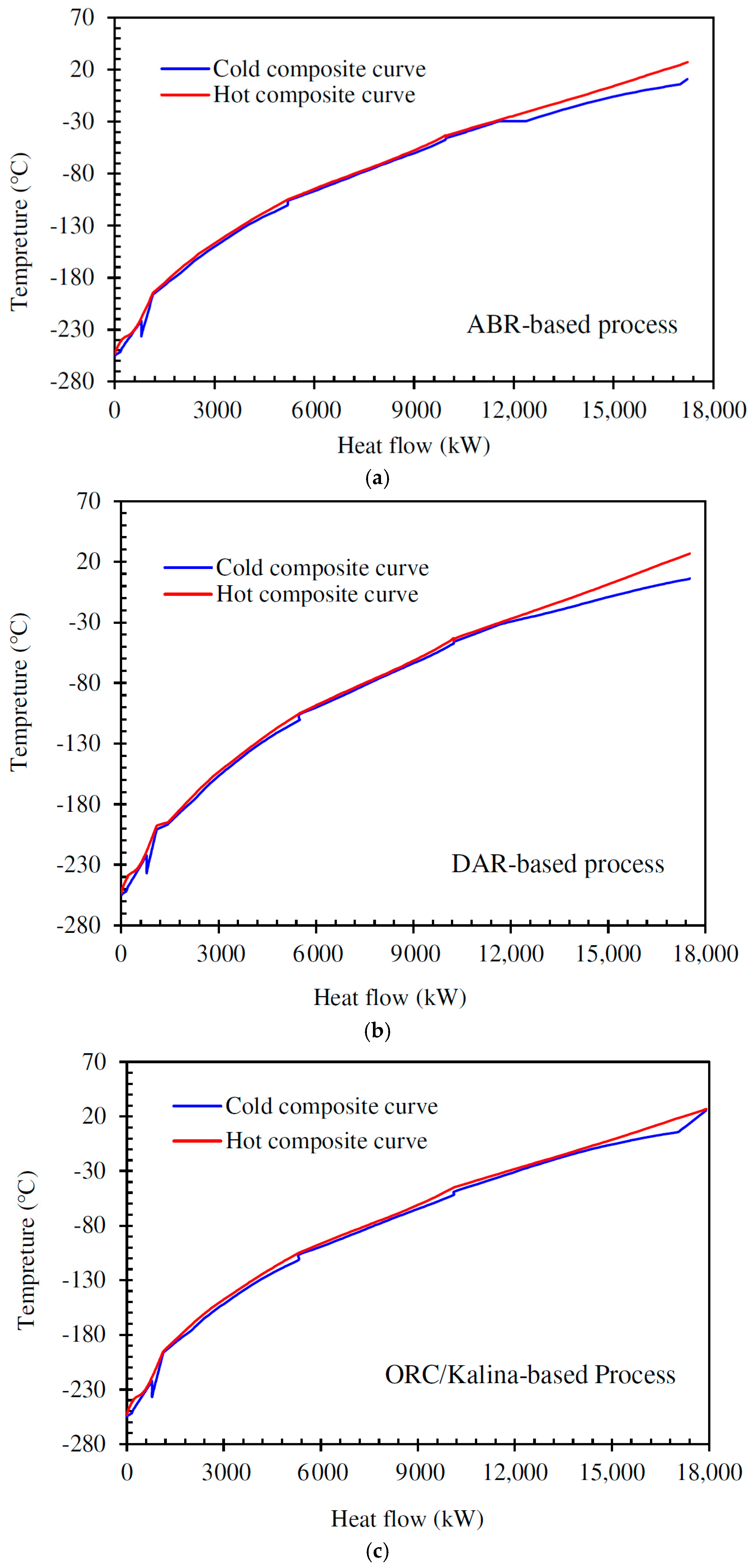
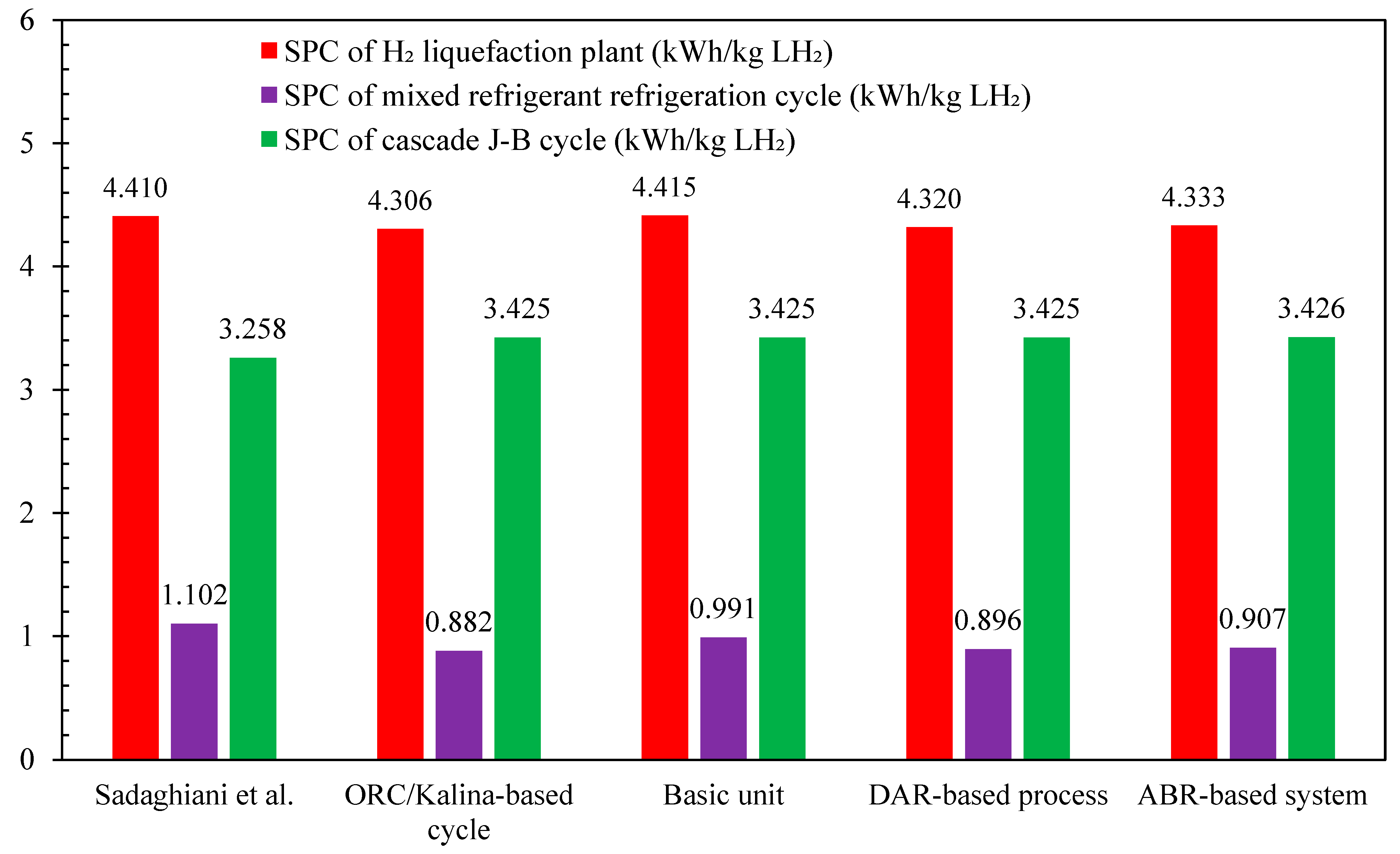
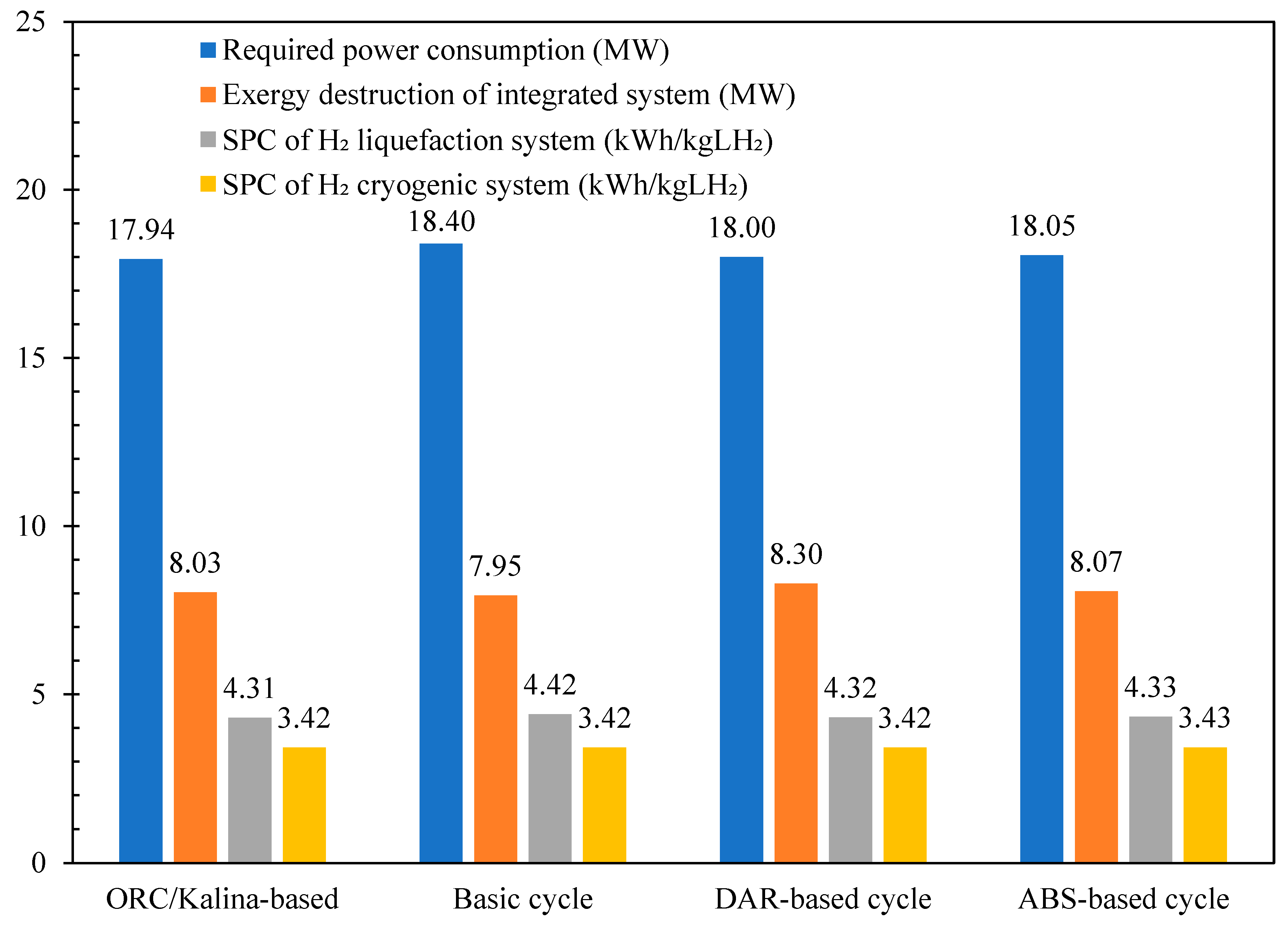
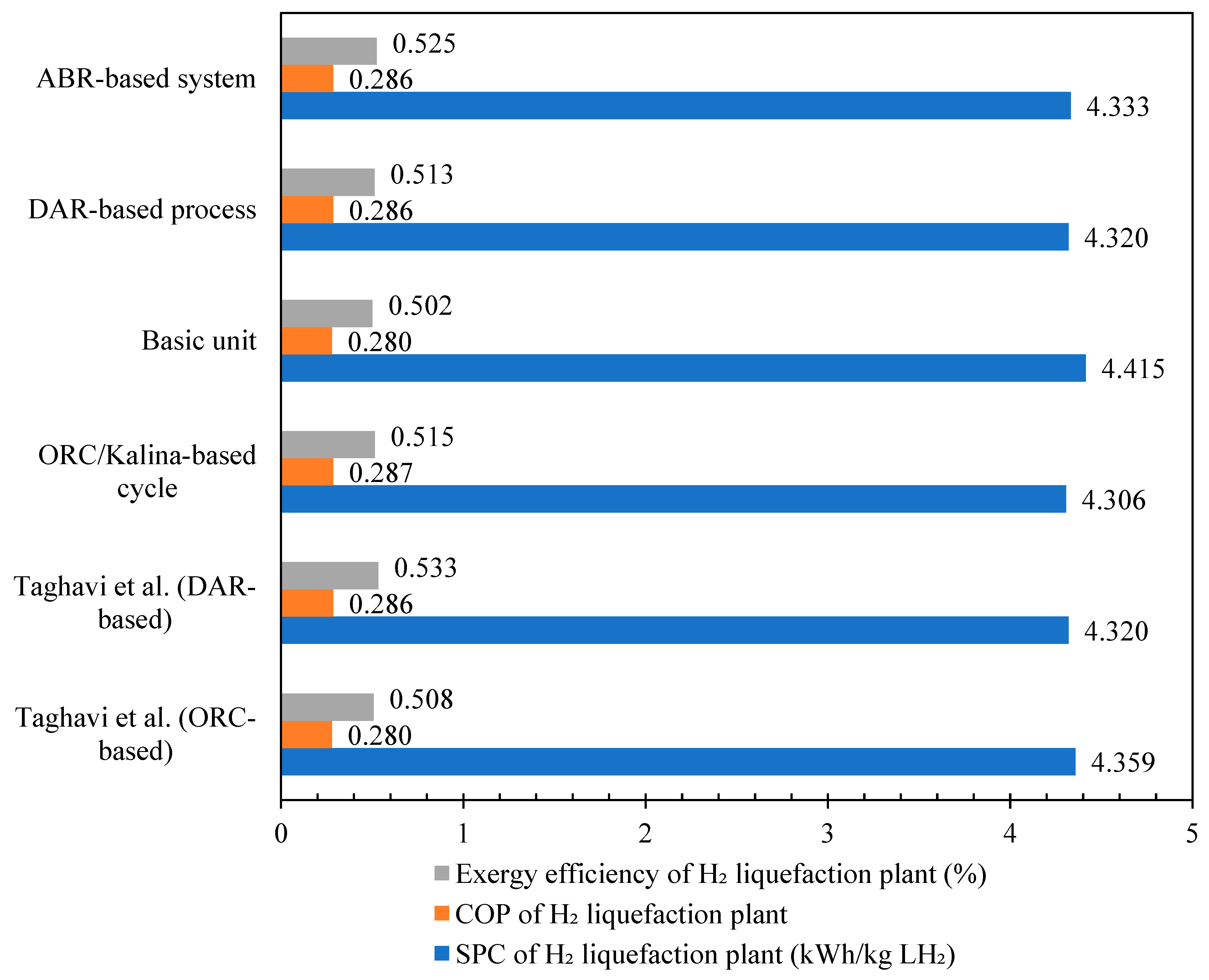
Disclaimer/Publisher’s Note: The statements, opinions and data contained in all publications are solely those of the individual author(s) and contributor(s) and not of MDPI and/or the editor(s). MDPI and/or the editor(s) disclaim responsibility for any injury to people or property resulting from any ideas, methods, instructions or products referred to in the content. |
© 2025 by the authors. Licensee MDPI, Basel, Switzerland. This article is an open access article distributed under the terms and conditions of the Creative Commons Attribution (CC BY) license (https://creativecommons.org/licenses/by/4.0/).