Article

Adaptive Differential Evolution Integration: Algorithm Development and Application to Inverse Heat Conduction

1
School of Automation and Electrical Engineering, Tianjin University of Technology and Education, Tianjin 300222, China
2
Tianjin Key Laboratory of Information Sensing and Intelligent Control, Tianjin 300222, China
*
Authors to whom correspondence should be addressed.
Processes 2025, 13(5), 1293; https://doi.org/10.3390/pr13051293
Submission received: 21 March 2025 / Revised: 19 April 2025 / Accepted: 23 April 2025 / Published: 24 April 2025
(This article belongs to the Special Issue Multi-Phase Flow and Heat and Mass Transfer Engineering)

Abstract

:
In response to the limitations observed in existing single intelligent optimization algorithms, particularly their shortcomings in their global search capability and population diversity, we propose the Adaptive Differential Evolution Integral (ADEI) algorithm. Drawing inspiration from the collective behaviors observed in social organisms, this algorithm introduces four roles—“leaders”, “followers”, “contemplators”, and “rationalists”—employing a dynamic following strategy to effectively integrate these diverse particles and populations. Specifically, individuals in the Differential Evolution algorithm serve as the leader population, with tailored trial vector generation strategies implemented to enhance the global search capability. Concurrently, improvements are made to the particle swarm optimization algorithm to facilitate its role as the evolution strategy for other populations. By adopting this approach, the algorithm’s population diversity is enhanced, striking a balance between the global and local search performance, thereby augmenting its search efficiency and convergence accuracy. Extensive tests using benchmark functions and engineering problems show that the proposed algorithm excels in over half of the 28 test functions. It demonstrates strong convergence and adaptability for unimodal, multimodal, and composite problems. Experiments on solving inverse heat conduction problems validate its effectiveness in real-world scenarios and highlight its potential for engineering applications.

1. Introduction

With the rapid development of computer science and artificial intelligence, intelligent optimization algorithms have become indispensable tools widely deployed in tackling intricate optimization problems such as engineering design [1], resource allocation [2], and production scheduling [3]. These algorithms simulate processes akin to biological evolution and collective behavior in nature to address optimization challenges. Numerous optimization methods have been proposed for a variety of optimization problems, including but not limited to particle swarm optimization (PSO) [4], differential evolution (DE) [5], and genetic algorithm (GAs) [6].
While intelligent optimization algorithms boast robust search capabilities and adaptability, they also encounter challenges such as a low convergence accuracy and susceptibility to local optima. Moreover, selecting the appropriate algorithms and adjusting the parameters judiciously are crucial to attaining the optimal optimization outcomes for different problems. Scholars worldwide have effectively integrated the advantages of various algorithms to enhance the population diversity of the algorithms, as well as their global search capability for different problems. For instance, Zhang et al. [7] proposed a hybrid optimization algorithm combining cuckoo search and DE, employing a multi-population strategy for the global search with cuckoo search and the local search with DE, thus seamlessly integrating the two algorithms. Rosi’c et al. [8] proposed an improved adaptive hybrid firefly differential evolution algorithm which integrated DE operators at different search stages of the firefly algorithm while adaptively adjusting the control parameters to maintain a high population diversity, achieving a balance between global exploration and local exploitation. Khan [9] et al. combined firefly optimization with PSO to devise a hybrid firefly particle swarm algorithm, enhancing the convergence accuracy and acceleration through fusion strategies. The aforementioned scholars have effectively integrated different optimization algorithms, improving the population diversity and enhancing the performance of the algorithms. Furthermore, various improvement strategies have been explored by different researchers for specific basic algorithms to improve the convergence accuracy and convergence speed of these algorithms. For example, Wang et al. [10] proposed a composite differential evolution (CoDE) algorithm, which adopts a more compact mutation crossover representation to reduce the spatial complexity of the search process, and proposed a new trial vector generation method, randomly combining three control parameters to generate the trial vectors, improving the search efficiency and convergence speed of the algorithm. By employing multiple trial vector generation strategies, it expands the search range of the DE algorithm and avoids the limitations caused by a single strategy, thereby enhancing the algorithm’s global search capability [11]. Mohammad et al. [12] proposed a multi-trial vector differential evolution algorithm, constructing three trial vector generators representing particles—a representative particle trial vector generator, a locally random trial vector generator, and a globally historical best trial vector generator—significantly improving the convergence accuracy of the algorithm. Lynn et al. [13] proposed an enhanced particle swarm optimization algorithm (EPSO) which used an adaptive scheme to learn from previously generated dominant individuals in each generation, adaptively determining the best iteration formula for each generation. Sheldon Hui et al. [14] proposed an integrated algorithm based on population arithmetic recombination to solve multimodal optimization problems, which generated new species using adjacent individuals in the local neighborhood to avoid parameterization problems and enhance the local search ability. Tang et al. [15] proposed a multi-strategy adaptive particle swarm optimization algorithm which dynamically controlled the inertia weight of particles based on their diversity and introduced an elite learning strategy to enhance the particle diversity. Meng et al. [16] proposed a hybrid paradigm sorting particle swarm algorithm which adaptively adjusted the ratio and contraction coefficient of each paradigm during iteration and provided a global search solution based on the optimal global historical information, improving the overall performance of the algorithm. In conclusion, designing rational integration strategies to seamlessly blend the strengths of various algorithms and mitigate the shortcomings of basic algorithms is a viable approach to enhancing algorithms’ convergence accuracy.
Despite the progress made by hybrid and improved algorithms, challenges remain in achieving a well-balanced trade-off between global exploration and local exploitation [17]. Many of the existing methods rely on fixed strategies or lack adaptive mechanisms [18], which may limit their effectiveness across diverse problem landscapes. Therefore, there is still a pressing need for an optimization framework that can adaptively integrate the strengths of different algorithms, enhance the search efficiency, and maintain population diversity throughout the evolution process.
To address these challenges, this paper leverages the sociological concept of conformity to introduce the Adaptive Differential Evolution Integration (ADEI) optimization algorithm. By adopting a dynamic tracking strategy and an adaptive multi-trial vector generation strategy, this algorithm optimally utilizes the DE algorithm’s robust global search capability and the PSO algorithm’s rapid convergence speed. The performance of the algorithm has been verified on a benchmark test function and for solving an inverse heat conduction problem.

2. The Adaptive Differential Evolution Integrated Optimization Algorithm Based on a Dynamic Tracking Strategy

2.1. The Basic Idea of the Dynamic Following Integrated Strategy

In sociology, it is believed that individuals’ decision-making is influenced by the behaviors or opinions of others in the group [19], driven by the pursuit of a group consensus, fear of uncertainty [20], or the need for social recognition. When an individual’s acceptance of a particular behavior or opinion reaches or exceeds a certain threshold in their mind, the individual tends to imitate or follow that behavior or opinion, resulting in a conformity effect. This threshold is referred to as the “conformity threshold”, which plays an important role in describing collective behavior and decision-making processes in social groups [21].
Following this idea, we designed a leader population and a mass population to simulate the phenomenon of herd behavior. We assume that a subset of individuals evolves independently, uninfluenced by others, following their own evolutionary rules. These individuals tend to be more dispersed, and as the population approaches stability, they are more likely to generate individuals capable of influencing the trajectory of the entire population. Therefore, we refer to them as the leader population.
For the leader population, we employ an algorithm with strong global search capabilities, enabling it to evolve iteratively according to its designated role. Correspondingly, we design the mass population, where the globally optimal individual is selected from all particles during the evolutionary process. An influence region is then defined around this individual, and the population is subdivided further based on a conformity threshold.
In designing the dynamic following strategy, we draw inspiration from the concept of the conformity threshold. A schematic diagram of the dynamic following strategy is shown in Figure 1.
The circular particles represent the particles of the leading group, with the black particle being the global optimal particle. As illustrated in Figure 1, the update process for the leaders is independent and does not rely on the mass population. The square particles represent the mass group particles, and the numbers inside them indicate their conformity thresholds (decimals between [ 0 ,   1 ] are multiplied by 10 and rounded to facilitate display). Particles with lower conformity thresholds are influenced by the integration effect and become “followers” (blue). Particles with higher thresholds are less susceptible to external influences and become “contemplators” (white). Those with intermediate threshold values become “rationalists” (orange). In each iteration cycle, the global optimal particle and the mass population’s optimal particle are selected. We hypothesize that mass particles within a defined influence radius around the optimal particle, driven by a conformity effect, will exhibit a directed evolutionary movement towards the optimal particle’s position. This influence zone is intentionally restricted to a subset of the population to maintain diversity. Given the superior global exploration capabilities of the leader population, this radius (R) is determined based on the average Euclidean distance between the leader particles and the global optimum, as formulated in Equation (1).
R = d 1 N i = 1 N d = 1 D G b e s t d X i , d 2
where d denotes a scaling factor for the influence radius, D denotes the dimensionality of the search space, N denotes the number of particles in the leading group, X g , d is the position of the global optimal particle in the d-th dimension, and  X i , d is the position of the leading particle i in the d-th dimension. This approach aims to limit the pervasive influence of the optimal particle on the mass population. Specifically, particles within this radius are subject to the conformity effect exerted by the optimal particle. The rationale is that the leader population’s effective global search, resulting in a broader distribution, mitigates the risk of an ill-defined influence radius. Consequently, mass particles outside this radius retain a degree of independence, enhancing global exploration, while those within it experience accelerated convergence due to the pressure of conformity. The Euclidean distance, a simple yet effective measure of the inter-solution proximity in the D-dimensional search space, is employed for this calculation.
Assuming that not all of the instances within this range are follower particles, a portion of the particles exhibits greater independence. Consequently, we randomly assign a conformity threshold to each particle and categorize the follower particles into three groups based on their conformity threshold: “followers” that solely follow the optimal particle within their swarm, “rationalists” capable of observing the global optimal and reflecting on their own experiences, and “contemplators” that observe the swarm optimal and the global optimal and engage in self-reflection. Following this strategy, the mass population is dynamically partitioned during each iteration cycle. As illustrated in the figure, the three mass sub-populations acquire different directions of movement, effectively enhancing the population’s diversity and the search capabilities. The distinct update methods for these different categories of particles will be elaborated upon in subsequent sections.

2.2. The DE-Based Leadership Population

This section introduces the ACDE algorithm employed by the leader population. Due to the characteristics of the leader population, a better global search performance is required. The DE algorithm is adopted as the iterative rule for updating the population. Additionally, the advantages of different mutation operators in terms of the global performance are discussed, and multiple trial vector generation strategies are employed to enhance the basic DE algorithm.
The DE algorithm is a classical intelligent optimization method that maintains a population of candidate solutions. Each individual undergoes mutation, crossover, and selection operations to iteratively refine the solutions based on a fitness function. Given a D-dimensional parameter vector X i , G = [ X i , G 1 , X i , G 2 , , X i , G D ] for the individual i at generation G, the mutation process generates a trial vector v i , G through different strategies. Five common mutation strategies are as follows:
(1) “DE/rand/1”:
v i , G = X r 1 i , G + F X r 2 i , G X r 3 i , G
(2) “DE/best/1”:
v i , G = X b e s t , G + F X r 1 i , G X r 2 i , G
(3) “DE/rand-to-best/1”:
v i , G = X i , G + F X b e s t , G X i , G + F X r 1 i , G X r 2 i , G
(4) “DE/best/2”:
v i , G = X b e s t , G + F X r 1 i , G X r 2 i , G + F X r 3 i , G X r 4 i , G
(5) “DE/rand/2”:
v i , G = X r 1 i , G + F X r 2 i , G X r 3 i , G + F X r 4 i , G X r 5 i , G
where F denotes the scaling factor. The subscripts r 1 i , r 2 i , r 3 i , and r 4 i denote random individual numbers other than individual i among all individuals. X b e s t , G denotes the best individual in the G-th iteration.
After generating the mutation vector according to the above formula, the individual encoding vector X i , G and the mutation vector v i , G undergo a crossover operation to produce the trial vector u i , G = u i , G 1 , u i , G 2 , , u i , G D . For each dimension j of each trial vector, its solution formula is the following:
u i , G j = v i , G j , if rand j ( 0 , 1 ) < C r or j = j rand x i , G j , otherwise
The characteristics of these five trial vector generation strategies can be analyzed using mathematical formulas. The primary distinction between “DE/rand/1” and “DE/best/1” lies in the selection of the base vector. In “DE/rand/1”, the base vector is derived from one individual in the current population, whereas in “DE/best/1”, it stems from the optimal individual in the ongoing iteration round. Clearly, “DE/best/1” continually evolves towards the direction of the optimal individual in each round, resulting in a faster convergence speed. However, as the current optimal and the global optimal may not always align, there is a heightened risk of converging to a local optimum.
“DE/rand-to-best/1”, “DE/best/2”, and “DE/rand/2” all incorporate a difference vector comprising a group of randomly selected individuals, aiming to introduce greater perturbations. “DE/rand/2” exhibits the highest level of randomness, which facilitates the global search. The base vector of “DE/best/2” mirrors the optimal individual in the current iteration round, akin to “DE/rand/1”, thus leading to faster convergence. In “DE/rand-to-best/1”, one term in the difference vector incorporates the disparity between the current optimal individual and the base vector. Consequently, during mutation, it selectively considers the direction of the optimal individual, rendering it a relatively moderate strategy among the three.
To enhance the adaptability, Adaptive Composite Differential Evolution (ACDE) integrates multiple mutation strategies and control parameters dynamically. Inspired by CoDE, ACDE combines different mutation strategies randomly, generating multiple trial vectors per iteration to improve the search efficiency. Additionally, an adaptive stage-wise mechanism selects appropriate strategies at different evolutionary phases. Three additional strategies are introduced:
rand/1/bin:
u i , G = X r 1 i , G + F · X r 2 i , G X r 3 i , G , if rand < C r or j = j r a n d X r 1 i , G otherwise
rand/2/bin:
u i , G = X r 1 i , G + F · X r 2 i , G X r 3 i , G + F · X r 4 i , G X r 5 i , G , if rand < C r or j = j rand X r 1 i , G otherwise
current-to-rand/1 [22]:
u i , G = X i , G + rand · X r 1 i , G X i , G + F · X r 2 i , G X r i i , G
These three trial vector generation strategies are concise expressions of the mutation and crossover operations in the DE algorithm. These strategies enhance the DE algorithm’s flexibility, balancing exploration and exploitation. “rand/1/bin” ensures diverse search directions, “rand/2/bin” introduces additional perturbations for an enhanced global search, and “current-to-rand/1” provides a dynamic balance between the current solutions and randomness, improving the optimization performance. The principle of the ACDE algorithm is shown in Algorithm 1.
In the initial stage of the algorithm, each individual is randomly assigned a trial vector number, thereby obtaining different trial vectors. Fitness values are calculated to obtain the optimal solution. After a certain number of iterations M a x _ i n i t , in each round, the random probability for the current round is calculated based on the known number of individuals assigned to each trial vector strategy. A random number is then used to randomly select the trial vector update formula shown in Equations (8) to (10) to generate new trial vectors and calculate their fitness values. This logic is continuously iterated, updating the optimal solution.

2.3. The PSO-Based Mass Population

Since the trial vector generation formulas used in the aforementioned ACDE tend to have stronger global search capabilities, the ACDE algorithm is used as the leading population. In order to improve the population diversity of the algorithm and its adaptability to solving problems further, the dynamic following strategy is used to integrate the ACDE algorithm and the PSO algorithm. The PSO algorithm is a simple and fast-iterating swarm intelligence optimization algorithm that serves as a mass population. Since the solution vectors in PSO are typically referred to as particles, to avoid confusion, the individuals in the ACDE algorithm are also uniformly referred to as particles. As mentioned in Section 2.1, particles are divided into “followers”, “rationalists”, and “contemplators” according to the conformity threshold.
Algorithm 1: Principle of ACDE algorithm.
Processes 13 01293 i001
The update formula for followers is the following:
v l , d ( t + 1 ) = ω 1 v l , d ( t ) + c 1 r 1 Pbest d ( t ) x l , d ( t ) x l , d ( t + 1 ) = x l , d ( t ) + v l , d ( t + 1 )
The update formula for rationalists is the following:
v l , d ( t + 1 ) = ω 1 v l , d ( t ) + c 1 r 1 Obest l , d ( t ) x l ( t ) + c 2 r 2 Gbest d ( t ) x l , d ( t ) x l , d ( t + 1 ) = x l , d ( t ) + v l , d ( t + 1 )
The update formula for contemplators is the following:
v l , d ( t + 1 ) = ω 1 v l , d ( t ) + c 1 r 1 Obest l , d ( t ) x l , d ( t ) + c 2 r 2 Gbest d ( t ) x l ( t ) + c 3 r 3 Pbest d ( t ) x l , d ( t ) x l , d ( t + 1 ) = x l , d ( t ) + v l , d ( t + 1 )
In these equations, v l , d ( t ) and x l , d ( t ) denote the velocity and position of the l-th particle in the d-th dimension of the search space during the t-th iteration, respectively; O b e s t l , d denotes the historical optimal position of this particle; G b e s t d denotes the position of the globally optimal particle in the d-th dimension; P b e s t d is the position of the optimal particle among the masses in the d-th dimension; r 1 , r 2 , and r 3 are random numbers in [ 0 , 1 ] ; and c 1 , c 2 , and c 3 are the acceleration factors of the PSO algorithm.
When followers update their positions, they are influenced by the conformity effect, tending to mimic the optimal position of the follower population. Consequently, the update formula solely moves from the current position towards the best position (Pbest) of the follower population. Rationals reference their own personal best position ( O b e s t l , d ) and the global best position ( G b e s t d ). Contemplators recognize that neither the global optimal nor the swarm optimal may be the true optimal particle and thus incorporate the directions of both, along with their personal historical best. In other words, the formula includes the reference terms P b e s t d , O b e s t l , d , and G b e s t d ; therefore, during position updates, the velocity vector’s direction combines these three components. We believe that this combination produces three sub-populations with different properties because their search directions are different in most cases, so the search performance will be better. Information exchange is possible between different populations, including the leader population, since G b e s t d can be obtained from the leader population. Simultaneously, during the differential update process, the leader population can utilize the generated G b e s t d from the follower individuals to replace its inferior vectors.
Combining the entire process of the dynamic following strategy and the ACDE algorithm, the operational procedure of the ADEI algorithm is as follows:
1.
Initialize the maximum number of fitness evaluations M a x _ F E S , the dimensionality D of the search space for the optimization problem, the size N of the leader population, the size P of the mass population, the reserve values of the control parameters F and C r for the leading particles, the learning factors c 1 , c 2 , and c 3 for the mass population particles, the inertia weight w 1 , and the influence radius scaling factor d. Randomly initialize the positions of the particles in the leader population within the search space, randomly initialize the positions and velocities of the particles in the mass population, and randomly initialize the conformity thresholds T h r of the mass population particles. To keep track of the number of fitness evaluations, set a counter c o u n t e r = 0 .
2.
Calculate the fitness values of all particles, and during the iterative calculation process, record the optimal particle E b e s t of the leading group and the optimal particle P b e s t of the mass population based on the fitness values. Select the one with smaller fitness as the global optimal particle G b e s t . Update the counter c o u n t e r = N + P .
3.
Calculate the influence radius R of the global optimal particle according to (1). Compute the distances between all crowd particles and the global optimal particle, select all particles within the influence radius, and divide the affected particles into three sub-populations based on their conformity thresholds. Update the velocities and positions of the particles in these sub-populations according to Equations (11) to (13), and calculate the fitness values of the obtained mass population particles to obtain the new optimal particle P b e s t of the mass population. Update the counter c o u n t e r = c o u n t e r + P .
4.
G b e s t is utilized to replace a randomly selected non-optimal solution within the leader population. Generate the trial vectors according to the ACDE in Algorithm 1, calculate the fitness values of all of the trial vectors, update the leader population from the previous generation, and select the optimal particle E b e s t of the leader population. Update the counter c o u n t e r = c o u n t e r + N .
5.
Compare the fitness values of the optimal particle P b e s t of the leader population and the optimal particle E b e s t of the crowd group, and update the global optimal particle G b e s t .
6.
Check whether the maximum number of fitness evaluations has been reached. If c o u n t e r Max _ FES , terminate the optimization and output the vector value of the global optimal particle as the global optimal solution. Otherwise, go to Step 3 and continue the optimization process.

3. Experiments

3.1. Benchmark Function Experiments

The algorithm’s performance is assessed using the CEC2013 [23] suite of classical test functions, comprising 28 functions categorized as follows: 5 unimodal functions ( f 1 f 5 ), 15 multimodal functions ( f 6 f 20 ), and 8 composition functions ( f 21 f 28 ). Notably, the global minima of these functions were deliberately shifted away from the origin. This adjustment aimed to offer a more equitable evaluation criterion, particularly for algorithms capable of rapid convergence to the origin yet exhibiting a subpar optimization performance. To evaluate the performance of the ADEI algorithm, this paper conducted a statistical analysis on the solution results for each test function using the mean and standard deviation from 30 independent repetitions.
(1)
An Ablation Experiment
To isolate the impact of different components of the ADEI algorithm, a comparative analysis was conducted against several variants and baseline algorithms, such as a DE algorithm and CoDE. To evaluate the global search capability of the proposed ADEI algorithm, this paper specifically implements a DE-PSO dynamic following hybrid algorithm with the DE population as the leading population for comparison. This algorithm uses the “DE/rand/1” strategy to generate the trial vectors, with the control parameters set as F = 0.85 and C r = 0.9 . The parameter settings for the DE algorithm are consistent with those for the DE-PSO algorithm; the parameter settings for the CoDE algorithm are consistent with those for the ADEI algorithm. The total number of particles is set to be the same for all algorithms, with 60 particles for DE and CoDE, 30 leading particles, and 30 crowd particles for DE-PSO and ADEI. Each algorithm is employed with a dimensionality of D = 30 , a search range of 100 , 100 D , and a maximum number of function evaluations of Max _ FES = 300,000, adhering to the setup requirements outlined in the CEC2013 test function suite.
We conducted a statistical analysis of the solution results for each test function using the mean and standard deviation from 30 independent repetitions. The detailed data are recorded in Table 1, with the optimal results marked in bold.
From Table 1, it is evident that the ADEI algorithm exhibited a superior average performance across the benchmark functions. Specifically, it achieved the highest average performance on 4 out of 5 unimodal functions, 11 out of 15 multimodal functions, and 5 out of 8 composition functions. The ADEI algorithm exhibits a distinct advantage over both the single DE and CoDE algorithms. The other DE-PSO algorithm employing the dynamic following strategy, except for being slightly worse than DE on f26, outperforms DE on the remaining functions, indicating that the dynamic guidance strategy greatly improves the convergence performance of the DE algorithm. The ADEI algorithm employs an adaptive composite differential strategy and achieves a superior solution quality compared to that with DE-PSO. Although both ADEI and CoDE use multiple trial vector differential strategies, ADEI obtained more optimal solutions, demonstrating its stronger problem adaptability. The experimental data statistics show that the dynamic guidance strategy can effectively balance the global and local search, and algorithms based on this strategy exhibit an excellent convergence accuracy and generalization ability, regardless of unimodal, multimodal, or composition functions.
To evaluate the convergence performance of the ADEI algorithm during the iteration process further, the convergence processes on different types of test functions were plotted. The unimodal functions f 1 , f 3 , and f 5 ; the multimodal functions f 6 , f 11 , and f 12 ; and the composition functions f 22 , f 25 , and f 27 were selected, with their convergence curves shown in Figure 2. In these figures, the horizontal axis represents the number of iterations, and the vertical axis represents the fitness value.
From a comparison of the results of the unimodal test functions f 1 , f 3 , and f 5 in Figure 2, we can see that the convergence accuracy and speed of the ADEI algorithm are superior to those of the other algorithms. In the multimodal function tests, the ADEI algorithm’s convergence accuracy is significantly better than that of the other algorithms on f 6 and f 18 , and it only lags behind the CoDE algorithm on f 12 . Additionally, the ADEI algorithm still exhibits a significant advantage in its convergence speed. The composite function tests show that the ADEI algorithm still converges relatively quickly, reaching convergence within approximately 10 5 fitness evaluations. The ADEI algorithm achieves the significantly highest accuracy on f 22 and consistently demonstrated a relatively high convergence accuracy across the other three convergence graphs. On f 27 , its performance is comparable to that of CoDE. These observations align with the convergence precision results presented in the table.
The results demonstrate that ADEI achieves a superior convergence accuracy and a faster convergence speed in the majority of the function tests. Notably, CoDE exhibits a significant advantage over the original DE in terms of both convergence speed and accuracy. The ACDE algorithm, employed by the leader population in ADEI, integrates principles from the CoDE algorithm. Although ACDE is specifically designed to function as a leader population and is not utilized independently, these findings confirm its effectiveness as a standalone component. Intuitively, single-population algorithms are expected to possess better local search capabilities and potentially faster search speeds, yet the experimental convergence plots reveal contrary outcomes. On most of the test functions, the convergence speed of our designed multi-population algorithms (DE-PSO and ADEI) is significantly faster than that of the single DE or CoDE algorithms. This could be attributed to the diversified candidate solutions within the multi-populations, coupled with well-designed iteration strategies, enabling quicker discovery of global or local optima.
Furthermore, the convergence plots for functions such as f 12 , f 18 , and f 22 demonstrate that ADEI and CoDE exhibit a period of stability followed by a descent, indicating avoidance of local optima constraints. In contrast, the original DE algorithm is prone to local optima entrapment during convergence. This suggests that the multi-trial vector generation strategy effectively enhances the algorithm’s global search capabilities.
(2)
Comparison with State-of-the-Art Algorithms
Several famous or state-of-the-art algorithms, including EPSO [13], MEGWO [24], GEDGWO [25], GWO [26], PSO-sono [16], and FDR-PSO [27], were selected as comparison algorithms. The design of the EPSO algorithm follows the methodology outlined in [13], incorporating a small-scale comprehensive learning PSO (CLPSO) [28] subgroup and a large-scale hybrid subgroup. The latter is an integration of the improved inertia weight PSO [29], gbest-based CLPSO, FDR-PSO, HPSO-TVAC, and LIPS algorithms [30]. The parameter settings for the MEGWO and GEDGWO algorithms were adopted based on the configurations in [31], while the PSO-sono algorithm used the parameter settings described in [16]. All of the algorithms were configured with the same total number of particles. Specifically, the single-population algorithms employed 60 particles, whereas the ADEI algorithm consisted of 30 leader particles and 30 follower particles.
As shown in Table 2 and Table 3, the proposed ADEI algorithm achieves the best average performance on 16 out of 28 functions. In pairwise comparisons with the other state-of-the-art swarm intelligence optimization algorithms—EPSO, MEGWO, GEDGWO, and PSO-sono—ADEI consistently provides more advantageous solutions. The EPSO algorithm, which employs a multi-population strategy, generally outperforms its independent subpopulation counterpart, FDR-PSO, across most problems. Similarly, the MEGWO and GEDGWO algorithms significantly outperform their respective benchmark, GWO.
Despite this, EPSO with the multi-population strategy underperforms relative to ADEI in the experiments presented here, highlighting the effectiveness of the dynamic-following-strategy-based multi-population integration method proposed in this paper. While MEGWO and GEDGWO exhibit stronger problem-solving capabilities for multi-peak and composite problems, they generally perform worse than ADEI on unimodal problems. PSO-sono, which employs a fundamentally different improvement approach from ADEI, outperforms ADEI on 12 problems. Overall, PSO-sono demonstrates strong search capabilities but achieves the optimal solution in only 5 functions, compared to ADEI’s 11. Therefore, across these test functions, ADEI’s adaptability to various problem types is comparable to, if not superior to, that of the current leading intelligent optimization algorithms. The ADEI algorithm excels at balancing global and local search strategies, exhibiting an excellent convergence accuracy and generalization ability across unimodal, multimodal, and composite functions.
The convergence process for unimodal, multimodal, and composite functions is illustrated in Figure 3. As shown, ADEI demonstrates a superior convergence speed and accuracy for the unimodal problems f 1 , f 3 , and f 5 , as well as the multimodal problems f 6 , f 11 , and f 12 . For the composite function problems f 22 , f 25 , and f 27 , while ADEI may not always achieve the highest convergence accuracy, it remains competitive. Overall, ADEI exhibits a performance that is generally superior to that of most algorithms on unimodal and multimodal functions. Based on the results presented in Table 2 and Table 3, and Figure 3, ADEI demonstrates a superior performance across most optimization problems and exhibits competitive advantages when compared to other state-of-the-art algorithms.

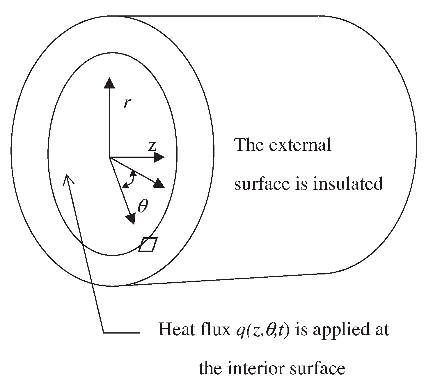
3.2. Three-Dimensional Inverse Heat Conduction Problem Experiments

This experiment aims to validate the performance of the ADEI algorithm in estimating the heat flux distribution on an inner surface by solving a three-dimensional inverse heat conduction problem [32]. The problem originates from the field of heat conduction in engineering and holds practical application and research value.
Consider a cylindrical channel, as shown in Figure 4, where the inner surface ( r = r i ) is subjected to an unknown heat flux q ( z ,   θ ,   t ) , while the outer surface ( r = r o ) is insulated. The thermal properties of the material, such as its thermal conductivity k, density ρ , and specific heat capacity C p , as well as the initial temperature T, are known. Temperature sensors are placed on the outer surface to measure the temperature Y ( r o ,   θ ,   z ,   t ) . The optimization algorithm is employed to estimate the heat flux distribution q ( z ,   θ ,   t ) on the inner surface such that the difference between the computed temperature T ( r o ,   θ ,   z ,   t ) and the measured value Y ( r o ,   θ ,   z ,   t ) is minimized.
The governing equation for this heat conduction problem is [33]
ρ C p T t = k 2 T r 2 + 1 r T r + 1 r 2 2 T θ 2 + 2 T z 2
with the boundary conditions such that at r = r o , k T r = 0 (insulation); at r = r i , k T r = q ( θ ,   z ,   t ) ; and at z = 0 and z = L , k T z = 0 ; the initial conditions are given by T ( r ,   θ ,   z ,   0 ) = T .
The objective function is defined as the sum of the squared residuals between the measured temperature and the computed temperature [32]:
f ( q ( θ ,   z ,   t ) ) = 0 t 0 L 0 2 π [ T ( r o ,   θ ,   z ,   t ) Y ( r o ,   θ ,   z ,   t ) ] 2 d θ d z d t
The optimization algorithm seeks the heat flux distribution q ( θ ,   z ,   t ) that minimizes this objective function. The decision variables represent the spatial and temporal distribution of the inner surface heat flux q ( z ,   θ ,   t ) , whose feasible range is determined based on practical engineering considerations, subject to the constraints that the heat flux must be non-negative and physically realizable.
For the experimental setup, the computational domain is discretized into 10, 40, and 60 grid points in the r, θ , and z directions, respectively. The measurement time interval is set to 0.01 s, with a total measurement duration of 0.45 s, resulting in 45 time steps. The reference temperature data are obtained by solving the forward problem, serving as the “true” temperature distribution in the simulation. The optimization is performed using a population size of M = 50 and a maximum iteration count of 2000 generations.
Using these settings, the ADEI algorithm is applied to the inverse heat conduction problem, and its estimation accuracy, convergence speed, and stability are evaluated under different noise levels. The performance of ADEI is compared with that of other algorithms to demonstrate its effectiveness and superiority.
Two forms of heat flux functions are considered to simulate different heat flux variations. The first form is a step function given by
q ( z ,   θ ,   t ) = q max · 2 z 2 L 2 + 2 z L + 0.5 · ( 0.7 0.3 cos ( θ ) ) , 0.1 t 0.35 0 , otherwise
where q max represents the maximum heat flux set to 100 kW/m²; L denotes the length of the cylindrical channel set to 0.3 m, while z and θ represent the axial and angular coordinates, respectively; and t represents time. This heat flux function exhibits a spatially distributed stepwise variation within the time interval [ 0.1 , 0.35 ] s while remaining zero at other times.
The second form is a ramp variation in which the heat flux increases linearly from zero at t = 0.1 s to its maximum value at t = 0.225 s and then decreases linearly back to zero at t = 0.35 s, simulating a gradual heat flux transition. The physical model parameters used in this study are summarized in Table 4.
These parameters are derived from the waste heat flux problem in helicon plasma discharge within rocket applications, where the material considered is a quartz tube. They define the fundamental physical characteristics of the heat conduction problem and serve as the foundation for numerical simulations and optimization algorithm validation.
Figure 5 presents the estimation results for the step heat flux at positions A (0.15, 0°), B (0.1, 45°), and C (0.04, 90°) using the ADEI algorithm. In the notation ( · ,   · ) , the first value represents z, and the second value represents θ . As shown in Figure 5, the heat flux at three different positions exhibits the expected step or ramp form. The surface heat flux obtained by the ADEI algorithm is very close to the known surface heat flux, indicating its good performance in solving surface heat flux problems. Since this method has no special requirements for the objective function, it is more advantageous than gradient-based methods in solving step or ramp heat flux problems that are not differentiable everywhere. The results demonstrate the feasibility of the program and the ability of the ADEI algorithm to recover the inner surface heat flux without any prior information on the unknown transient functions.
Table 5 records the maximum absolute error (MaxAE), root mean square error (RMSE), and mean absolute error (MAE) between the estimated step heat flux and the exact results at these three different positions. It can be seen that the ADEI algorithm has the smallest error among those of all of the compared algorithms. This further demonstrates the superior performance of the ADEI algorithm in inverse surface heat flux calculations.

4. Conclusions

This paper proposes the Adaptive Differential Evolution Integration (ADEI) optimization algorithm, which incorporates an adaptive composite differential evolution strategy and a dynamic follow-up strategy. The algorithm is designed to enhance the convergence accuracy, maintain population diversity, and avoid local optima. The main contributions of this work are as follows:
(1) An adaptive trial vector generation strategy is developed based on the composite CoDE framework. This strategy addresses the limitations of traditional DE by improving both the convergence accuracy and convergence speed through diversified vector generation and parameter adaptation. (2) A dynamic follow-up strategy is introduced to seamlessly integrate the adaptive CoDE with the particle swarm optimization (PSO) algorithm. This mechanism enhances the population diversity and strengthens the global search capabilities, reducing the risk of premature convergence. (3) By combining the above two strategies, a novel hybrid algorithm, ADEI, is proposed, achieving a synergistic balance between global exploration and local exploitation.
To validate the effectiveness of the proposed algorithm, extensive experiments were conducted on 28 benchmark functions from the CEC2013 test suite, as well as an inverse heat conduction problem. The key findings are summarized as follows:
(1) Compared with traditional DE, the adaptive composite strategy significantly improves the convergence accuracy and search efficiency, particularly on high-dimensional and multimodal functions. (2) The algorithms enhanced with the dynamic follow-up strategy (DE-PSO and ADEI) consistently outperform their base variants (DE and PSO), demonstrating that this strategy effectively mitigates the tendency to fall into local optima. (3) The proposed ADEI algorithm exhibits strong adaptability across a wide range of optimization problems. Furthermore, its successful application to the inverse heat conduction problem highlights its practical value and potential for solving complex engineering problems.
In future work, we plan to explore the integration of problem-specific knowledge and adaptive parameter control mechanisms to improve the performance and robustness of the ADEI algorithm in real-world scenarios further.

Author Contributions

Conceptualization, Z.Z.; Methodology, Z.L.; Software, H.L. and Y.S.; Validation, Z.L.; Formal analysis, Z.L.; Resources, H.L. and Y.S.; Data curation, Z.L.; Writing—original draft, H.L. and Y.S.; Supervision, Z.Z.; Project administration, Z.Z. All authors have read and agreed to the published version of the manuscript.

Funding

This work was supported by Natural Science Foundation of Tianjin (No. 22JCQNJC01100) and the PhD Research Start-up Fund of Tianjin Univ Technol & Educ (grant number KRKC012356).

Data Availability Statement

The original contributions presented in this study are included in the article. Further inquiries can be directed to the corresponding authors.

Conflicts of Interest

The authors declare no conflicts of interest.

References

  1. Shen, Y.; Zhang, C.; Gharehchopogh, F.S.; Mirjalili, S. An improved whale optimization algorithm based on multi-population evolution for global optimization and engineering design problems. Expert Syst. Appl. 2023, 215, 119269. [Google Scholar] [CrossRef]
  2. Teekaraman, Y.; Manoharan, H.; Basha, A.R.; Manoharan, A. Hybrid optimization algorithms for resource allocation in heterogeneous cognitive radio networks. Neural Process. Lett. 2023, 55, 3813–3826. [Google Scholar] [CrossRef]
  3. Wang, L.; Zhao, Y.; Yin, X. Precast production scheduling in off-site construction: Mainstream contents and optimization perspective. J. Clean. Prod. 2023, 405, 137054. [Google Scholar] [CrossRef]
  4. Jain, M.; Saihjpal, V.; Singh, N.; Singh, S.B. An overview of variants and advancements of PSO algorithm. Appl. Sci. 2022, 12, 8392. [Google Scholar] [CrossRef]
  5. Ahmad, M.F.; Isa, N.A.M.; Lim, W.H.; Ang, K.M. Differential evolution: A recent review based on state-of-the-art works. Alex. Eng. J. 2022, 61, 3831–3872. [Google Scholar] [CrossRef]
  6. Papazoglou, G.; Biskas, P. Review and comparison of genetic algorithm and particle swarm optimization in the optimal power flow problem. Energies 2023, 16, 1152. [Google Scholar] [CrossRef]
  7. Zhang, Z.; Ding, S.; Jia, W. A hybrid optimization algorithm based on cuckoo search and differential evolution for solving constrained engineering problems. Eng. Appl. Artif. Intell. 2019, 85, 254–268. [Google Scholar] [CrossRef]
  8. Rosić, M.B.; Simić, M.I.; Pejović, P.V. An improved adaptive hybrid firefly differential evolution algorithm for passive target localization. Soft Comput. 2021, 25, 5559–5585. [Google Scholar] [CrossRef]
  9. Khan, A.; Hizam, H.; bin Abdul Wahab, N.I.; Lutfi Othman, M. Optimal power flow using hybrid firefly and particle swarm optimization algorithm. PLoS ONE 2020, 15, e0235668. [Google Scholar] [CrossRef]
  10. Wang, Y.; Cai, Z.; Zhang, Q. Differential evolution with composite trial vector generation strategies and control parameters. IEEE Trans. Evol. Comput. 2011, 15, 55–66. [Google Scholar] [CrossRef]
  11. Eltaeib, T.; Dichter, J. Data optimization with differential evolution strategies: A survey of the state-of-the-art. In Proceedings of the 2017 IEEE International Conference on Power, Control, Signals and Instrumentation Engineering (ICPCSI), Chennai, India, 21–22 September 2017; pp. 17–23. [Google Scholar]
  12. Nadimi-Shahraki, M.H.; Taghian, S.; Mirjalili, S.; Faris, H. MTDE: An effective multi-trial vector-based differential evolution algorithm and its applications for engineering design problems. Appl. Soft Comput. 2020, 97, 106761. [Google Scholar] [CrossRef]
  13. Lynn, N.; Suganthan, P.N. Ensemble particle swarm optimizer. Appl. Soft Comput. 2017, 55, 533–548. [Google Scholar] [CrossRef]
  14. Hui, S.; Suganthan, P.N. Ensemble and arithmetic recombination-based speciation differential evolution for multimodal optimization. IEEE Trans. Cybern. 2015, 46, 64–74. [Google Scholar] [CrossRef] [PubMed]
  15. Tang, K.; Li, Z.; Luo, L.; Liu, B. Multi-strategy adaptive particle swarm optimization for numerical optimization. Eng. Appl. Artif. Intell. 2015, 37, 9–19. [Google Scholar] [CrossRef]
  16. Meng, Z.; Zhong, Y.; Mao, G.; Liang, Y. PSOsono: A novel PSO variant for single-objective numerical optimization. Inf. Sci. 2022, 586, 176–191. [Google Scholar] [CrossRef]
  17. El-Mihoub, T.A.; Hopgood, A.A.; Nolle, L.; Battersby, A. Hybrid Genetic Algorithms: A Review. Eng. Lett. 2006, 13, 124–137. [Google Scholar]
  18. Hu, G.; Zhong, J.; Du, B.; Wei, G. An enhanced hybrid arithmetic optimization algorithm for engineering applications. Comput. Methods Appl. Mech. Eng. 2022, 394, 114901. [Google Scholar] [CrossRef]
  19. Spears, R. Social influence and group identity. Annu. Rev. Psychol. 2021, 72, 367–390. [Google Scholar] [CrossRef]
  20. Melamed, D.; Savage, S.V.; Munn, C. Uncertainty and social influence. Socius 2019, 5, 2378023119866971. [Google Scholar] [CrossRef]
  21. Liu, X.; Huang, C.; Dai, Q.; Yang, J. The effects of the conformity threshold on cooperation in spatial prisoner’s dilemma games. Europhys. Lett. 2019, 128, 18001. [Google Scholar] [CrossRef]
  22. Zhou, T.; Hu, Z.; Su, Q.; Xiong, W. A clustering differential evolution algorithm with neighborhood-based dual mutation operator for multimodal multiobjective optimization. Expert Syst. Appl. 2023, 216, 119438. [Google Scholar] [CrossRef]
  23. Liang, J.J.; Qu, B.; Suganthan, P.N.; Hernández-Díaz, A.G. Problem Definitions and Evaluation Criteria for the CEC 2013 Special Session on Real-Parameter Optimization; Technical Report; Computational Intelligence Laboratory, Zhengzhou University: Zhengzhou, China; Nanyang Technological University: Singapore, 2013; Volume 201212, pp. 281–295. [Google Scholar]
  24. Wang, X.; Zhao, H.; Han, T.; Zhou, H.; Li, C. A grey wolf optimizer using Gaussian estimation of distribution and its application in the multi-UAV multi-target urban tracking problem. Appl. Soft Comput. 2019, 78, 240–260. [Google Scholar] [CrossRef]
  25. Tu, Q.; Chen, X.; Liu, X. Multi-strategy ensemble grey wolf optimizer and its application to feature selection. Appl. Soft Comput. 2019, 76, 16–30. [Google Scholar] [CrossRef]
  26. Mirjalili, S.; Mirjalili, S.M.; Lewis, A. Grey wolf optimizer. Adv. Eng. Softw. 2014, 69, 46–61. [Google Scholar] [CrossRef]
  27. Cleghorn, C.W.; Engelbrecht, A.P. Fitness-distance-ratio particle swarm optimization: Stability analysis. In Proceedings of the Genetic and Evolutionary Computation Conference, Berlin, Germany, 15–19 July 2017; pp. 12–18. [Google Scholar]
  28. Liang, J.J.; Qin, A.K.; Suganthan, P.N.; Baskar, S. Comprehensive learning particle swarm optimizer for global optimization of multimodal functions. IEEE Trans. Evol. Comput. 2006, 10, 281–295. [Google Scholar] [CrossRef]
  29. Shi, Y.; Eberhart, R.C. Empirical study of particle swarm optimization. In Proceedings of the 1999 congress on evolutionary computation-CEC99 (Cat. No. 99TH8406), Washington, DC, USA, 6–9 July 1999; Volume 3, pp. 1945–1950. [Google Scholar]
  30. Qu, B.Y.; Suganthan, P.N.; Das, S. A distance-based locally informed particle swarm model for multimodal optimization. IEEE Trans. Evol. Comput. 2012, 17, 387–402. [Google Scholar] [CrossRef]
  31. Zhang, X.; Lin, Q.; Mao, W.; Liu, S.; Dou, Z.; Liu, G. Hybrid Particle Swarm and Grey Wolf Optimizer and its application to clustering optimization. Appl. Soft Comput. 2021, 101, 107061. [Google Scholar] [CrossRef]
  32. Liu, F.B. Particle swarm optimization-based algorithms for solving inverse heat conduction problems of estimating surface heat flux. Int. J. Heat Mass Transf. 2012, 55, 2062–2068. [Google Scholar] [CrossRef]
  33. Udayraj; Mulani, K.; Talukdar, P.; Das, A.; Alagirusamy, R. Performance analysis and feasibility study of ant colony optimization, particle swarm optimization and cuckoo search algorithms for inverse heat transfer problems. Int. J. Heat Mass Transf. 2015, 89, 359–378. [Google Scholar]
Figure 1. A schematic diagram of the proposed dynamic tracking strategy.
Processes 13 01293 g001
Figure 2. Convergence processes of different test functions compared with the ADEI algorithm.
Processes 13 01293 g002
Figure 3. A comparison of convergence curves for the state-of-the-art algorithms. (ai) show the convergence process of the seven algorithms on f 1 , f 3 , f 5 , f 6 , f 11 , f 12 , f 22 , f 25 , and f 27 , respectively.
Processes 13 01293 g003
Figure 4. A physical model of the three-dimensional inverse heat conduction problem.
Processes 13 01293 g004
Figure 5. Inverse solutions of heat fluxes using the ADEI algorithm at locations A, B, and C.
Processes 13 01293 g005
Table 1. A comparison of the results of the ablation experiment.
DECoDEDE-PSOADEI
f11.15 × 10 1  ± 6.68 × 10 2 0 . 00 × 10 0  ±  0 . 00 × 10 0 1.14 × 10 13  ± 1.14 × 10 13 0 . 00 × 10 0  ±  0 . 00 × 10 0
f22.02 × 10 7  ± 8.01 × 10 6 2.96 × 10 5  ± 1.74 × 10 5 5.14 × 10 5  ± 1.72 × 10 5 5 . 14 × 10 4  ±  1 . 47 × 10 4
f34.29 × 10 8  ± 2.05 × 10 8 2 . 16 × 10 3  ±  2 . 75 × 10 3 1.12 × 10 6  ± 2.17 × 10 6 1.84 × 10 6  ± 2.87 × 10 6
f43.95 × 10 4  ± 6.68 × 10 3 3.91 × 10 1  ± 5.08 × 10 1 3.12 × 10 3  ± 1.47 × 10 3 8 . 44 × 10 2  ±  1 . 31 × 10 1
f52.34 × 10 1  ± 6.91 × 10 2 1 . 14 × 10 13  ±  0 . 00 × 10 0 1.36 × 10 13  ± 4.55 × 10 14 1 . 14 × 10 13  ±  0 . 00 × 10 0
f61.79 × 10 1  ± 1.27 × 10 0 5.61 × 10 0  ± 6.89 × 10 1 1.21 × 10 1  ± 7.17 × 10 0 3 . 35 × 10 1  ±  6 . 19 × 10 1
f75.61 × 10 1  ± 9.13 × 10 0 9.56 × 10 0  ± 6.23 × 10 0 6.23 × 10 0  ± 5.19 × 10 0 9 . 54 × 10 0  ±  5 . 42 × 10 0
f82.10 × 10 1  ± 2.81 × 10 2 2.09 × 10 1  ± 4.62 × 10 2 2.10 × 10 1  ± 4.31 × 10 2 2 . 08 × 10 1  ±  1 . 08 × 10 1
f93.97 × 10 1  ± 7.46 × 10 1 1 . 17 × 10 1  ±  3 . 57 × 10 0 2.38 × 10 1  ± 9.17 × 10 0 1.32 × 10 1  ± 3.27 × 10 0
f105.31 × 10 0  ± 1.66 × 10 0 1.48 × 10 2  ± 1.10 × 10 2 1 . 23 × 10 2  ±  9 . 67 × 10 3 3.19 × 10 2  ± 2.22 × 10 2
f111.40 × 10 2  ± 3.99 × 10 1 4.54 × 10 2  ± 6.27 × 10 2 2.78 × 10 1  ± 5.43 × 10 0 5 . 68 × 10 15  ±  1 . 71 × 10 14
f122.44 × 10 2  ± 1.02 × 10 1 2 . 85 × 10 1  ±  1 . 14 × 10 1 1.58 × 10 2  ± 7.07 × 10 1 3.62 × 10 1  ± 1.06 × 10 1
f132.42 × 10 2  ± 1.79 × 10 1 6 . 28 × 10 1  ±  2 . 01 × 10 1 2.09 × 10 2  ± 1.06 × 10 1 8.33 × 10 1  ± 2.85 × 10 1
f144.98 × 10 3  ± 9.12 × 10 2 5.68 × 10 2  ± 9.21 × 10 1 1.11 × 10 3  ± 2.39 × 10 2 1 . 49 × 10 0  ±  1 . 62 × 10 0
f157.50 × 10 3  ± 2.53 × 10 2 5.96 × 10 3  ± 1.02 × 10 3 7.39 × 10 3  ± 3.22 × 10 2 3 . 25 × 10 3  ±  3 . 91 × 10 2
f161.03 × 10 2  ± 3.18 × 10 1 1.02 × 10 2  ± 3.24 × 10 1 1.02 × 10 2  ± 2.93 × 10 1 1 . 00 × 10 2  ±  2 . 17 × 10 1
f172.65 × 10 2  ± 2.28 × 10 1 1.42 × 10 2  ± 1.24 × 10 0 1.70 × 10 2  ± 9.08 × 10 0 1 . 30 × 10 2  ±  4 . 78 × 10 3
f183.73 × 10 2  ± 1.02 × 10 1 3.02 × 10 2  ± 7.46 × 10 0 3.31 × 10 2  ± 1.79 × 10 1 1 . 60 × 10 2  ±  1 . 34 × 10 1
f191.19 × 10 2  ± 1.84 × 10 0 1.07 × 10 2  ± 3.07 × 10 1 1.03 × 10 2  ± 8.46 × 10 1 1 . 02 × 10 2  ±  3 . 93 × 10 1
f201.13 × 10 2  ± 2.67 × 10 1 1.12 × 10 2  ± 1.60 × 10 1 1.13 × 10 2  ± 1.72 × 10 1 1 . 11 × 10 2  ±  5 . 01 × 10 1
f213.88 × 10 2  ± 4.07 × 10 1 4.37 × 10 2  ± 9.40 × 10 1 3 . 84 × 10 2  ±  6 . 94 × 10 1 4.47 × 10 2  ± 8.36 × 10 1
f224.76 × 10 3  ± 1.51 × 10 3 1.51 × 10 3  ± 2.39 × 10 2 1.13 × 10 3  ± 3.05 × 10 2 2 . 16 × 10 2  ±  5 . 11 × 10 0
f237.46 × 10 3  ± 1.92 × 10 2 6.63 × 10 3  ± 6.19 × 10 2 7.33 × 10 3  ± 3.25 × 10 2 3 . 44 × 10 3  ±  5 . 89 × 10 2
f243.66 × 10 2  ± 1.17 × 10 1 3 . 06 × 10 2  ±  2 . 89 × 10 0 3.31 × 10 2  ± 6.65 × 10 0 3.23 × 10 2  ± 9.64 × 10 0
f253.66 × 10 2  ± 7.98 × 10 0 3 . 48 × 10 2  ±  5 . 82 × 10 0 3.50 × 10 2  ± 5.07 × 10 0 3.53 × 10 2  ± 7.71 × 10 0
f263.02 × 10 2  ± 6.61 × 10 1 3 . 00 × 10 2  ±  6 . 66 × 10 3 3.26 × 10 2  ± 5.26 × 10 1 3.12 × 10 2  ± 3.62 × 10 1
f271.32 × 10 3  ± 1.27 × 10 2 5 . 72 × 10 2  ±  7 . 46 × 10 1 6.58 × 10 2  ± 6.21 × 10 1 6.65 × 10 2  ± 1.20 × 10 2
f284.16 × 10 2  ± 6.22 × 10 0 4.00 × 10 2  ± 2.93 × 10 9 4.00 × 10 2  ± 2.91 × 10 9 4 . 00 × 10 2  ±  1 . 37 × 10 13
+/−/=1/27/010/17/14/24/0-/-/-
Note: The last row of “+/−/=” records the cases where the ADEI algorithm performed better, worse, or equal compared to the other algorithms. The best result achieved for each test function is highlighted in bold for clarity.
Table 2. Comparison of results with famous algorithms.
FDR-PSO GWO EPSO ADEI
MeanStd.RankMeanStd.RankMeanStd.RankMeanStd.Rank
f19.69  × 10 1 2.92  × 10 1 7 8.47  × 10 2 7.47  × 10 2 7 2.04  × 10 13 6.62  × 10 14 3 0.00  × 10 0 0.00  × 10 0 1
f21.87  × 10 7 5.96  × 10 6 7 2.07  × 10 7 1.00  × 10 7 7 2.61  × 10 6 7.82  × 10 5 4 5.14  × 10 4 1.47  × 10 4 1
f34.76  × 10 8 3.18  × 10 8 7 2.71  × 10 9 2.56  × 10 9 7 9.79  × 10 7 1.34  × 10 8 4 1.84  × 10 6 2.87  × 10 6 1
f43.90  × 10 3 6.12  × 10 2 6 2.90  × 10 4 7.59  × 10 3 7 6.01  × 10 3 2.12  × 10 3 6 8.44  × 10 2 1.31  × 10 1 1
f52.07  × 10 1 7.54  × 10 0 7 6.69  × 10 2 3.83  × 10 2 7 2.05  × 10 13 6.83  × 10 14 3 1.14  × 10 13 0.00  × 10 0 2
f65.08  × 10 1 2.46  × 10 1 6 1.18  × 10 2 2.50  × 10 1 7 1.89  × 10 1 1.61  × 10 1 3 3.35  × 10 1 6.19  × 10 1 1
f73.38  × 10 1 9.60  × 10 0 6 4.14  × 10 1 1.43  × 10 1 7 1.68  × 10 1 3.83  × 10 0 2 9.54  × 10 0 5.42  × 10 0 1
f82.09  × 10 1 6.81  × 10 2 3 2.09  × 10 1 5.79  × 10 2 6 2.09  × 10 1 4.54  × 10 2 2 2.08  × 10 1 1.08  × 10 1 1
f92.20  × 10 1 3.62  × 10 0 7 1.84  × 10 1 2.48  × 10 0 3 1.61  × 10 1 2.52  × 10 0 2 1.32  × 10 1 3.27  × 10 0 1
f103.02  × 10 1 1.11  × 10 1 7 2.25  × 10 2 1.29  × 10 2 7 9.17  × 10 2 7.62  × 10 2 4 3.19  × 10 2 2.22  × 10 2 1
f118.38  × 10 1 1.84  × 10 1 7 8.78  × 10 1 3.20  × 10 1 7 1.39  × 10 1 7.67  × 10 0 3 5.68  × 10 15 1.71  × 10 14 1
f121.73  × 10 2 1.31  × 10 1 8 1.23  × 10 2 5.78  × 10 1 5 1.47  × 10 2 4.13  × 10 1 6 3.62  × 10 1 1.06  × 10 1 2
f131.78  × 10 2 2.26  × 10 1 7 1.65  × 10 2 4.21  × 10 1 5 1.83  × 10 2 1.07  × 10 1 7 8.33  × 10 1 2.85  × 10 1 1
f142.61  × 10 3 4.40  × 10 2 6 2.74  × 10 3 4.98  × 10 2 7 4.94  × 10 2 3.73  × 10 2 3 1.49  × 10 0 1.62  × 10 0 1
f156.07  × 10 3 5.32  × 10 2 7 3.41  × 10 3 1.26  × 10 3 2 6.56  × 10 3 3.96  × 10 2 7 3.25  × 10 3 3.91  × 10 2 1
f161.02  × 10 2 4.18  × 10 1 7 2.46  × 10 0 3.01  × 10 1 4 1.03  × 10 2 2.77  × 10 1 7 1.00  × 10 2 2.17  × 10 1 5
f173.19  × 10 2 3.12  × 10 1 7 1.50  × 10 2 4.47  × 10 1 5 3.31  × 10 2 1.77  × 10 1 7 1.30  × 10 2 4.78  × 10 3 4
f183.48  × 10 2 2.14  × 10 1 7 2.44  × 10 2 1.97  × 10 1 5 3.50  × 10 2 1.28  × 10 1 7 1.60  × 10 2 1.34  × 10 1 4
f191.15  × 10 2 1.97  × 10 0 8 4.95  × 10 1 2.22  × 10 2 4 1.14  × 10 2 2.67  × 10 0 6 1.02  × 10 2 3.93  × 10 1 5
f201.14  × 10 2 1.23  × 10 0 8 1.19  × 10 1 1.24  × 10 0 4 1.12  × 10 2 4.04  × 10 1 6 1.11  × 10 2 5.01  × 10 1 5
f215.38  × 10 2 5.32  × 10 1 7 7.50  × 10 2 2.33  × 10 2 7 3.99  × 10 2 8.45  × 10 1 4 4.47  × 10 2 8.36  × 10 1 5
f222.49  × 10 3 1.10  × 10 3 5 2.78  × 10 3 6.04  × 10 2 6 4.25  × 10 2 9.64  × 10 1 3 2.16  × 10 2 5.11  × 10 0 1
f236.28  × 10 3 3.39  × 10 2 8 3.91  × 10 3 1.33  × 10 3 3 5.78  × 10 3 6.47  × 10 2 6 3.44  × 10 3 5.89  × 10 2 1
f243.44  × 10 2 1.14  × 10 1 8 2.48  × 10 2 1.14  × 10 1 2 3.43  × 10 2 6.42  × 10 0 6 3.23  × 10 2 9.64  × 10 0 5
f253.59  × 10 2 2.08  × 10 1 7 2.72  × 10 2 7.30  × 10 0 2 3.66  × 10 2 2.14  × 10 1 7 3.53  × 10 2 7.71  × 10 0 5
f263.50  × 10 2 7.41  × 10 1 8 2.86  × 10 2 7.20  × 10 1 3 3.15  × 10 2 4.15  × 10 1 6 3.12  × 10 2 3.62  × 10 1 5
f279.02  × 10 2 8.73  × 10 1 8 7.69  × 10 2 8.22  × 10 1 3 8.05  × 10 2 1.06  × 10 2 4 6.65  × 10 2 1.20  × 10 2 1
f286.67  × 10 2 1.30  × 10 2 7 1.06  × 10 3 2.86  × 10 2 7 3.60  × 10 2 8.00  × 10 1 2 4.00  × 10 2 1.37  × 10 13 5
+/−/=0/28/0 6/22/0 2/26/0 -/-/-
Note: The last row of “+/−/=” records the cases where the ADEI algorithm performed better, worse, or equal compared to other algorithms. The best result achieved for each test function is highlighted in bold for clarity.
Table 3. Comparison of results with state-of-the-art algorithms.
MEGWO GEDGWO PSO-sono ADEI
MeanStd.RankMeanStd.RankMeanStd.RankMeanStd.Rank
f13.66  × 10 4 1.14  × 10 4 6 3.85  × 10 7 6.93  × 10 7 4 0.00  × 10 0 0.00  × 10 0 1 0.00  × 10 0 0.00  × 10 0 1
f23.15  × 10 5 1.60  × 10 5 3 3.22  × 10 5 2.52  × 10 5 3 7.72  × 10 6 8.08  × 10 6 5 5.14  × 10 4 1.47  × 10 4 1
f31.40  × 10 7 1.41  × 10 7 3 2.61  × 10 8 2.55  × 10 8 5 8.59  × 10 7 1.32  × 10 8 3 1.84  × 10 6 2.87  × 10 6 1
f48.29  × 10 2 4.31  × 10 2 5 7.56  × 10 2 7.07  × 10 2 3 1.63  × 10 2 1.25  × 10 2 2 8.44  × 10 2 1.31  × 10 1 1
f54.71  × 10 3 1.23  × 10 3 6 1.05  × 10 4 3.27  × 10 4 4 2.01  × 10 14 5.43  × 10 14 1 1.14  × 10 13 0.00  × 10 0 2
f61.44  × 10 1 2.26  × 10 0 3 2.78  × 10 1 2.72  × 10 1 4 7.59  × 10 1 3.38  × 10 1 6 3.35  × 10 1 6.19  × 10 1 1
f72.37  × 10 1 1.06  × 10 1 4 3.43  × 10 1 1.03  × 10 1 6 3.30  × 10 1 1.53  × 10 1 4 9.54  × 10 0 5.42  × 10 0 1
f82.09  × 10 1 6.03  × 10 2 5 2.10  × 10 1 5.25  × 10 2 7 2.09  × 10 1 6.06  × 10 2 5 2.08  × 10 1 1.08  × 10 1 1
f91.95  × 10 1 3.56  × 10 0 5 2.02  × 10 1 3.54  × 10 0 5 2.70  × 10 1 3.77  × 10 0 7 1.32  × 10 1 3.27  × 10 0 1
f105.16  × 10 1 1.06  × 10 1 6 7.92  × 10 2 7.14  × 10 2 3 7.42  × 10 2 6.25  × 10 2 2 3.19  × 10 2 2.22  × 10 2 1
f112.00  × 10 0 1.40  × 10 0 3 4.69  × 10 1 1.15  × 10 1 5 2.78  × 10 1 8.22  × 10 0 4 5.68  × 10 15 1.71  × 10 14 1
f127.40  × 10 1 1.91  × 10 1 5 4.71  × 10 1 1.28  × 10 1 3 3.59  × 10 1 1.44  × 10 1 1 3.62  × 10 1 1.06  × 10 1 2
f131.03  × 10 2 2.51  × 10 1 4 1.17  × 10 2 2.93  × 10 1 4 9.01  × 10 1 2.79  × 10 1 2 8.33  × 10 1 2.85  × 10 1 1
f142.18  × 10 2 9.83  × 10 1 3 2.27  × 10 3 6.29  × 10 2 4 2.66  × 10 3 4.81  × 10 2 6 1.49  × 10 0 1.62  × 10 0 1
f153.78  × 10 3 5.28  × 10 2 5 4.09  × 10 3 9.65  × 10 2 5 3.53  × 10 3 7.72  × 10 2 3 3.25  × 10 3 3.91  × 10 2 1
f161.93  × 10 0 3.72  × 10 1 2 2.36  × 10 0 3.04  × 10 1 3 1.57  × 10 0 5.61  × 10 1 1 1.00  × 10 2 2.17  × 10 1 5
f174.03  × 10 1 1.14  × 10 0 1 7.30  × 10 1 1.80  × 10 1 3 5.91  × 10 1 1.09  × 10 1 2 1.30  × 10 2 4.78  × 10 3 4
f181.29  × 10 2 2.46  × 10 1 3 1.20  × 10 2 4.41  × 10 1 2 5.95  × 10 1 1.02  × 10 1 1 1.60  × 10 2 1.34  × 10 1 4
f193.13  × 10 0 5.60  × 10 1 1 7.85  × 10 0 3.58  × 10 0 3 3.27  × 10 0 9.23  × 10 1 2 1.02  × 10 2 3.93  × 10 1 5
f201.10  × 10 1 7.51  × 10 1 3 1.10  × 10 1 8.70  × 10 1 2 1.10  × 10 1 5.29  × 10 1 1 1.11  × 10 2 5.01  × 10 1 5
f212.01  × 10 2 1.53  × 10 1 1 3.13  × 10 2 6.43  × 10 1 2 3.15  × 10 2 6.23  × 10 1 3 4.47  × 10 2 8.36  × 10 1 5
f222.71  × 10 2 1.17  × 10 2 3 2.53  × 10 3 6.81  × 10 2 5 2.79  × 10 3 5.56  × 10 2 7 2.16  × 10 2 5.11  × 10 0 1
f234.42  × 10 3 5.73  × 10 2 6 4.07  × 10 3 7.52  × 10 2 4 3.64  × 10 3 7.31  × 10 2 2 3.44  × 10 3 5.89  × 10 2 1
f242.52  × 10 2 1.13  × 10 1 3 2.42  × 10 2 6.48  × 10 0 1 2.61  × 10 2 1.30  × 10 1 4 3.23  × 10 2 9.64  × 10 0 5
f252.71  × 10 2 1.04  × 10 1 1 2.80  × 10 2 1.15  × 10 1 3 2.84  × 10 2 8.82  × 10 0 4 3.53  × 10 2 7.71  × 10 0 5
f262.00  × 10 2 3.75  × 10 3 1 2.65  × 10 2 6.92  × 10 1 2 3.05  × 10 2 7.84  × 10 1 4 3.12  × 10 2 3.62  × 10 1 5
f278.10  × 10 2 8.27  × 10 1 6 6.89  × 10 2 7.32  × 10 1 2 8.76  × 10 2 1.35  × 10 2 6 6.65  × 10 2 1.20  × 10 2 1
f282.80  × 10 2 6.15  × 10 1 1 3.70  × 10 2 3.24  × 10 2 3 3.72  × 10 2 2.90  × 10 2 4 4.00  × 10 2 1.37  × 10 13 5
+/−/=10/18/0 10/18/0 12/15/1 -/-/-
Note: The last row of “+/−/=” records the cases where the ADEI algorithm performed better, worse, or equal compared to other algorithms. The best result achieved for each test function is highlighted in bold for clarity.
Table 4. Parameters used in the inverse heat conduction study.
ParameterSymbolValueUnitDescription
Density ρ 2200kg/m³Material density
Thermal conductivityk1.4W/m·KThermal conductivity
Specific heat capacity C p 670J/kg·KSpecific heat capacity
Cylinder lengthL0.3mLength of the cylindrical channel
Inner radius r i 0.045mInner surface radius
Outer radius r o 0.0475mOuter surface radius
Table 5. Comparison of error metrics for different algorithms in estimating surface heat flux under step and ramp heat flux conditions.
AlgorithmHeat Flux TypeMAE (W/m²)RMSE (W/m²)MaxAE (W/m²)
PSOStep2156.851778.554720.34
Ramp2054.211652.564865.13
DEStep1736.241367.513873.64
Ramp1711.851285.383765.44
CoDEStep1655.811313.263317.69
Ramp1152.261289.453647.66
ADEIStep1061.42872.162325.19
Ramp987.65785.132763.51
Disclaimer/Publisher’s Note: The statements, opinions and data contained in all publications are solely those of the individual author(s) and contributor(s) and not of MDPI and/or the editor(s). MDPI and/or the editor(s) disclaim responsibility for any injury to people or property resulting from any ideas, methods, instructions or products referred to in the content.

