

Thermal Parameters Optimization of the R744/R134a Cascade Refrigeration Cycle Using Taguchi and ANOVA Methods


Abstract
1. Introduction
2. Experimental Methods
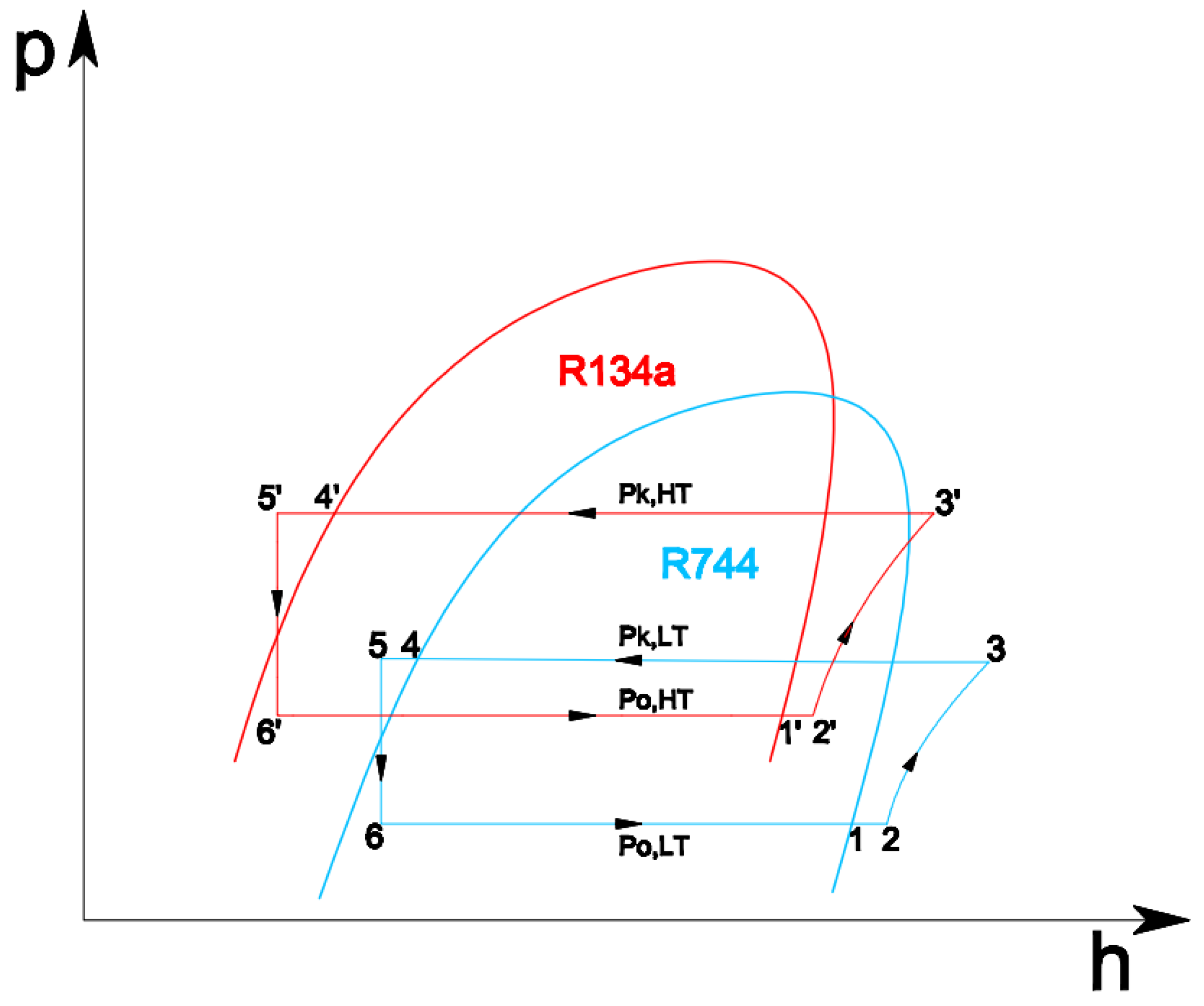
2.1. System Parameters and Design
2.2. Design of Experiments for Taguchi and ANOVA Analysis
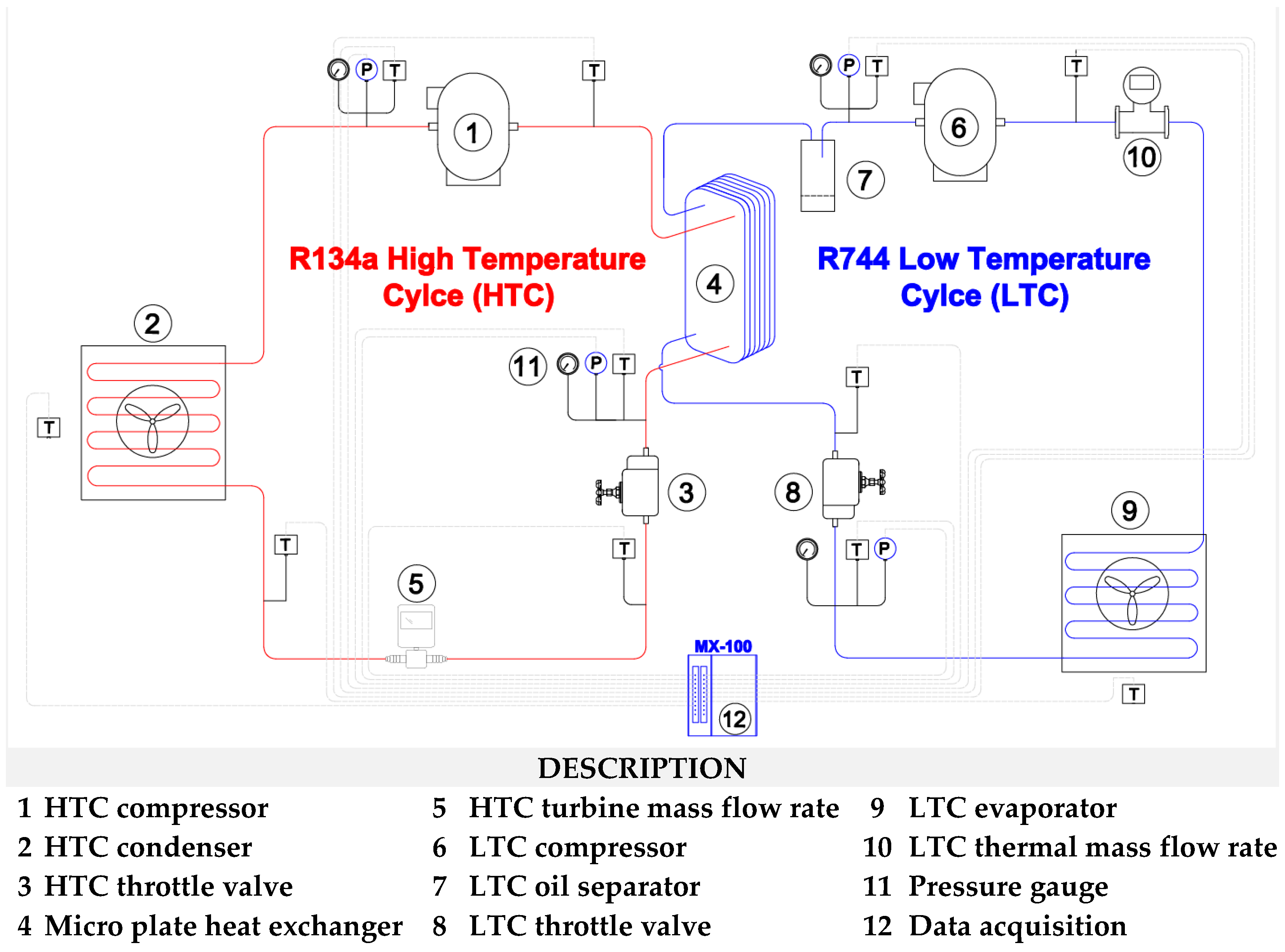
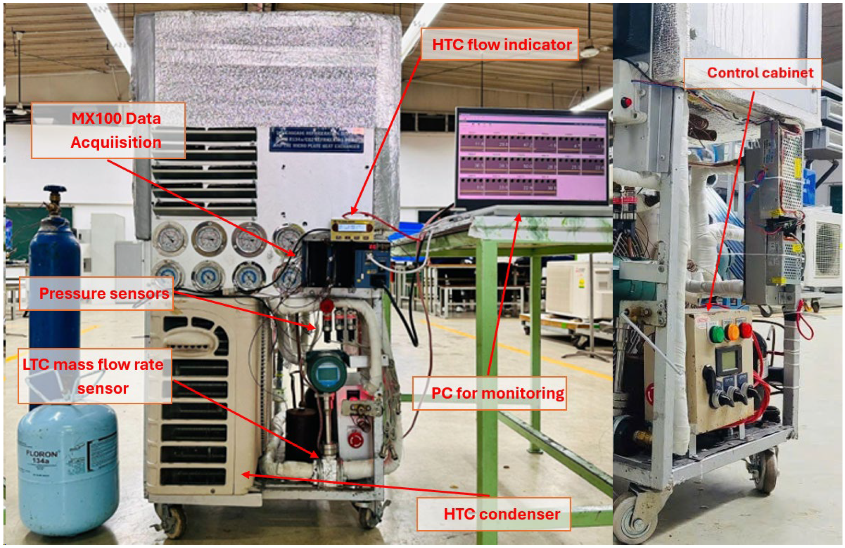
2.3. Experimental Setup
3. Results and Discussion
3.1. Taguchi and ANOVA Theory Calculation Results
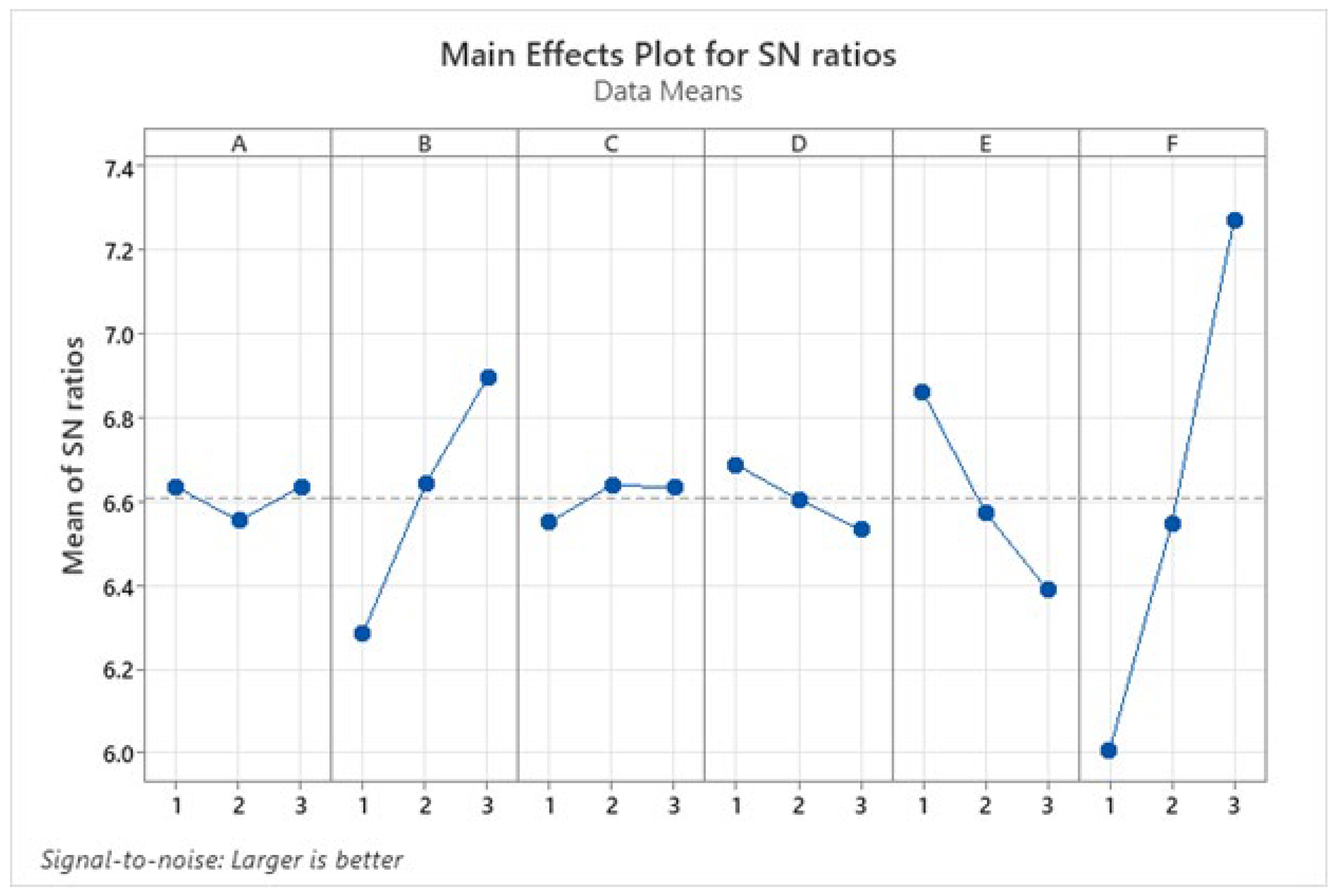
3.2. Taguchi and ANOVA Calculation Results in Experiment
3.3. Predicting COP Using Linear Regression
- In theory: COP = 1.9008 − 0.01491A + 0.07763B + 0.02759C + 0.00272D − 0.04950E + 0.14946F.
- With R2 = 0.9745.
- In actual: COP = 1.8126 + 0.0029A + 0.0754B + 0.0092C − 0.0191D − 0.0582E + 0.1562F.
- With R2 = 0.9383.
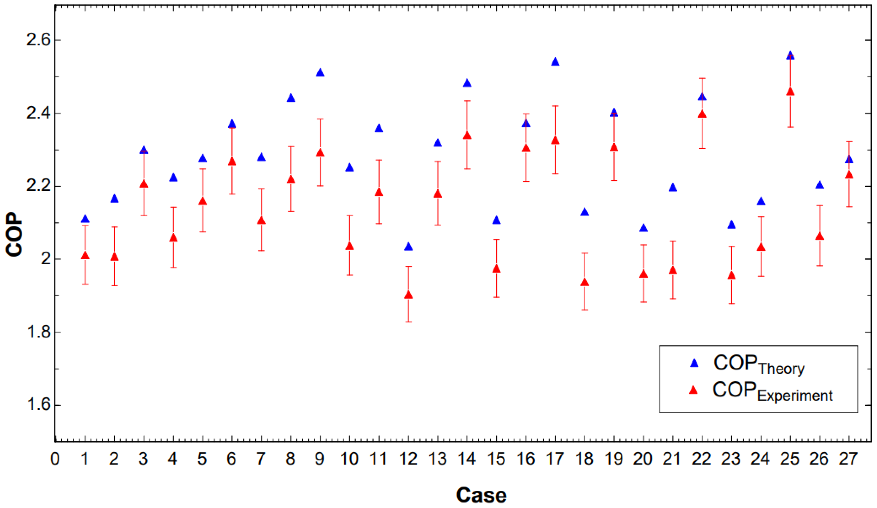
3.4. Verify
4. Conclusions
Author Contributions
Funding
Data Availability Statement
Conflicts of Interest
Abbreviations
| The absolute temperature (°C) | |
| Mass flow rate (kg/s) | |
| Work of adiabatic compression (W) | |
| Coefficient of performance | |
| Mean square | |
| Mean square error | |
| i | Experiment number |
| The data observed in experiment number i | |
| The i-th response value | |
| The number of the levels | |
| Cooling capacity (W) | |
| Condensing capacity (W) | |
| Enthalpy of fluid (kJ/kg) | |
| The signal to noise | |
| The total degree of freedom | |
| n | The number of experiments |
| The average response value | |
| F | The F_value |
| The number of factors | |
| Tsh_R744 | Superheating temperature of low temperature cycle () |
| Tsc_R744 | Subcooling temperature of low temperature cycle () |
| Te_R744 | Evaporating temperature of low temperature cycle () |
| Tc_R744 | Condensing temperature of low temperature cycle () |
| Tsh_R134a | Superheating temperature of high temperature cycle () |
| Tsc_R134a | Subcooling temperature of high temperature cycle () |
| Te_R134a | Evaporating temperature of high temperature cycle () |
| Tc_R134a | Condensing temperature of high temperature cycle () |
| LTC | Low temperature cycle |
| HTC | High temperature cycle |
References
- Sanz-Kock, C.; Llopis, R.; Sánchez, D.; Cabello, R.; Torrella, E. Experimental evaluation of a R134a/CO2 cascade refrigeration plant. Appl. Therm. Eng. 2014, 73, 41–50. [Google Scholar] [CrossRef]
- Getu, H.M.; Bansal, P.K. Thermodynamic analysis of an R744–R717 cascade refrigeration system. Int. J. Refrig. 2008, 31, 45–54. [Google Scholar] [CrossRef]
- Dubey, A.M.; Kumar, S.; Agrawal, G.D. Thermodynamic analysis of a transcritical CO2/propylene (R744–R1270) cascade system for cooling and heating applications. Energy Convers. Manag. 2014, 86, 774–783. [Google Scholar] [CrossRef]
- Dubey, A.M.; Agrawal, G.D.; Kumar, S. Thermodynamic analysis of a transcritical CO2/propylene cascade system with split unit in HT cycle. J. Braz. Soc. Mech. Sci. Eng. 2014, 37, 1365–1378. [Google Scholar] [CrossRef]
- Lee, T.-S.; Liu, C.-H.; Chen, T.-W. Thermodynamic analysis of optimal condensing temperature of cascade-condenser in CO2/NH3 cascade refrigeration systems. Int. J. Refrig. 2006, 29, 1100–1108. [Google Scholar] [CrossRef]
- Amaris, C.; Tsamos, K.M.; Tassou, S.A. Analysis of an R744 typical booster configuration, an R744 parallel-compressor booster configuration and an R717/R744 cascade refrigeration system for retail food applications. Part 1: Thermodynamic analysis. Energy Procedia 2019, 161, 259–267. [Google Scholar] [CrossRef]
- Massuchetto, L.H.P.; do Nascimento, R.B.C.; de Carvalho, S.M.R.; de Araújo, H.V.; d’Angelo, J.V.H. Thermodynamic performance evaluation of a cascade refrigeration system with mixed refrigerants: R744/R1270, R744/R717 and R744/RE170. Int. J. Refrig. 2019, 106, 201–212. [Google Scholar] [CrossRef]
- Messineo, A. R744-R717 Cascade Refrigeration System: Performance Evaluation compared with a HFC Two-Stage System. Energy Procedia 2012, 14, 56–65. [Google Scholar] [CrossRef]
- Tsamos, K.M.; Amaris, C.; Mylona, Z.; Tassou, S. Analysis of Typical Booster Configuration, Parallel-Compressor Booster Configuration and R717/R744 Cascade Refrigeration System for Food Retail Applications. Part 2: Energy Performance in Various Climate Conditions. Energy Procedia 2019, 161, 268–274. [Google Scholar] [CrossRef]
- Akan, A.E.; Ünal, F.; Özkan, D.B. Investigation of efficiency of R717 refrigerant single stage cooling system and R717/R744 refrigerant cascade cooling system. Turk. J. Eng. 2021, 5, 58–64. [Google Scholar] [CrossRef]
- Jeon, M.-J. Experimental Analysis of the R744/R404A Cascade Refrigeration System with Internal Heat Exchanger. Part 1: Coefficient of Performance Characteristics. Energies 2021, 14, 6003. [Google Scholar] [CrossRef]
- Jeon, M.-J. Experimental Analysis of the R744/R404A Cascade Refrigeration System with Internal Heat Exchanger. Part 2: Exergy Characteristics. Energies 2022, 15, 1251. [Google Scholar] [CrossRef]
- Son, C.-H.; Moon, C.-G. Performance analysis of a R744 and R404A cascade refrigeration system with internal heat exchanger. J. Power Syst. Eng. 2012, 16, 38–43. [Google Scholar] [CrossRef]
- Oh, H.-K.; Son, C.-H.; Jo, H.; Jeon, M.-J. Mass flow rate ratio analysis for optimal refrigerant charge of a R744 and R404A cascade refrigeration system. J. Korean Soc. Mar. Eng. 2013, 37, 575–581. [Google Scholar] [CrossRef]
- Song, Y.; Li, D.; Yang, D.; Jin, L.; Cao, F.; Wang, X. Performance comparison between the combined R134a/CO2 heat pump and cascade R134a/R744 heat pump for space heating. Int. J. Refrig. 2017, 74, 592–605. [Google Scholar] [CrossRef]
- Wang, B.; Wu, H.; Li, J.; Xing, Z. Experimental investigation on the performance of NH3/CO2 cascade refrigeration system with twin-screw compressor. Int. J. Refrig. 2009, 32, 1358–1365. [Google Scholar] [CrossRef]
- Queiroz, M.V.A.; Panato, V.H.; Antunes, A.H.P.; Parise, J.A.R. Experimental comparison of a cascade refrigeration system operating with R744/R134a and R744/R404A. In Proceedings of the International Refrigeration and Air Conditioning Conference, West Lafayette, IN, USA, 11–14 July 2016; p. 1785. [Google Scholar]
- Dopazo, J.A.; Fernández-Seara, J. Experimental evaluation of a cascade refrigeration system prototype with CO2 and NH3 for freezing process applications. Int. J. Refrig. 2011, 34, 257–267. [Google Scholar] [CrossRef]
- Bhattacharyya, S.; Mukhopadhyay, S.; Kumar, A.; Khurana, R.K.; Sarkar, J. Optimization of a CO2–C3H8 cascade system for refrigeration and heating. Int. J. Refrig. 2005, 28, 1284–1292. [Google Scholar] [CrossRef]
- Ma, M.; Yu, J.; Wang, X. Performance evaluation and optimal configuration analysis of a CO2/NH3 cascade refrigeration system with falling film evaporator–condenser. Energy Convers. Manag. 2014, 79, 224–231. [Google Scholar] [CrossRef]
- Dopazo, J.A.; Fernández-Seara, J.; Sieres, J.; Uhía, F.J. Theoretical analysis of a CO2–NH3 cascade refrigeration system for cooling applications at low temperatures. Appl. Therm. Eng. 2009, 29, 1577–1583. [Google Scholar] [CrossRef]
- Bhattacharyya, S.; Garai, A.; Sarkar, J. Thermodynamic analysis and optimization of a novel N2O–CO2 cascade system for refrigeration and heating. Int. J. Refrig. 2009, 32, 1077–1084. [Google Scholar] [CrossRef]
- Yari, M.; Mahmoudi, S.M.S. Thermodynamic analysis and optimization of novel ejector-expansion TRCC (transcritical CO2) cascade refrigeration cycles (Novel transcritical CO2 cycle). Energy 2011, 36, 6839–6850. [Google Scholar] [CrossRef]
- Cabello, R.; Andreu-Nácher, A.; Sánchez, D.; Llopis, R.; Vidan-Falomir, F. Energy Comparison Based on Experimental Results of a Cascade Refrigeration System Pairing R744 With R134a, R1234ze(E) and the Natural Refrigerants R290, R1270, R600a. Int. J. Refrig. 2023, 148, 131–142. [Google Scholar] [CrossRef]
- Zhao, Z.; Luo, J.; Song, Q.; Yang, K.; Wang, Q.; Chen, G. Theoretical Investigation and Comparative Analysis of the Linde–Hampson Refrigeration System Using Eco-friendly Zeotropic Refrigerants Based on R744/R1234ze(Z) for Freezing Process Applications. Int. J. Refrig. 2023, 145, 30–39. [Google Scholar] [CrossRef]
- Ojeda, F.W.A.B.; Queiroz, M.V.A.; Pico, D.F.M.; dos Reis Parise, J.A.; Bandarra Filho, E.P. Experimental Evaluation of low-GWP Refrigerants R513A, R1234yf and R436A as Alternatives for R134a in a Cascade Refrigeration Cycle With R744. Int. J. Refrig. 2022, 144, 175–187. [Google Scholar] [CrossRef]
- Ye, W.; Liu, F.; Yan, Y.; Liu, Y. Application of Response Surface Methodology and Desirabilit Approach to Optimize the Performance of an Ultra-low Temperature Cascade Refrigeration System. Appl. Therm. Eng. 2024, 239, 122130. [Google Scholar] [CrossRef]
- Rodríguez-Jara, E.Á.; Sánchez-De-La-Flor, F.J.; Expósito-Carrillo, J.A.; Salmerón-Lissén, J.M. Thermodynamic Analysis of Auto-cascade Refrigeration Cycles, With and Without Ejector, for Ultra Low Temperature Freezing Using a Mixture of Refrigerants R600a and R1150. Appl. Therm. Eng. 2022, 200, 117598. [Google Scholar] [CrossRef]
- Turgut, M.S.; Turgut, O.E. Comparative investigation and multi objective design optimization of R744/R717, R744/R134a and R744/R1234yf cascade rerfigeration systems. Heat Mass Transf. 2018, 55, 445–465. [Google Scholar] [CrossRef]
- Sobieraj, M. Development of novel wet sublimation cascade refrigeration system with binary mixtures of R744/R32 and R744/R290. Appl. Therm. Eng. 2021, 196, 117336. [Google Scholar] [CrossRef]
- Das, I.; Samanta, S. Comparative Energetic and Exergetic Analyses of a Cascade Refrigeration System Pairing R744 with R134a, R717, R1234yf, R600, R1234ze, R290. In Advances in Air Conditioning and Refrigeration; Springer: Singapore, 2020. [Google Scholar] [CrossRef]
- Canbolat, A.S.; Bademlioglu, A.H.; Arslanoglu, N.; Kaynakli, O. Performance optimization of absorption refrigeration systems using Taguchi, ANOVA and Grey Relational Analysis methods. J. Clean. Prod. 2019, 229, 874–885. [Google Scholar] [CrossRef]
- Kaya, A. Thermodynamical study and Taguchi optimization of a two-stage vapor compression refrigeration system. Therm. Sci. 2022, 26, 3951–3963. [Google Scholar] [CrossRef]
- Ustaoglu, A.; Kursuncu, B.; Alptekin, M.; Gok, M.S. Performance optimization and parametric evaluation of the cascade vapor compression refrigeration cycle using Taguchi and ANOVA methods. Appl. Therm. Eng. 2020, 180, 115816. [Google Scholar] [CrossRef]
- Keshtkar, M.M. Multi-objective optimization of a r744/r134a cascade refrigeration system: Exergetic, economic, environmental, and sensitive analysis (3ES). J. Therm. Eng. 2019, 5, 237–250. [Google Scholar] [CrossRef]
- Bejan, A.; Kraus, A.D. Heat Transfer Handbook; John Wiley & Sons: Hoboken, NJ, USA, 2003. [Google Scholar]

| Parameters | Value |
|---|---|
| Cooling capacity | 1000 W |
| The condensing temperature at the high temperature cycle | 38 °C |
| The evaporating temperature at the high temperature cycle | 2 °C |
| The cascade temperature difference | 4 °C |
| The evaporating temperature at the low temperature cycle | −25 °C |
| The superheating at the high temperature cycle | 8 °C |
| The superheating at the low temperature cycle | 7 °C |
| The subcooling at the high temperature cycle | 8 °C |
| The subcooling at the low temperature cycle | 7 °C |
| The mass flow rate of the high temperature cycle | 27.7 kg·h−1 |
| The mass flow rate of the low temperature cycle | 15.8 kg·h−1 |
| Parameters Factors | Levels | ||
|---|---|---|---|
| 1 | 2 | 3 | |
| A: Superheating temperature of low temperature cycle (°C) | 5 | 6 | 7 |
| B: Evaporating temperature of high temperature cycle (°C) | 1 | 3 | 5 |
| C: Subcooling temperature of low temperature cycle (°C) | 2 | 3 | 4 |
| D: Subcooling temperature of high temperature cycle (°C) | 4 | 5 | 6 |
| E: Condensing temperature of low temperature cycle (°C) | 6 | 7 | 8 |
| F: Evaporating temperature of low temperature cycle (°C) | −29 | −26 | −23 |
| Factors | L27 | |||||||||||
|---|---|---|---|---|---|---|---|---|---|---|---|---|
| No. | A | B | C | D | E | F | P1 | P2 | P3 | P4 | P5 | P6 |
| 1 | 5 | 1 | 2 | 4 | 6 | −29 | 1 | 1 | 1 | 1 | 1 | 1 |
| 2 | 5 | 1 | 2 | 4 | 7 | −26 | 1 | 1 | 1 | 1 | 2 | 2 |
| 3 | 5 | 1 | 2 | 4 | 8 | −23 | 1 | 1 | 1 | 1 | 3 | 3 |
| 4 | 5 | 3 | 3 | 5 | 6 | −29 | 1 | 2 | 2 | 2 | 1 | 1 |
| 5 | 5 | 3 | 3 | 5 | 7 | −26 | 1 | 2 | 2 | 2 | 2 | 2 |
| 6 | 5 | 3 | 3 | 5 | 8 | −23 | 1 | 2 | 2 | 2 | 3 | 3 |
| 7 | 5 | 5 | 4 | 6 | 6 | −29 | 1 | 3 | 3 | 3 | 1 | 1 |
| 8 | 5 | 5 | 4 | 6 | 7 | −26 | 1 | 3 | 3 | 3 | 2 | 2 |
| 9 | 5 | 5 | 4 | 6 | 8 | −23 | 1 | 3 | 3 | 3 | 3 | 3 |
| 10 | 6 | 1 | 3 | 6 | 6 | −26 | 2 | 1 | 2 | 3 | 1 | 2 |
| 11 | 6 | 1 | 3 | 6 | 7 | −23 | 2 | 1 | 2 | 3 | 2 | 3 |
| 12 | 6 | 1 | 3 | 6 | 8 | −29 | 2 | 1 | 2 | 3 | 3 | 1 |
| 13 | 6 | 3 | 4 | 4 | 6 | −26 | 2 | 2 | 3 | 1 | 1 | 2 |
| 14 | 6 | 3 | 4 | 4 | 7 | −23 | 2 | 2 | 3 | 1 | 2 | 3 |
| 15 | 6 | 3 | 4 | 4 | 8 | −29 | 2 | 2 | 3 | 1 | 3 | 1 |
| 16 | 6 | 5 | 2 | 5 | 6 | −26 | 2 | 3 | 1 | 2 | 1 | 2 |
| 17 | 6 | 5 | 2 | 5 | 7 | −23 | 2 | 3 | 1 | 2 | 2 | 3 |
| 18 | 6 | 5 | 2 | 5 | 8 | −29 | 2 | 3 | 1 | 2 | 3 | 1 |
| 19 | 7 | 1 | 4 | 5 | 6 | −23 | 3 | 1 | 3 | 2 | 1 | 3 |
| 20 | 7 | 1 | 4 | 5 | 7 | −29 | 3 | 1 | 3 | 2 | 2 | 1 |
| 21 | 7 | 1 | 4 | 5 | 8 | −26 | 3 | 1 | 3 | 2 | 3 | 2 |
| 22 | 7 | 3 | 2 | 6 | 6 | −23 | 3 | 2 | 1 | 3 | 1 | 3 |
| 23 | 7 | 3 | 2 | 6 | 7 | −29 | 3 | 2 | 1 | 3 | 2 | 1 |
| 24 | 7 | 3 | 2 | 6 | 8 | −26 | 3 | 2 | 1 | 3 | 3 | 2 |
| 25 | 7 | 5 | 3 | 4 | 6 | −23 | 3 | 3 | 2 | 1 | 1 | 3 |
| 26 | 7 | 5 | 3 | 4 | 7 | −29 | 3 | 3 | 2 | 1 | 2 | 1 |
| 27 | 7 | 5 | 3 | 4 | 8 | −26 | 3 | 3 | 2 | 1 | 3 | 2 |
| Device | Accuracy | Range | Manufacturer |
|---|---|---|---|
| Thermocouples—T type | ±0.1 °C | −270–400 °C | Omega (Michigan City, IN, USA) |
| Clamp meter | ±2%FS | 0–600 A | Hioki (Nagano, Japan) |
| Digital acquisition | - | 20 channels | Yokogawa (Tokyo, Japan) |
| Pressure sensor | ±0.5%FS | 0–100 bars | Sensys (Gyeonggi-do, Republic of Korea) |
| Turbine flow rate meter | ±0.5% | 400 to 5000 L/h | Digital Flow Co., Ltd. (Chungcheongbuk-do, Republic of Korea) |
| Thermal mass flow gas meter | ±1.5% | 0.5 to 28 Nm3/h | Anhui Jujie (Anhui, China) |
| Components | Specifications | Manufacturer |
|---|---|---|
| LTC Compressor | Hermetic Compressor | Sanden (Shandong, China) Model SRcACA; No. 6456 |
| HTC Compressor | Hermetic Compressor | Kulthorn (Bangkok, Thailand); Model AE2428ZK-SR |
| HTC Condenser | Finned Tube Heat Exchanger | Samsung (Chonburi, Thailand); Model AR10MVFHGWKXSVHeat Transfer Area: 2.8 m2 |
| Cascade Heat Exchanger | Welded Plate Heat Exchanger | Danfoss (Nordborg, Denmark) Model D22/16; No. 021H1297 |
| Case | A | B | C | D | E | F | COPtrial1 | COPtrial2 | COPtrial3 | COPmean |
|---|---|---|---|---|---|---|---|---|---|---|
| 1 | 5 | 1 | 2 | 4 | 6 | −29 | 2.153 | 2.138 | 2.074 | 2.122 |
| 2 | 5 | 1 | 2 | 4 | 7 | −26 | 2.254 | 2.133 | 2.114 | 2.167 |
| 3 | 5 | 1 | 2 | 4 | 8 | −23 | 2.360 | 2.284 | 2.259 | 2.301 |
| 4 | 5 | 3 | 3 | 5 | 6 | −29 | 2.259 | 2.241 | 2.174 | 2.225 |
| 5 | 5 | 3 | 3 | 5 | 7 | −26 | 2.368 | 2.244 | 2.222 | 2.278 |
| 6 | 5 | 3 | 3 | 5 | 8 | −23 | 2.485 | 2.354 | 2.276 | 2.372 |
| 7 | 5 | 5 | 4 | 6 | 6 | −29 | 2.368 | 2.247 | 2.228 | 2.281 |
| 8 | 5 | 5 | 4 | 6 | 7 | −26 | 2.487 | 2.459 | 2.384 | 2.443 |
| 9 | 5 | 5 | 4 | 6 | 8 | −23 | 2.613 | 2.479 | 2.447 | 2.513 |
| 10 | 6 | 1 | 3 | 6 | 6 | −26 | 2.343 | 2.269 | 2.148 | 2.253 |
| 11 | 6 | 1 | 3 | 6 | 7 | −23 | 2.456 | 2.326 | 2.299 | 2.36 |
| 12 | 6 | 1 | 3 | 6 | 8 | −29 | 2.079 | 2.019 | 2.011 | 2.036 |
| 13 | 6 | 3 | 4 | 4 | 6 | −26 | 2.431 | 2.303 | 2.227 | 2.32 |
| 14 | 6 | 3 | 4 | 4 | 7 | −23 | 2.551 | 2.516 | 2.384 | 2.484 |
| 15 | 6 | 3 | 4 | 4 | 8 | −29 | 2.154 | 2.09 | 2.079 | 2.108 |
| 16 | 6 | 5 | 2 | 5 | 6 | −26 | 2.469 | 2.34 | 2.314 | 2.374 |
| 17 | 6 | 5 | 2 | 5 | 7 | −23 | 2.594 | 2.558 | 2.474 | 2.542 |
| 18 | 6 | 5 | 2 | 5 | 8 | −29 | 2.178 | 2.164 | 2.052 | 2.131 |
| 19 | 7 | 1 | 4 | 5 | 6 | −23 | 2.520 | 2.385 | 2.304 | 2.403 |
| 20 | 7 | 1 | 4 | 5 | 7 | −29 | 2.133 | 2.07 | 2.059 | 2.087 |
| 21 | 7 | 1 | 4 | 5 | 8 | −26 | 2.233 | 2.214 | 2.148 | 2.198 |
| 22 | 7 | 3 | 2 | 6 | 6 | −23 | 2.565 | 2.429 | 2.347 | 2.447 |
| 23 | 7 | 3 | 2 | 6 | 7 | −29 | 2.159 | 2.096 | 2.034 | 2.096 |
| 24 | 7 | 3 | 2 | 6 | 8 | −26 | 2.262 | 2.143 | 2.076 | 2.16 |
| 25 | 7 | 5 | 3 | 4 | 6 | −23 | 2.667 | 2.526 | 2.488 | 2.560 |
| 26 | 7 | 5 | 3 | 4 | 7 | −29 | 2.239 | 2.221 | 2.156 | 2.205 |
| 27 | 7 | 5 | 3 | 4 | 8 | −26 | 2.347 | 2.274 | 2.204 | 2.275 |
| No | A | B | C | D | E | F |
|---|---|---|---|---|---|---|
| 1 | 7.224 | 6.892 | 7.063 | 7.150 | 7.341 | 6.618 |
| 2 | 7.174 | 7.131 | 7.163 | 7.182 | 7.198 | 7.131 |
| 3 | 7.102 | 7.476 | 7.274 | 7.168 | 6.960 | 7.751 |
| Delta | 0.122 | 0.584 | 0.211 | 0.031 | 0.381 | 1.134 |
| Rank | 5 | 2 | 4 | 6 | 3 | 1 |
| Source | DF | Adj SS | Adj MS | F-Value | p-Value |
|---|---|---|---|---|---|
| Regression | 6 | 0.572522 | 0.095420 | 127.39 | 0.000 |
| A | 1 | 0.004000 | 0.004000 | 5.34 | 0.032 |
| B | 1 | 0.108474 | 0.108474 | 144.82 | 0.000 |
| C | 1 | 0.013704 | 0.013704 | 18.30 | 0.000 |
| D | 1 | 0.000133 | 0.000133 | 0.18 | 0.678 |
| E | 1 | 0.044104 | 0.044104 | 58.88 | 0.000 |
| F | 1 | 0.402105 | 0.402105 | 536.82 | 0.000 |
| Error | 20 | 0.014981 | 0.000749 | ||
| Total | 26 | 0.587503 |
| Source | Var | % of Total | SE Var | Z-Value | p-Value |
|---|---|---|---|---|---|
| A | 0.000158 | 0.49% | 0.000231 | 0.682521 | 0.247 |
| B | 0.006032 | 18.65% | 0.006104 | 0.988209 | 0.162 |
| C | 0.000692 | 2.14% | 0.000764 | 0.905338 | 0.183 |
| D | 0.000000 | 0.00% | * | * | * |
| E | 0.002441 | 7.54% | 0.002513 | 0.971328 | 0.166 |
| F | 0.022382 | 69.18% | 0.022454 | 0.996797 | 0.159 |
| Error | 0.000647 | 2.00% | 0.000229 | 2.828427 | 0.002 |
| Total | 0.032351 | ||||
| 2 Log likelihood = −79.307472 | |||||
| Thermodynamic State Point | Temperature (°C) | Pressure (bar) |
|---|---|---|
| 1 | −29 | 14.68 |
| 2 | −24 | 14.68 |
| 3 | 51.2 | 40.62 |
| 4 | 5.9 | 40.61 |
| 5 | 3.4 | 40.61 |
| 6 | −29 | 14.70 |
| 1′ | 0.76 | 3.02 |
| 2′ | 9.9 | 3.02 |
| 3′ | 49.3 | 8.81 |
| 4′ | 34.7 | 8.79 |
| 5′ | 30.6 | 8.79 |
| 6′ | 1.1 | 3.03 |
| Case | A | B | C | D | E | F | COPmean |
|---|---|---|---|---|---|---|---|
| 1 | 5 | 1 | 2 | 4 | 6 | −29 | 2.012 |
| 2 | 5 | 1 | 2 | 4 | 7 | −26 | 2.008 |
| 3 | 5 | 1 | 2 | 4 | 8 | −23 | 2.208 |
| 4 | 5 | 3 | 3 | 5 | 6 | −29 | 2.060 |
| 5 | 5 | 3 | 3 | 5 | 7 | −26 | 2.161 |
| 6 | 5 | 3 | 3 | 5 | 8 | −23 | 2.269 |
| 7 | 5 | 5 | 4 | 6 | 6 | −29 | 2.108 |
| 8 | 5 | 5 | 4 | 6 | 7 | −26 | 2.22 |
| 9 | 5 | 5 | 4 | 6 | 8 | −23 | 2.293 |
| 10 | 6 | 1 | 3 | 6 | 6 | −26 | 2.038 |
| 11 | 6 | 1 | 3 | 6 | 7 | −23 | 2.185 |
| 12 | 6 | 1 | 3 | 6 | 8 | −29 | 1.904 |
| 13 | 6 | 3 | 4 | 4 | 6 | −26 | 2.181 |
| 14 | 6 | 3 | 4 | 4 | 7 | −23 | 2.341 |
| 15 | 6 | 3 | 4 | 4 | 8 | −29 | 1.975 |
| 16 | 6 | 5 | 2 | 5 | 6 | −26 | 2.306 |
| 17 | 6 | 5 | 2 | 5 | 7 | −23 | 2.327 |
| 18 | 6 | 5 | 2 | 5 | 8 | −29 | 1.979 |
| 19 | 7 | 1 | 4 | 5 | 6 | −23 | 2.308 |
| 20 | 7 | 1 | 4 | 5 | 7 | −29 | 1.961 |
| 21 | 7 | 1 | 4 | 5 | 8 | −26 | 1.971 |
| 22 | 7 | 3 | 2 | 6 | 6 | −23 | 2.400 |
| 23 | 7 | 3 | 2 | 6 | 7 | −29 | 1.957 |
| 24 | 7 | 3 | 2 | 6 | 8 | −26 | 2.035 |
| 25 | 7 | 5 | 3 | 4 | 6 | −23 | 2.461 |
| 26 | 7 | 5 | 3 | 4 | 7 | −29 | 2.065 |
| 27 | 7 | 5 | 3 | 4 | 8 | −26 | 2.233 |
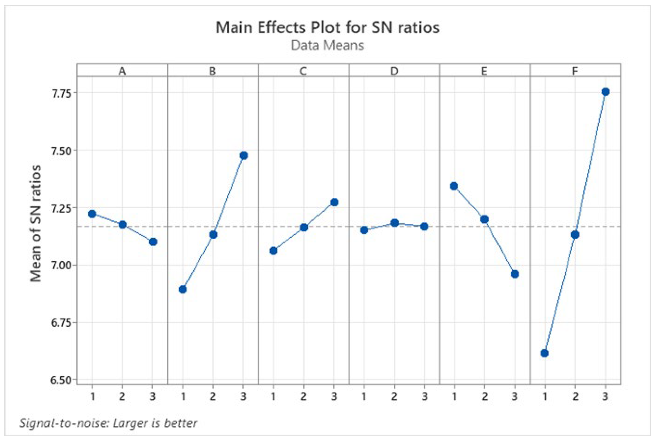
| Larger Is Better | ||||||
|---|---|---|---|---|---|---|
| Level | A | B | C | D | E | F |
| 1 | 6.634 | 6.287 | 6.551 | 6.687 | 6.859 | 6.007 |
| 2 | 6.554 | 6.641 | 6.639 | 6.604 | 6.574 | 6.548 |
| 3 | 6.635 | 6.895 | 6.633 | 6.532 | 6.389 | 7.268 |
| Delta | 0.081 | 0.608 | 0.088 | 0.155 | 0.470 | 1.261 |
| Rank | 6 | 2 | 5 | 4 | 3 | 1 |
| Source | DF | Adj SS | Adj MS | F-Value | p-Value |
|---|---|---|---|---|---|
| Regression | 6 | 0.610443 | 0.101741 | 50.71 | 0.000 |
| A | 1 | 0.000150 | 0.000150 | 0.07 | 0.787 |
| B | 1 | 0.102303 | 0.102303 | 50.99 | 0.000 |
| C | 1 | 0.001531 | 0.001531 | 0.76 | 0.393 |
| D | 1 | 0.006574 | 0.006574 | 3.28 | 0.085 |
| E | 1 | 0.060900 | 0.060900 | 30.35 | 0.000 |
| F | 1 | 0.438984 | 0.438984 | 218.80 | 0.000 |
| Error | 20 | 0.040127 | 0.002006 | ||
| Total | 26 | 0.650571 |
| Source | Var | % of Total | SE Var | Z-Value | p-Value |
|---|---|---|---|---|---|
| A | 0.000000 | 0.00% | * | * | * |
| B | 0.005508 | 15.62% | 0.005730 | 0.961380 | 0.168 |
| C | 0.000000 | 0.00% | * | * | * |
| D | 0.000145 | 0.41% | 0.000373 | 0.388319 | 0.349 |
| E | 0.003227 | 9.15% | 0.003449 | 0.935750 | 0.175 |
| F | 0.024392 | 69.18% | 0.024613 | 0.991024 | 0.161 |
| Error | 0.001987 | 5.64% | 0.000662 | 3.000000 | 0.001 |
| Total | 0.035260 |
| Case | COPTheory | COPExperiment | Predicted COPActual | Difference (%) |
|---|---|---|---|---|
| 1 | 2.122 | 2.012 | 1.979 | 1.640 |
| 2 | 2.167 | 2.008 | 2.077 | 3.436 |
| 3 | 2.301 | 2.208 | 2.175 | 1.495 |
| 4 | 2.225 | 2.06 | 2.045 | 0.752 |
| 5 | 2.278 | 2.161 | 2.143 | 0.856 |
| 6 | 2.372 | 2.269 | 2.241 | 1.256 |
| 7 | 2.281 | 2.108 | 2.110 | 0.095 |
| 8 | 2.443 | 2.22 | 2.208 | 0.541 |
| 9 | 2.513 | 2.293 | 2.306 | 0.567 |
| 10 | 2.253 | 2.038 | 2.109 | 3.489 |
| 11 | 2.360 | 2.185 | 2.207 | 1.011 |
| 12 | 2.036 | 1.904 | 1.837 | 3.545 |
| 13 | 2.320 | 2.181 | 2.232 | 2.334 |
| 14 | 2.484 | 2.341 | 2.330 | 0.474 |
| 15 | 2.108 | 1.975 | 1.959 | 0.795 |
| 16 | 2.374 | 2.306 | 2.270 | 1.570 |
| 17 | 2.542 | 2.327 | 2.368 | 1.753 |
| 18 | 2.131 | 1.939 | 1.997 | 3.002 |
| 19 | 2.403 | 2.308 | 2.297 | 0.498 |
| 20 | 2.087 | 1.961 | 1.926 | 1.790 |
| 21 | 2.198 | 1.971 | 2.024 | 2.684 |
| 22 | 2.447 | 2.4 | 2.334 | 2.733 |
| 23 | 2.096 | 1.957 | 1.964 | 0.347 |
| 24 | 2.160 | 2.035 | 2.062 | 1.317 |
| 25 | 2.560 | 2.461 | 2.457 | 0.154 |
| 26 | 2.205 | 2.065 | 2.087 | 1.046 |
| 27 | 2.275 | 2.233 | 2.185 | 2.167 |
| Factor | Trial 1 | Trial 2 | Trial 3 | Trial 4 | Trial 5 |
|---|---|---|---|---|---|
| A | 6.38 | 6.43 | 6.35 | 6.57 | 6.3 |
| B | 5 | 5 | 5 | 5 | 5 |
| C | 2.88 | 2.93 | 2.75 | 3.07 | 2.8 |
| D | 4.14 | 3.89 | 4.06 | 4.19 | 4.01 |
| E | 7 | 7 | 7 | 7 | 7 |
| F | −23 | −23 | −23 | −23 | −23 |
| COP | 2.475 | 2.477 | 2.473 | 2.484 | 2.48 |
Disclaimer/Publisher’s Note: The statements, opinions and data contained in all publications are solely those of the individual author(s) and contributor(s) and not of MDPI and/or the editor(s). MDPI and/or the editor(s) disclaim responsibility for any injury to people or property resulting from any ideas, methods, instructions or products referred to in the content. |
© 2025 by the authors. Licensee MDPI, Basel, Switzerland. This article is an open access article distributed under the terms and conditions of the Creative Commons Attribution (CC BY) license (https://creativecommons.org/licenses/by/4.0/).
Share and Cite
Dang, T.; Nguyen, H.; Dang, H.-S. Thermal Parameters Optimization of the R744/R134a Cascade Refrigeration Cycle Using Taguchi and ANOVA Methods. Processes 2025, 13, 1210. https://doi.org/10.3390/pr13041210
Dang T, Nguyen H, Dang H-S. Thermal Parameters Optimization of the R744/R134a Cascade Refrigeration Cycle Using Taguchi and ANOVA Methods. Processes. 2025; 13(4):1210. https://doi.org/10.3390/pr13041210
Chicago/Turabian StyleDang, Thanhtrung, Hoangtuan Nguyen, and Hung-Son Dang. 2025. "Thermal Parameters Optimization of the R744/R134a Cascade Refrigeration Cycle Using Taguchi and ANOVA Methods" Processes 13, no. 4: 1210. https://doi.org/10.3390/pr13041210
APA StyleDang, T., Nguyen, H., & Dang, H.-S. (2025). Thermal Parameters Optimization of the R744/R134a Cascade Refrigeration Cycle Using Taguchi and ANOVA Methods. Processes, 13(4), 1210. https://doi.org/10.3390/pr13041210