Abstract
To address the issues of cumulative plastic deformation and low-cycle fatigue cracking in ultra-high voltage (UHV) disc spring hydraulic circuit breakers under long-term cyclic high-pressure loads, which lead to internal structural changes and affect closing time stability and phase-controlled closing accuracy, this paper proposes a closing time prediction model considering the low-cycle fatigue of the operating mechanism. First, a Simulink-based simulation model of the 550 kV disc spring hydraulic operating mechanism transmission system was developed to analyze the influence of structural parameter variations on closing time under no-load conditions. Then, an objective function for judging action time stability was constructed, and the stability and influence weights of each structural parameter were calculated under different mechanical dispersion requirements using a combination of adaptive surrogate models and directional importance sampling. Results show that critical parameters such as working cylinder inner diameter, working cylinder stroke, main valve stroke, and working cylinder rod diameter significantly affect closing time, contributing approximately 25%, 20%, 15%, and 10%, respectively. Finally, a dynamic-weighted closing time prediction model was designed based on different phase-controlled accuracy requirements. Compared with no-load closing tests, under mechanical dispersion conditions of ±1 ms, ±1.5 ms, and ±2 ms, the optimized model reduced maximum deviations by 12.8%, 20.4%, and 23.3%, and narrowed fluctuation ranges by 37%, 38.3%, and 38.6%, respectively, significantly improving prediction accuracy. This work is supported by the Science and Technology Project of China Southern Power Grid (No.CGYKJXM20220346).
1. Introduction
High-voltage circuit breakers, as critical primary equipment in power systems, are mainly composed of three parts: the interrupting section, transmission section, and insulation section [1,2,3,4]. Disc spring hydraulic operating mechanisms are widely applied in the 500–1100 kV extra-high voltage field due to their compact structure and large and stable output force [5,6,7,8]. As the number of circuit breaker operations increases, the continuous accumulation of plastic deformation caused by low-cycle fatigue in its internal structure leads to structural parameter changes, indirectly affecting the closing time of the circuit breaker. This results in reduced phase-controlled closing accuracy and endangers the stable operation of high-voltage lines and power equipment [9,10,11,12].
Currently, there are few studies on the stability degradation of ultra-high voltage circuit breaker operating mechanisms caused by structural parameter changes. Traditional ultra-high voltage circuit breakers have long operation times and poor stability, leading to a closing time dispersion of up to ±10 ms [13]. With the upgrading of operating mechanisms, the use of mechanisms with higher energy density can reduce mechanical dispersion to approximately ±1 ms [14,15]. Current research mainly focuses on improving the stability of key components to enhance overall mechanism stability. Reference [16] studies mechanical characteristics through the cross-verification of experimental and simulation results, then locates fault positions by comparing fault opening waveforms. In Reference [17], structural optimization was performed by studying the fatigue life of the mechanism’s buffer, improving product quality. Reference [18] investigates stress relaxation and fault identification in operating mechanisms, validates the accuracy of dynamic models through experimental comparison, and proposes a remaining fatigue prediction model. Reference [19] integrates electrical, magnetic, dynamic operation, fluid, mechanical, pneumatic, and thermal models into a multi-physics coupling model, conducting simulations and experimental verification on a 550 kV high-voltage circuit breaker to accurately predict and optimize the dynamic characteristics of hydraulic operating mechanisms. Studies in References [20,21,22,23] focus on electric field and gas flow distribution in arc extinguishers under a given output pressure and velocity of operating mechanisms, or investigate hydraulic operating mechanism performance under specified loads [24].
Scholars have made significant achievements in quantitative methods for analyzing the stability of hydraulic systems. Bošnjak et al. [25] studied microstructural changes in stress-concentrated regions of hydraulic systems through finite element analysis, revealing the dominant factors in fatigue failure. Arsic et al. [26] conducted three-point bending tests on wheel loader booms, deeply characterizing fatigue crack propagation processes. Their research provided a new experimental approach for fatigue analysis of welded structures and highlighted the critical impact of welding material selection on mechanical performance. Liu et al. [27] investigated excavator digging processes under different working conditions, considering eccentric loads, impacts, and other factors to provide experimental data for constructing hinge point load spectra. They further predicted boom fatigue life using the discrete element method. This fatigue analysis not only explored excavator performance under real operational conditions but also evaluated the influence of different design parameters on fatigue life. Mohammad et al. [28] applied Monte Carlo simulation to quantify uncertain loads on EC460 excavator working devices under complex conditions, optimizing dipper stick structures based on these results. The optimized dipper stick demonstrated significant improvements in both mass and stress performance, further enhancing structural stability and reliability.
Although numerous studies have been conducted on disc spring hydraulic operating mechanisms, most focus on model establishment and design optimization. There is a lack of quantitative research on the low-cycle fatigue of operating mechanisms caused by frequent operations in long-term running circuit breakers, which affects the stability of closing time and hinders the implementation of phase-controlled closing. Therefore, it is critical to establish an accurate and efficient stability calculation model for operating mechanisms. Based on this, this paper first constructs a mathematical model capable of accurately describing the dynamic performance of the mechanism to analyze the operational characteristics of disc spring hydraulic operating mechanisms. Then, a stability analysis limit state function based on time-threshold judgment is established, combining the Adaptive Kriging (Adaptive Kriging, AK) surrogate model with Directional Importance Sampling (Directional Importance Sampling, DIS) to develop an efficient and accurate stability assessment method. Finally, under different mechanical dispersion requirements, the influence weight changes of each component are analyzed, constructing a closing time prediction model and comparing it with actual experimental data.
2. Model of Disc Spring Hydraulic Actuator
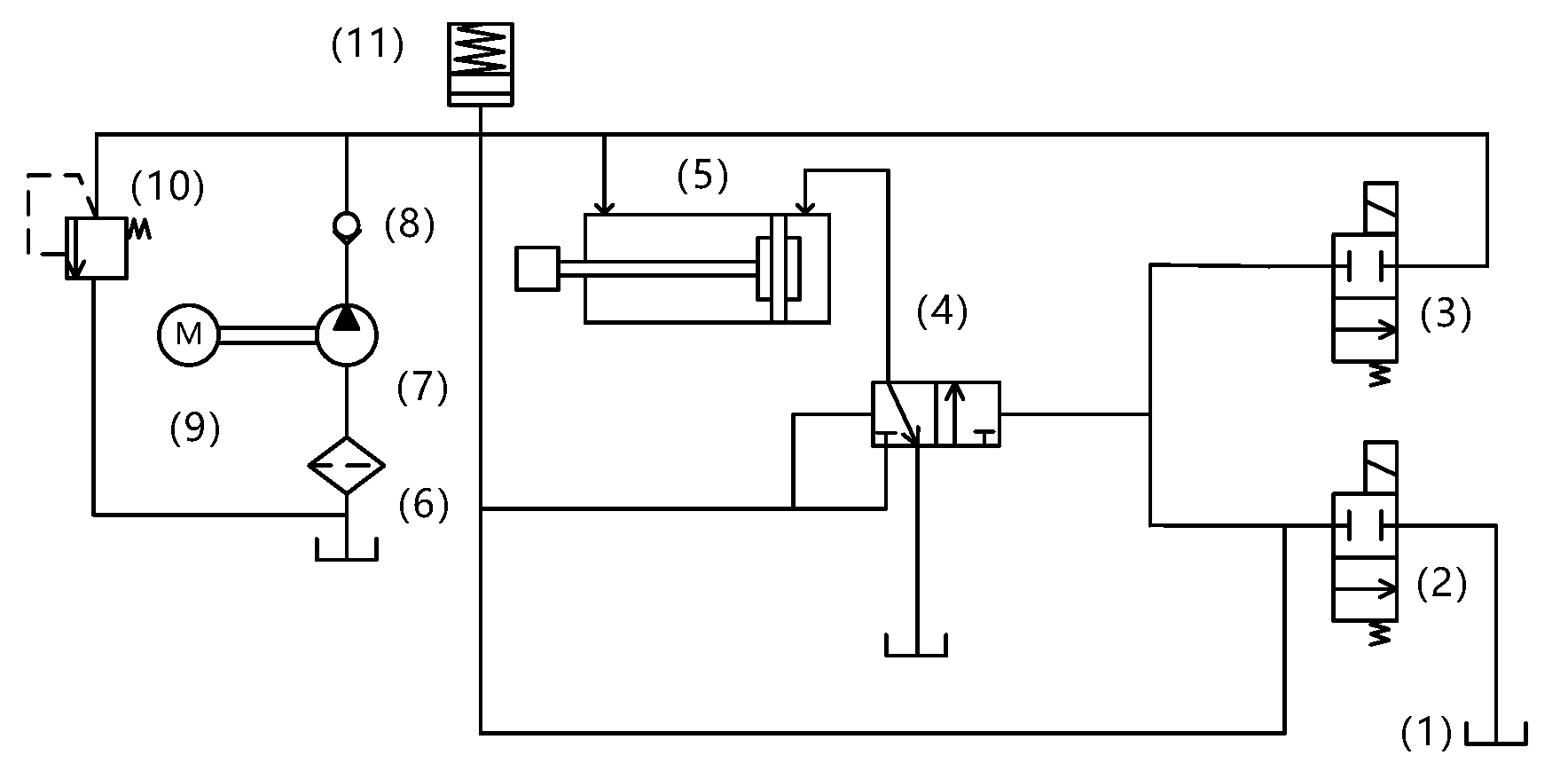
The power chain of the disc spring hydraulic operation mechanism is disc spring–solenoid valve–main valve–hydraulic cylinder, as shown in Figure 1 and Figure 2, and the parts of the structure are as follows: 1. oil cylinder; 2. opening solenoid; 3. closing solenoid; 4. main valve; 5. working cylinder; 6. filter screen; 7. hydraulic pump; 8. check valve; 9. energy storage motor; 10. relief valve; and 11. disc spring energy storage device. The working principle of the system is as follows: the energy storage motor drives the piston pump to compress the disc spring to the set stroke, and the pressure stops when the system oil pressure rises to the specified value, and the energy storage ends. When the closing signal command is issued, the closing solenoid coil is electrified, the armature drives the push rod to move, the high-pressure oil enters the main valve to make it move to the closing position, and then the high-pressure oil enters the rodless cavity of the working cylinder through the main valve, and the hydraulic pressure generated by the hydraulic pressure difference promotes the piston movement of the working cylinder, and the insulating rod connected with it pushes the contact closure of the arc extinguisher to complete the system closing operation.
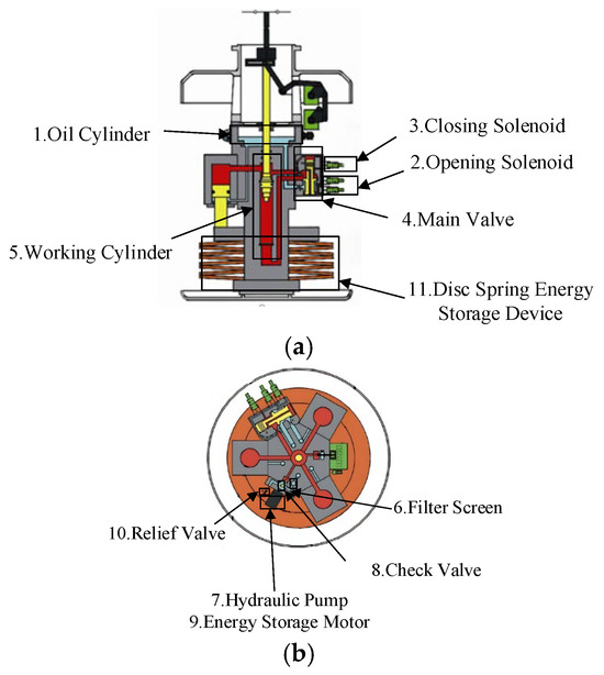
Figure 1.
Disc spring hydraulic operating system structure diagram: (a) side view and (b) top view.
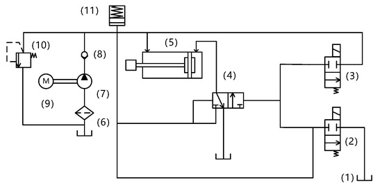
Figure 2.
Schematic diagram of the disc spring hydraulic operating mechanism.
In the process of circuit breaker closing, the hydraulic operating mechanism of the disc spring relies on the differential principle to realize the movement of the main valve and the hydraulic cylinder, and the movement energy of this process only comes from the elastic potential energy in the process of disc spring energy storage. The main structural components that affect the dynamic performance of the circuit breaker are the solenoid valve, the main valve, the working cylinder and the arc extinguishing chamber. In this paper, when establishing the action model of the mechanism, it is assumed that all parts of the system are independent [19], there is no elastic deformation [29] or bubbles in the pipe wall [30], and the upper valve is fully opened when the lower valve is acted, regardless of the friction experienced during the movement of the spool [31].
2.1. Solenoid Valve
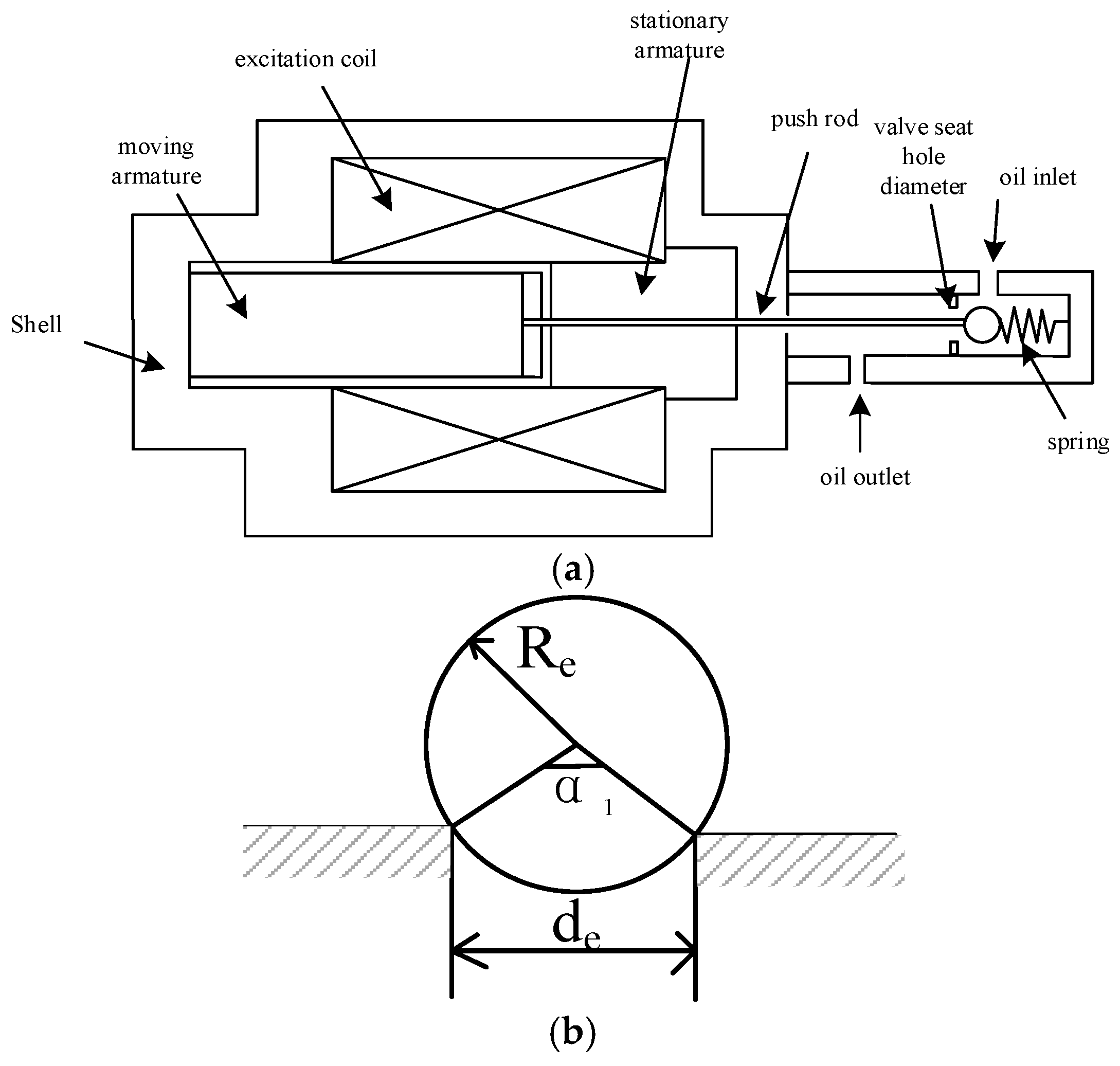
The first-stage control valve of the disc spring hydraulic operation system is the solenoid ball valve; when energized, the solenoid valve coil is charged to promote the armature movement, the ball valve is opened by the push rod to overcome the hydraulic pressure and the elastic force of the spring, the high-pressure oil passes through the solenoid valve, and when the power is lost, with the reduction of electromagnetic force, the solenoid valve is gradually closed, as shown in Figure 3.
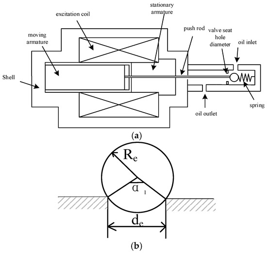
Figure 3.
Solenoid valve structure schematic: (a) cross-sectional view and (b) throttle orifice schematic diagram.
The equation for the motion of the closing solenoid valve is as follows:
where FE is the output force of the electromagnet; mc is the mass of the solenoid valve core; Fn is the viscous friction force; FT is the spring reaction force; and FY is the hydrodynamic force.
The effective area of the ball valve core is as follows:
where de is the seat hole diameter; Re is the diameter of the ball valve steel ball core; and α1 is the valve port angle.
2.2. Main Valve
The structure of the main valve is shown in Figure 4. From left to right, the force-acting surfaces of the valve core are labeled as A1, A2, and A3, with the area relationship being A1 < A2 < A3, and A1 + A2 > A3. Before the closing action, the A1 pressure surface is exposed to low-pressure oil, while A2 and A3 are maintained by high-pressure oil. When the closing signal is issued, high-pressure oil flows to the A1 surface through the closing solenoid valve. Under the effect of the area difference, the main valve core moves to the right. High-pressure oil flows into the rodless chamber of the working cylinder through port Z, and the working cylinder moves under the pressure differential, thus completing the closing operation. During the closing process, the motion equation of the main valve core is as follows:
where Pg is the high-pressure oil pressure; Fvl is the viscous friction force; FS is the steady-state liquid pressure; and mz is the mass of the main valve.
The flow rate variance of the main valve is as follows:
where Pp is the pressure at the P port of the main valve; Pz is the pressure at the Z port of the main valve; and Cd is the flow coefficient of the closing valve port.
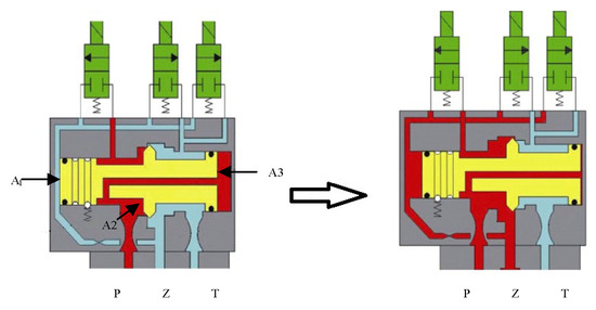
Figure 4.
Main valve structure.
Figure 4.
Main valve structure.

2.3. Working Cylinder
In the closing phase, the equation for the motion of the hydraulic cylinder is as follows:
where A4 is the area of the rod cavity, A5 is the area of the rodless cavity, Fh is the buffer force of the rod cavity, Fv2 is the viscous friction force, Fm is the load reaction force, and my is the piston mass of the working cylinder.
2.4. Loads
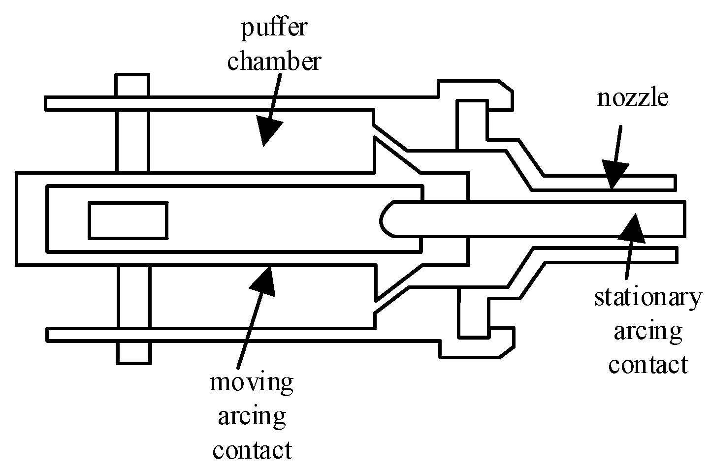
The load connected to the piston rod of the working cylinder is a compressed-air type arc extinguishing chamber, as shown in Figure 5. The load force under no-load conditions is as follows:
where Fm represents the pressure gas reaction force; Pt is the pressure of the gas in the compression chamber; P0 is the initial pressure of the compression gas; Ap is the area affected by the gas reaction force; ρ0 is the initial density of the gas in the compression chamber; κ is the specific heat capacity of the gas; V0 is the initial volume of the gas; m0 is the initial mass of the gas in the compression chamber; Vt is the volume of the compression chamber; and mt is the mass of the gas in the compression chamber.

Figure 5.
Arc extinguishing chamber structure.
The physical parameters of the four main components of the disc spring hydraulic operating mechanism are shown in the figure below. First, the solenoid valve receives a step signal, and the electromagnetic force overcomes the spring reaction force and hydraulic force, transitioning the solenoid valve from the closed state to the open state. High-pressure oil flows from the accumulator into the solenoid valve, and the spool velocity and post-opening pressure are transmitted to the main valve. The high-pressure oil enters the A1 surface of the main valve, and the total hydraulic force on the A1 and A2 surfaces of the main valve exceeds that on the A3 surface, causing the main valve to activate. The spool velocity and pressure of the main valve are then transmitted to the working cylinder. When the pressure in the rodless chamber of the working cylinder exceeds that in the rod chamber, the piston begins to move, causing the differential pressure force of the working cylinder on the load to be transmitted to the load. Concurrently, the load reaction force is transferred back to the working cylinder. The transmission chain operation process is shown in Figure 6. Boundary conditions are shown in Table 1.
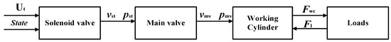
Figure 6.
Transmission chain operation process.

Table 1.
Boundary conditions.
2.5. Simulation Analysis
The closing time of the disc spring hydraulic operating system is relatively short, and the compression variation in the disc spring is minimal. During this period, it is assumed that the system’s high-pressure oil pressure remains constant. The main parameters of the model are listed in Table 2. A model of the four components is built using Simulink, and by varying the parameters, the dynamic characteristics of the operating mechanism are studied.
Table 2.
Main parameters of model.
2.5.1. Typical Working Condition Analysis
A hardware-in-the-loop simulation platform based on RT-LAB is a collection of multi-domain modeling capabilities, distributed real-time processing technology, rich I/O interfaces, and powerful API functions, which can be seamlessly integrated into the MATLAB/Simulink R2021b environment, with high-precision algorithms and powerful computing capabilities, accurate modeling and real-time simulation of the complex dynamic characteristics of the hydraulic system, and design optimization, performance evaluation, and performance evaluation of the hydraulic system. Fault diagnosis and control strategy development provide an advanced and reliable digital analysis environment. The simulation model of the hydraulic actuator of the disc spring was imported into the RT-LAB 2023.1 software for simulation and operation. The demonstration of the actual machine and the display of the simulation interface are shown in Figure 7.
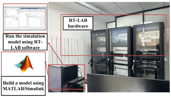
Figure 7.
Based on the RT-LAB experimental platform.
To verify the accuracy of the simulation results, we designed the layout diagram of the no-load closing test equipment as shown in Figure 8. The disc spring hydraulic operating mechanism uses an energy storage motor to charge the disc spring, and controls the directional control valve through closing and opening coils to switch between high and low pressure oil circuits, thereby completing the closing and opening operations. A dynamic characteristic tester is used to acquire closing/opening signals, an angular displacement sensor measures contact displacement, and an oscilloscope records the circuit breaker’s closing and opening current curves. The equipment arrangement is shown in Figure 8.
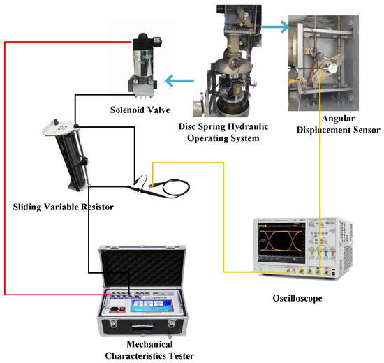
Figure 8.
No-load closing test equipment layout diagram.
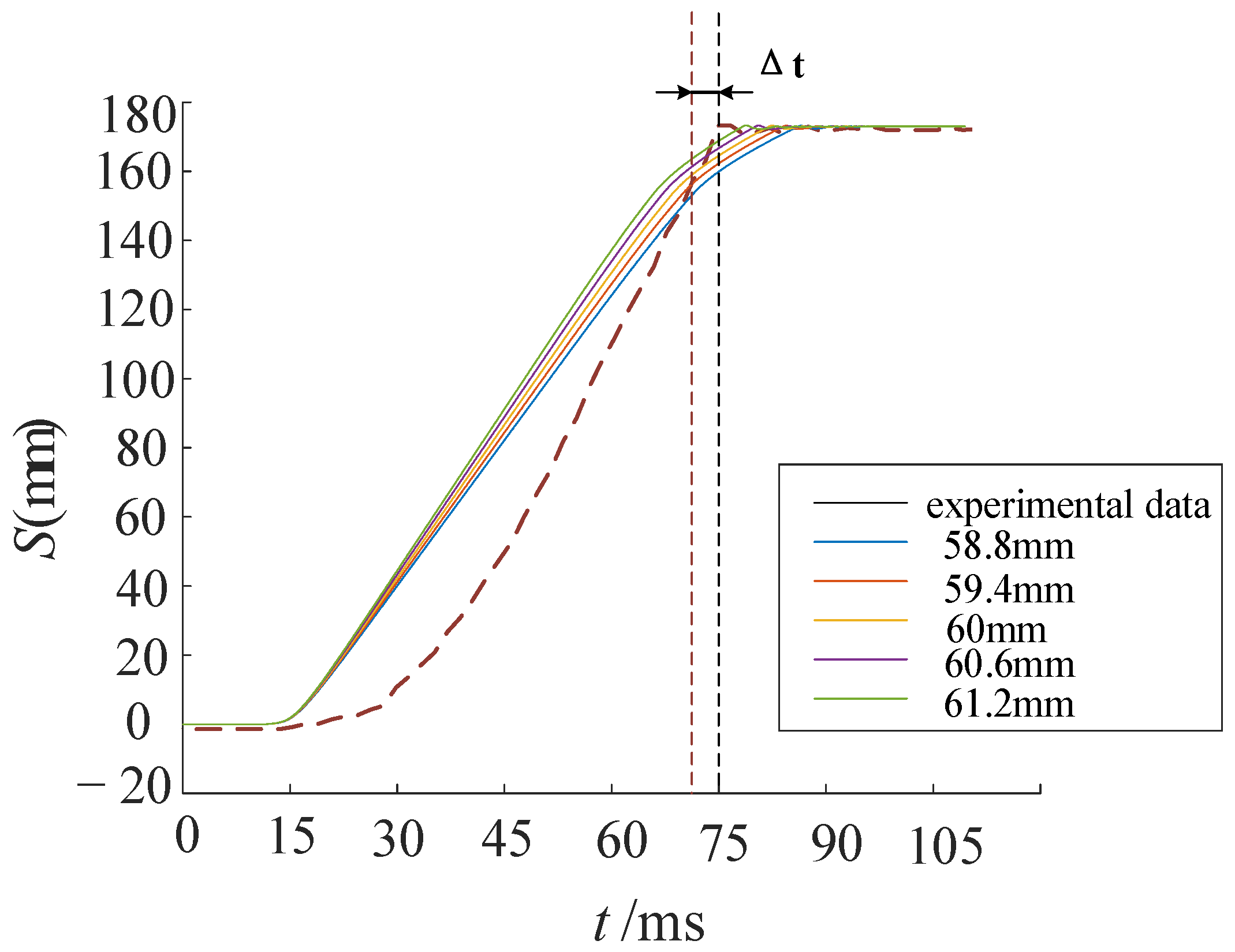
Figure 9 presents the test results from the mechanical property tester. The top pulse curve indicates the closing status, the middle curve represents the time-displacement stroke, and the bottom curve shows the solenoid valve current. The difference between the two vertical dashed lines on the left and right denotes the closing time. Figure 10 presents a comparison between simulation and experimental results. The colored solid lines represent the displacement of the working cylinder piston under different cylinder bore diameters. During the initial closing phase, the piston remains stationary with zero displacement. As high-pressure oil enters the rodless chamber of the working cylinder, the piston displacement increases due to differential pressure. As velocity gradually decreases, displacement changes stabilize. The figure shows that closing time decreases with increasing cylinder bore diameter. The red dashed line denotes the experimental curve, with a closing time difference of 1.6 ms (2.1% deviation) from the simulation curve, indicating good agreement. Discrepancies primarily arise from differences in leakage coefficients and fluid properties.
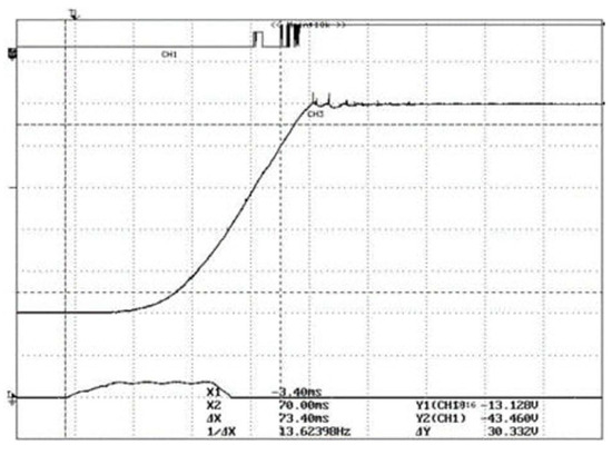
Figure 9.
Mechanical characteristic tester measurement results graph.
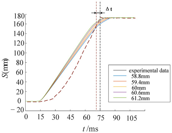
Figure 10.
Simulation and test results comparison.
2.5.2. Selection of Parameter Range
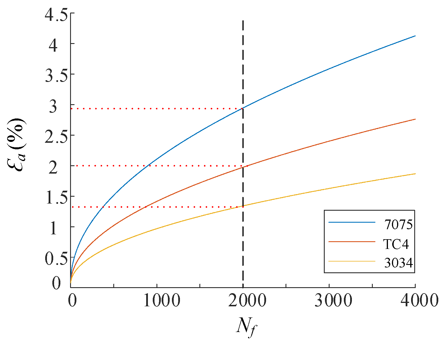
During the operation of the disc spring hydraulic operating mechanism in the circuit breaker, the working cylinder, main valve, and solenoid valve perform reciprocating linear motion. Due to the arc-extinguishing chamber’s switching, each component is subjected to asymmetric cyclic loads. As the number of operations increases, the fatigue damage to each component of the operating mechanism becomes more severe. The operating mechanism of the high-voltage circuit breaker experiences high stress due to the high-pressure oil and finite cyclic loading. In this low-cycle fatigue process, each switching action causes the material to undergo plastic deformation, resulting in a large strain amplitude, which leads to changes in the material’s microstructure and accumulated damage. To describe the variation process of each component under low-cycle fatigue conditions, the Coffin–Manson equation is used to model the relationship between the plastic deformation of each component and the number of cycles. This equation is applicable to the fatigue behavior of metallic materials under high stress and large strain conditions [32,33]:
where ɛa represents the strain amplitude; ɛ′f represents the fatigue ductility coefficient; b is the elastic region exponent; εf is the plastic region coefficient; c is the plastic region exponent; and Nf is the fatigue life.
Based on the actual materials used for the transmission components, the material properties, as shown in Table 3, are set for 7075 aluminum alloy, TC4 titanium alloy, and 304 stainless steel. The parameters for each material in the Coffin–Manson equation are presented in Table 4.
Table 3.
Main structural material parameters.
Table 4.
Material property.
The plastic strain amplitudes of the materials, corresponding to the pressure amplitude variations and material characteristics, are shown in Figure 11, based on the 2000-cycle requirement specified in the standard [34]. The deformation amplitudes for 7075, TC4, and 3034 were found to be 2.9%, 2%, and 1.4%, respectively.

Figure 11.
Typical operating conditions.
Based on this, the range of plastic strain amplitude variations caused by low-cycle fatigue in the structural components of the circuit breaker over its entire life cycle is determined, which in turn leads to the range of variation in the closing time of the high-voltage circuit breaker.
2.5.3. Working Cylinders
The parameter variation ranges for the working cylinder rod diameter, inner diameter, and piston stroke are ±2%, ±2%, and ±2.9%, respectively. The variation in the closing time of the high-voltage circuit breaker is shown in Figure 12. The blue color represents the difference value that exceeds the designed closing time, and the orange color represents the difference value that is less than the designed closing time. The same principle applies to Figure 13 and Figure 14 in the subsequent text.
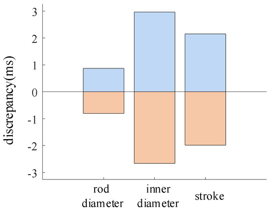
Figure 12.
The change in closing time under the change in working cylinder structure parameters.
During the operation of the circuit breaker, variations in the working cylinder rod diameter resulted in a closing time deviation of −0.8 ms to 0.87 ms. Variations in the inner diameter of the working cylinder led to a closing time deviation of −2.6 ms to 2.9 ms. Variations in the piston stroke of the working cylinder caused a closing time deviation of −1.9 ms to 2.1 ms.
2.5.4. Main Valve
The parameter variation ranges for the main valve rod diameter, inner diameter, and piston stroke are ±2.9%, ±2.9%, and ±2.9%, respectively. The variation in the closing time of the high-voltage circuit breaker is shown in Figure 13.
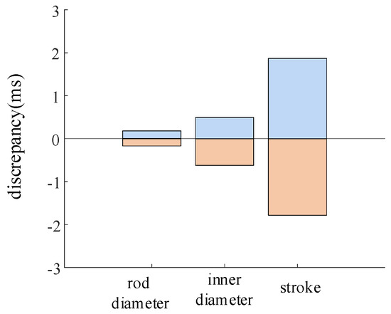
Figure 13.
The change in closing time under the change in main valve structure parameter.
Figure 13.
The change in closing time under the change in main valve structure parameter.
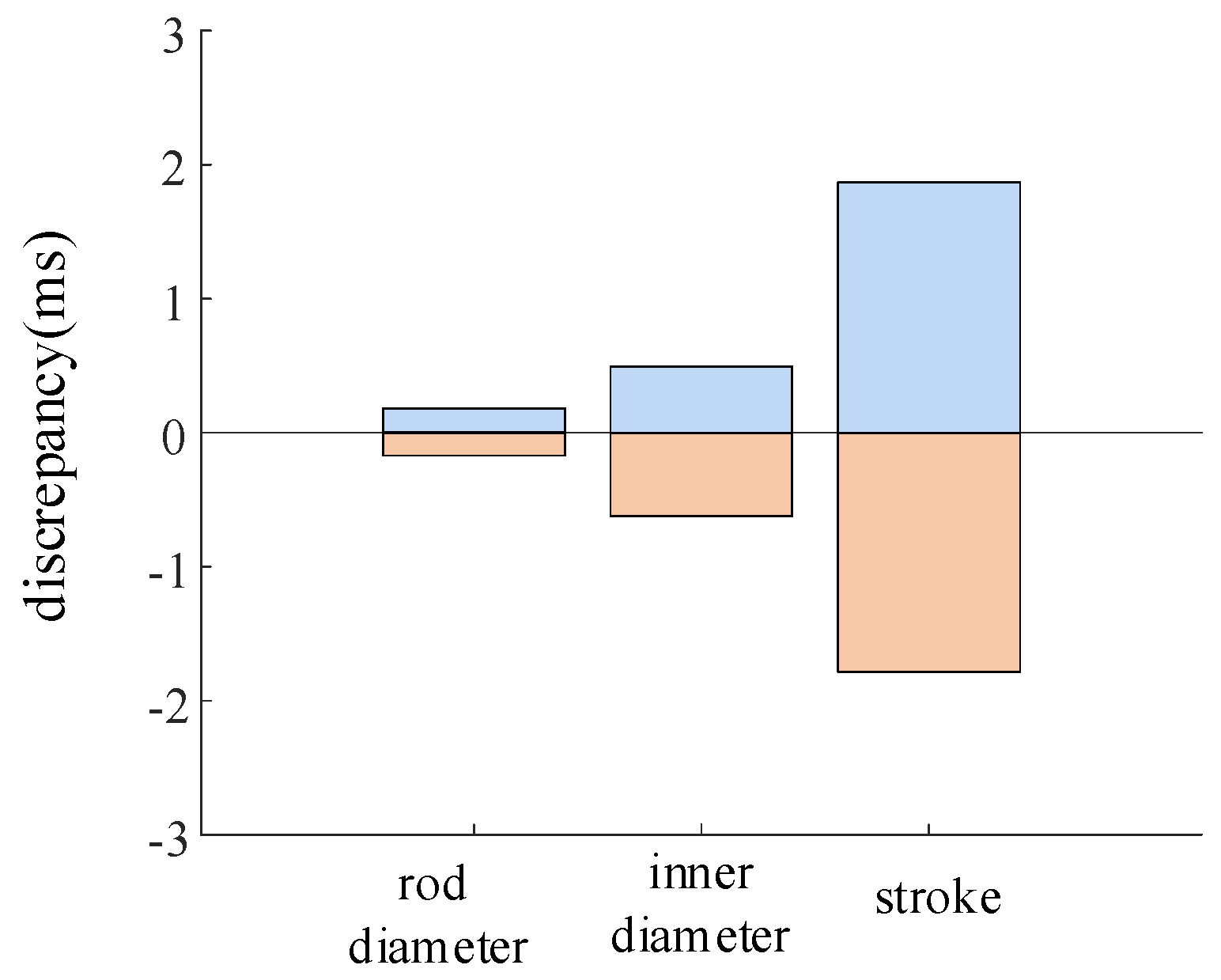
During the operation of the circuit breaker, variations in the main valve rod diameter resulted in a closing time deviation of −0.17 ms to 0.18 ms. Variations in the inner diameter of the main valve led to a closing time deviation of −0.62 ms to 0.49 ms. Variations in the stroke of the main valve caused a closing time deviation of −1.7 ms to 1.8 ms.
2.5.5. Solenoid Valves
The parameter variation ranges for the electromagnetic valve core diameter, valve seat hole diameter, and piston stroke are ±1.4%, ±1.4%, and ±1.4%, respectively. The variation in the closing time of the high-voltage circuit breaker is shown in Figure 14.
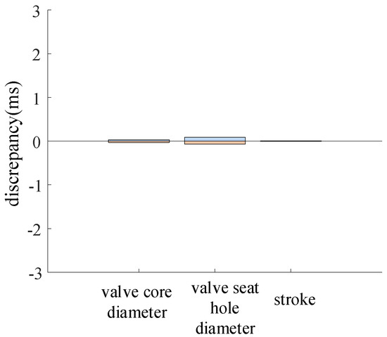
Figure 14.
The change in closing time under the change in solenoid valve parameters.
Figure 14.
The change in closing time under the change in solenoid valve parameters.
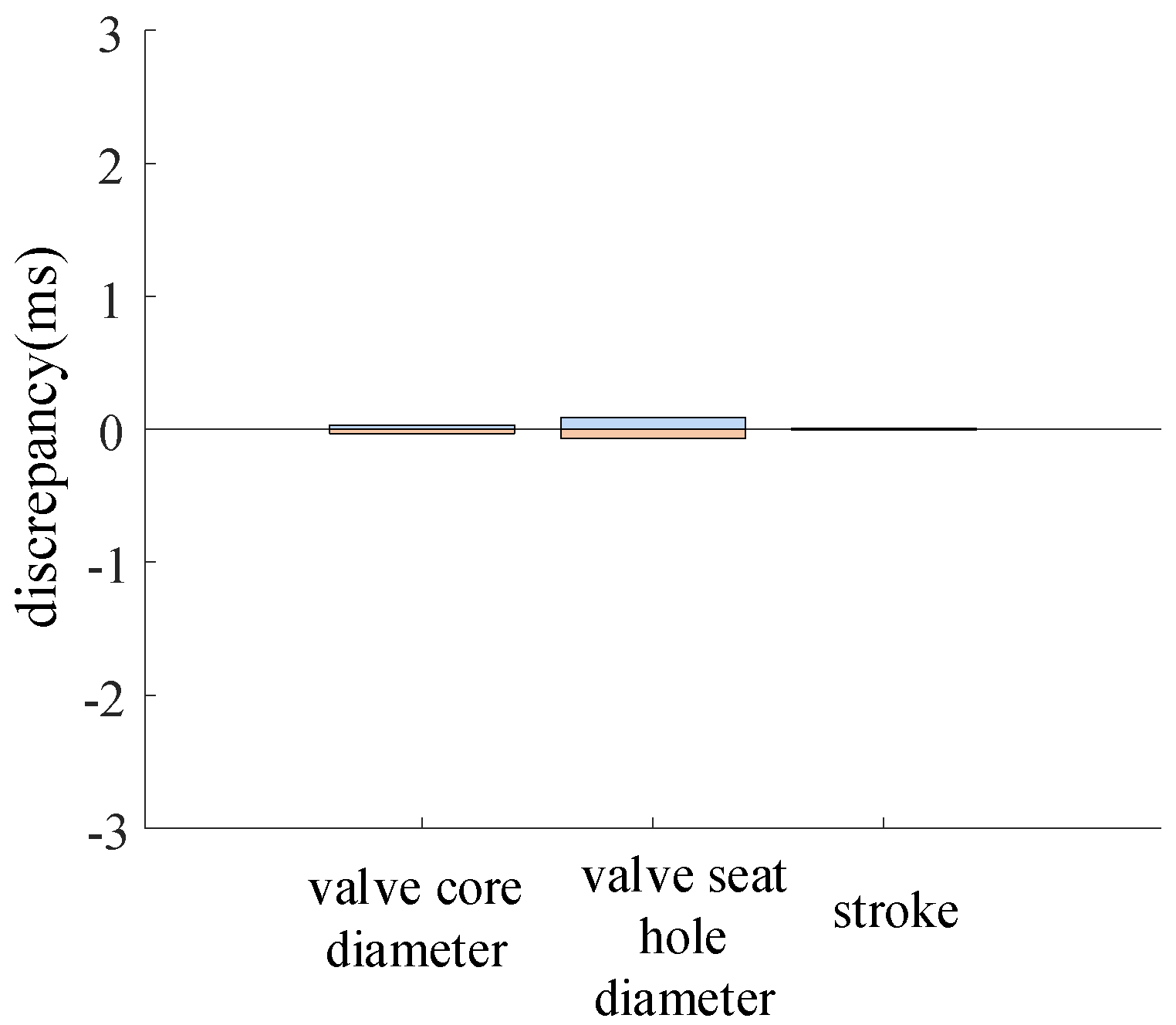
During the operation of the circuit breaker, variations in the electromagnetic valve resulted in an insignificant deviation in the closing time of the circuit breaker.
3. Reliability Analysis of Disc Spring Hydraulic Operating Mechanism
To quantitatively describe the impact of changes in the internal structure of the circuit breaker on the stability of the closing time, the influence weights under different mechanical dispersity requirements are analyzed. A stability analysis model needs to be established based on the simulation data of the closing time for the disc spring hydraulic operating mechanism.
3.1. Limit State Functions
In the closing process of the disc spring hydraulic operating mechanism, the closing time is a key indicator, which affects the accuracy of phase-controlled operations and the safe and stable operation of the power line. The closing time is defined as the time from when the circuit breaker receives the closing signal to when the contacts close, with the closing action being considered complete when the piston of the working cylinder reaches the rated stroke. In phase-controlled closing operations, the mechanical dispersity of the circuit breaker is defined as the difference between the actual action time and the rated action time. In reliability analysis, the system’s state is described by the limit state function g. The limit state function for the reliability of the operating mechanism’s closing time can be defined as the difference between the actual closing time and the rated closing time being less than the specified mechanical dispersity.
where Tσ = 3σ represents the specified mechanical dispersity; T(X) is the closing time during the fluctuation process of the circuit breaker’s structural parameters; X denotes the parameters; and Tμ is the rated action time of the circuit breaker.
3.2. Adaptive Kriging Surrogate Model
The key to the closing time stability of the disc spring hydraulic operating mechanism studied in this paper lies in estimating the structural failure probability, as shown in the following equation.
In the equation, denotes the distribution parameters of input variables, i.e., the dimensions of critical components in the operating mechanism; represents the distribution parameters of input variables; describes the uncertainties and probability density function of input variables, reflecting their stochastic sampling law; is the failure threshold, indicating that the system’s response does not meet the threshold requirement; and is the limit state function.
The numerical simulation method is a relatively general approach for estimating the failure probability. Based on the law of large numbers, this method uses the sample mean to estimate the population mean. That is, it transforms the integral for solving the failure probability in the above Formula (10) into the form of the mean. In other words, it estimates the failure probability using the frequency of failure. As long as there are a sufficient number of samples, the obtained estimated value will converge to the true failure probability. The most basic numerical simulation method is the Monte Carlo simulation method. This method first generates a set of samples of input variables according to the joint probability density function of the input variables. Then, it approximately estimates the failure probability through the ratio of the number of samples within the failure domain to the total number of samples. In contrast to the real and complex physical models, surrogate models have lower computational costs, so they can effectively improve the computational efficiency of the failure probability.
As an unbiased estimator with minimal estimation variance, the traditional Kriging surrogate model combines global approximation with local stochastic errors. Its effectiveness does not rely on the presence of random errors, and it demonstrates excellent fitting performance for highly nonlinear problems and local response discontinuities. Therefore, Kriging surrogate models can be employed to approximate both global and local function behaviors. The Kriging model can be expressed as the sum of a random distribution function and a polynomial [35,36]:
In the equation, is the unknown Kriging model; is the basis function of the random vector providing a global approximation model within the design space; are the regression coefficients to be determined, whose values can be estimated from known response values; p denotes the number of basis functions; is a stochastic process modeling local deviations with 0 mean and variance on top of the global approximation. The components of its covariance matrix can be expressed as follows:
In the equation, represents the correlation function between any two sample points, which serves as a component of the correlation matrix R, and m is the number of data points in the training sample set. Multiple functional forms are available for the , with the Gaussian correlation function expressed as
In the equation, represents the unknown correlation parameter. According to Kriging theory, the response estimate at an unknown point x is given by the following:
In the equation, is the estimate of , g is a column vector composed of response values from training samples, F is an dimensional matrix formed by regression models at m sample points, and is the correlation function vector between training samples and the prediction point, which can be expressed as follows:
In the equation, and variance estimate are given by the following:
The correlation parameter can be obtained by maximizing the likelihood function
The Kriging model constructed using the parameter obtained via maximum likelihood estimation is the surrogate model with optimal fitting accuracy.
Therefore, for any unknown follows a Gaussian distribution, , where the mean and variance are calculated as follows:
The Kriging surrogate model is an exact interpolation method. At training points , the model satisfies and . indicates the minimum mean squared error between and . The performance function values at initial sample points have zero error, while the variances of performance function predictions for other input variable samples are generally non-zero. When is large, it indicates that the estimate at point x is unreliable. Therefore, the predicted variance can be used to quantify the estimation accuracy of the surrogate model at location x, thereby providing an effective indicator for updating the Kriging surrogate model.
Traditional Kriging relies on fixed covariance functions and parameters, making it less adaptable to non-stationary data or dynamically changing environments. It cannot automatically update the model to accommodate new data, and parameters must be manually set, which may compromise results. In contrast, the adaptive Kriging model automatically optimizes covariance function parameters based on data characteristics, incorporates new data in real time, and updates the model dynamically.
The adaptive Kriging model is an improved spatial statistical model based on the traditional Kriging method. Its core idea is to enhance the fitting capability for complex data and prediction accuracy by dynamically adjusting model parameters or structures.
The framework for constructing an adaptive Kriging surrogate model is as follows: 1. Initial model construction: Build a coarse Kriging surrogate model using a small number of training samples. 2. Adaptive sampling: Select candidate samples that meet specified criteria from a pool of potential points via an adaptive learning function, and update the Kriging model iteratively until convergence criteria are satisfied. 3. Stability analysis: Conduct a stability analysis using the final updated Kriging surrogate model. Sample points added to the Kriging training set for model updating must satisfy two criteria: 1. They are located in regions with a high probability density of random input variables. 2. They are close to the failure surface where the performance function equals zero and where the risk of misclassifying the sign is high. Sample points with high risk of sign misclassification exhibit the following characteristics: 1. they are located near the limit state surface (i.e., small ); 2. they have high prediction variance from the current Kriging surrogate model; or 3. both conditions above simultaneously. The adaptive learning function selected here is the U-learning function [37].
The U-learning function considers both the distance of the Kriging surrogate model’s predicted value to the failure surface and the standard deviation of the estimate. Specifically, when predicted values are equal, larger standard deviations result in smaller U-learning function values; when standard deviations are equal, predicted values closer to zero yield smaller U-learning function values. Points near the failure surface with larger standard deviations of estimates should be added to the training dataset to update the Kriging model. Specifically, from the candidate sample pool, select the sample point with the smallest U-value and add this sample point along with its corresponding true performance function value to the training dataset to update the current Kriging model. Reference [37] indicates that using as the termination condition for the adaptive updating process of the Kriging surrogate model with the U-learning function is appropriate.
3.3. Directionally Important Sampling
For engineering problems involving extremely low failure probabilities under specific conditions, the Monte Carlo method requires a vast number of samples to achieve convergent results, leading to inefficient sampling. Therefore, improved mathematical modeling methods are proposed, with importance sampling being the most common approach. Importance sampling has gained extensive application due to its high sampling efficiency and small computational variance.
The basic concept of importance sampling is to replace the original sampling density function with an importance sampling density function, thereby increasing the probability of samples falling into the failure region and achieving higher sampling efficiency and faster convergence. The fundamental principle for selecting the importance sampling density function is to ensure that samples contributing significantly to the failure probability are sampled with higher probability, which reduces the variance of the estimate.
Compared to traditional Monte Carlo simulation in Cartesian coordinate systems, directional importance sampling offers superior efficiency and accuracy for failure probability problems involving a single limit state. By solving nonlinear equations instead of performing univariate random sampling, it reduces the dimension of the original random variable space to one.
The component dimensions of the hydraulic operating mechanism with disc springs are mutually independent normal variables. The directional sampling method analyzes structural stability through random sampling in the standard normal space under polar coordinates, utilizing the distribution properties of directional vectors . In the standard normal space, any random vector in Cartesian coordinates can be represented in polar coordinates as , where R is the polar radius and A is the unit directional vector of x. Under polar coordinates, the failure probability formula for the performance function can be expressed as follows:
In the equation, is the joint probability density function of the random vector x, is the joint probability density function of R and A. is the probability density function of the unit directional vector A. Since x follows an n-dimensional independent standard normal distribution, follows a uniform distribution on the unit sphere. is the conditional probability density function of the random variable R in the sampling direction A = a. defines the failure threshold when A = a, assuming the distance from the origin to the failure surface in the sampling direction A = a is r(a). The failure probability in the direction A = a can be obtained from the cumulative distribution function of a chi-squared distribution with n degrees of freedom, expressed as follows:
Thus, the unbiased estimator of structural failure probability and its variance are calculated as follows:
As an improved method of the directional sampling method, the basic idea of the directional importance sampling method is as follows: By establishing an important sampling density function to replace the original sampling density function, more sampling directions are directed towards the regions that make a greater contribution to the structural failure probability. This approach can improve the sampling efficiency and accelerate the convergence speed of the simulation process.
For the problem of failure probability in the limit state, the directional importance sampling method establishes an importance sampling density function in the polar coordinate system, and the failure probability is given by the following equation:
The directional importance sampling density function is given by the following:
In the equation, represents the stability index, is the indicator function, which equals 1 if and 0 otherwise. The control parameter p ranges within [0, 1]. When p = 1, the directional importance sampling density function degenerates into the directional sampling density function . When p = 0, directional importance sampling will only sample on one side of the failure domain of the limit plane. The closer the limit state surface approaches a planar surface, the closer the value of p can be chosen to 0; the closer the limit state surface approaches a spherical surface, the closer the value of p can be chosen to 1. The value of p can be appropriately selected between 0 and 1 to ensure that directional importance sampling effectively reflects the actual failure domain.
The unbiased estimate of the structural failure probability and the calculation formula for its variance are presented as follows:
3.4. Calculation Process
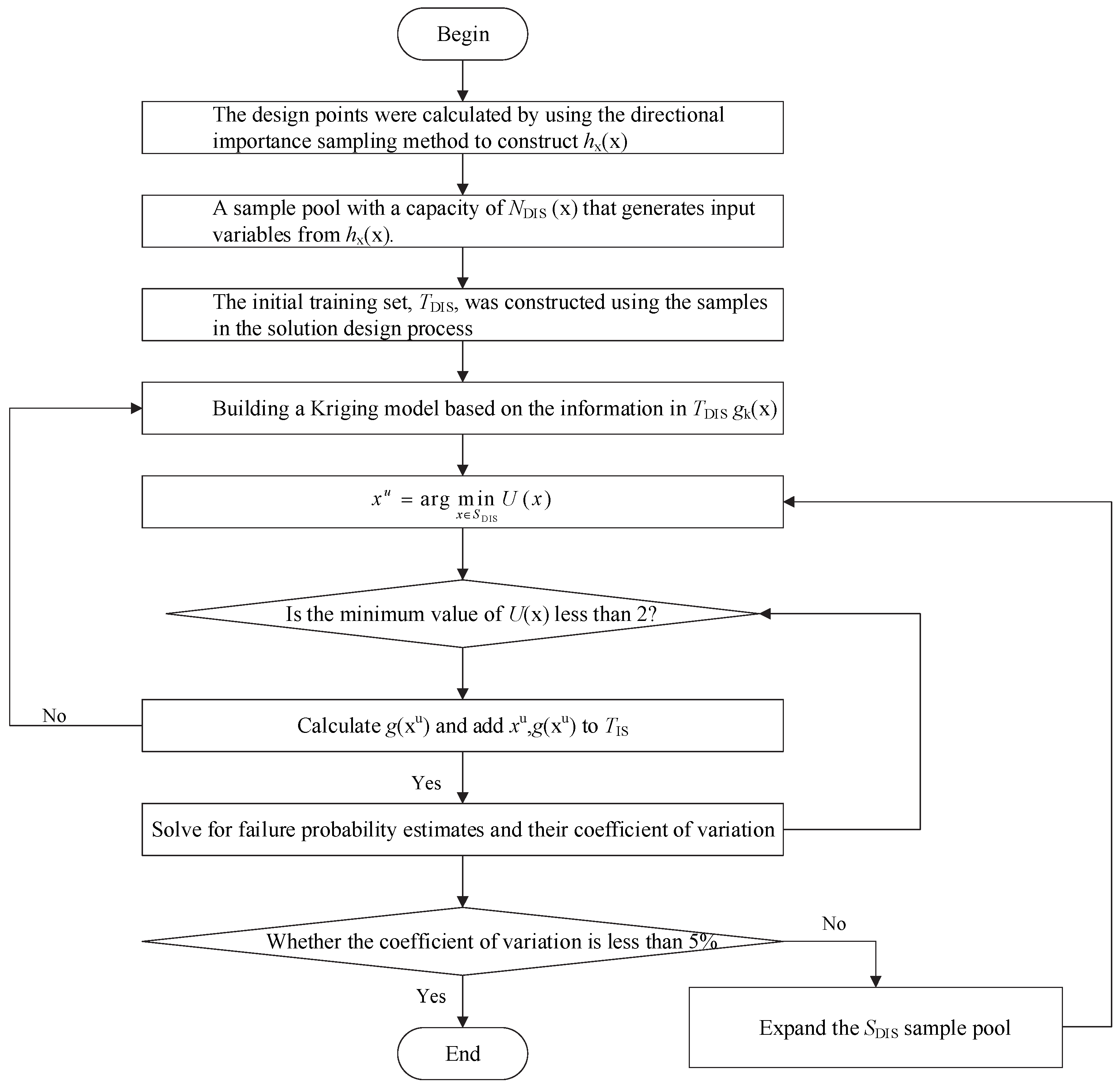
The main approach of the AK-DIS method for reliability analysis is as follows: First, the corresponding design point is obtained using the single-mode directional sampling method, and the sampling center of the original density function is shifted to the new design point. An importance sampling probability density function is constructed, and the single-mode sampling method is used to solve the input–output model data at the design point in order to build the original Kriging model. Next, the importance sampling density function is used to generate an importance sampling sample pool, and the U-learning function is employed to select the updated sample points that meet the requirements from the sample pool. The true function values are calculated for these points and added to the training sample set to iteratively update the Kriging model. Finally, the updated and converged Kriging model is used for reliability analysis. The process of solving reliability using the AK-DIS method is shown in Figure 15, with the specific calculation steps as follows:
- (1)
- The unimodal directional sampling density function is constructed by solving the design point P* using the unimodal directional method. The sampling center of the original sampling density function is shifted to P*, and the unimodal directional sampling density function hx(x) is constructed.
- (2)
- Construct a single-mode directional sampling sample pool and initial training set TIS: hx(x) is used to extract the sample pool SDIS with a sample size of NDIS, and the input–output samples in the process of solving the design points are used to form the initial training sample set TDIS.
- (3)
- Construct the Kriging model gk(x) based on the information in TDIS.
- (4)
- Select the update sample point xu in SDIS; then, there is the following:
- (5)
- Determine whether the self-learning process has converged: if the U-learning function is greater than 2, stop the adaptive learning process and proceed to step 6; otherwise, calculate g(xu), and add {xu, g(xu)} to the training samples in TDIS, and then return to step 3 to continue updating the Kriging model gk(x).
- (6)
- Use the current Kriging surrogate model to estimate the failure probability: use the Kriging surrogate model to calculate the failure domain indicator function value corresponding to each sample point in SDIS, and obtain the estimated value of the failure probability.
- (7)
- Calculate the coefficient of variation of the failure probability estimate to determine the convergence of AK-DIS reliability. When the coefficient of variation is less than 5%, the algorithm stops running.

Figure 15.
AK-DIS algorithm process.
Figure 15.
AK-DIS algorithm process.
4. Closing Time Prediction Model
By setting structural parameters to randomly vary 1000 times within the low-cycle fatigue deformation range, 9000 combinations of nine variables and corresponding data for switching time and variable values are obtained. These are then input into the AK-DIS reliability algorithm, with mechanical dispersion set at 3σ = ±1 ms, yielding global and local stability results. Monte Carlo Simulation (MCS) is employed to numerically simulate the simulation data and provide the exact solution. The Importance Sampling (IS) method and the Adaptive Kriging surrogate model combined with Monte Carlo Simulation (AK-MCS) are used for comparison. The reliability analysis results are shown in Table 5. In the table, Nd represents the number of real model calls, and n denotes the size of the alternative sample pool; Cov is the coefficient of variation.
Table 5.
Comparison of algorithm performance.
It can be observed that the failure probability estimates of the four methods are quite close, but the AK-DIS method exhibits the highest computational efficiency with the smallest error in failure probability Pf. From the perspective of a synchronized closing angle, when structural parameters experience low-cycle fatigue due to an increased number of actions, the failure probability is higher, making it difficult to meet the requirement within the mechanical dispersion of ±1 ms. In other words, the actual closing time of the high-voltage circuit breaker deviates significantly from the rated value.
To investigate the relationship between the accuracy and computational cost of the AK-DIS method, we analyzed the variations in computational time and accuracy by adjusting the candidate sample size as a proxy for computational cost, as shown in Figure 16. The results indicate that when the candidate sample pool ranges from 104 to 20 × 104, a better balance between accuracy and computational cost is achieved.
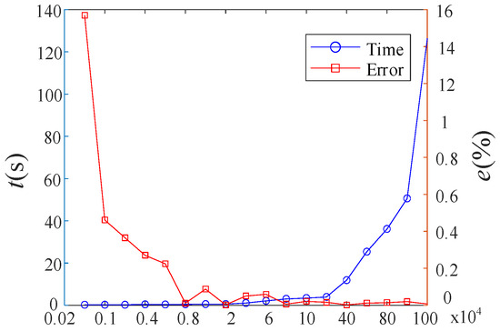
Figure 16.
Comparison of the Accuracy and Calculation Time of the AK-DIS Algorithm.
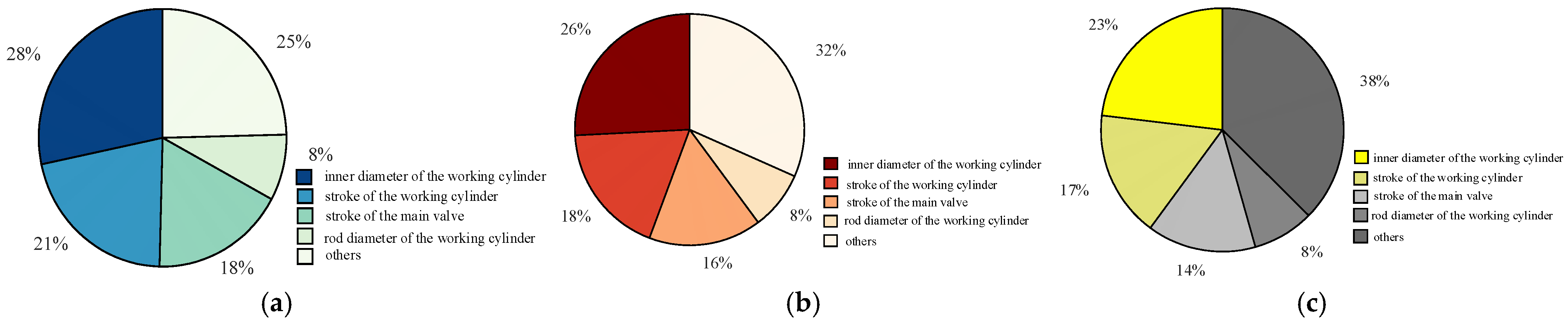
To facilitate the analysis of the influence weights of various parameters under different mechanical dispersions, the sensitivity is obtained by taking the partial derivative of the failure probability with respect to the mean value of each component. By comparing the sensitivity of individual variables with the sum of the sensitivities of all variables, the normalized stability impact weight of a single variable on the circuit breaker operation time is determined. Figure 17 illustrates the stability impact weights of parameters under different mechanical dispersions, while Figure 18 presents the stability impact weights of different parameters under different mechanical dispersion requirements.
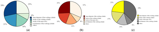
Figure 17.
Reliability influence weights of parameters under different mechanical dispersibility. (a) Mechanical dispersibility ± 1 ms. (b) Mechanical dispersibility ± 1.5 ms. (c) Mechanical dispersibility ± 2 ms.
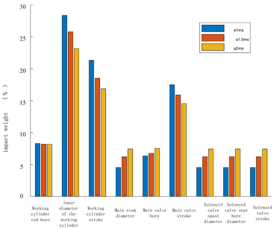
Figure 18.
The reliability influence weight changes of parameters under different mechanical dispersibility.
From Figure 17 and Figure 18, it can be observed that under different mechanical dispersion conditions, the degree of influence on the circuit breaker closing time, i.e., the parameters with a higher proportion of reliability impact weight on the circuit breaker, are listed in descending order as follows: working cylinder bore diameter, working cylinder stroke, main valve stroke, and working cylinder rod diameter, totaling four parameters. As the mechanical dispersion requirement gradually decreases, the proportion of the stability impact weight of these four variables also gradually decreases.
For switch manufacturers, in order to reduce the low-cycle fatigue caused by excessive opening and closing cycles, materials with high fatigue strength and good ductility should be selected. Stress concentration should be avoided, and all connection points should be designed reasonably. Optimizing the geometry can effectively disperse stress. Coatings or surface plating should be used to protect surfaces from corrosion, and regular inspections of critical components should be carried out to detect and repair early-stage damage in a timely manner.
Due to the compact structure of the disc spring hydraulic operating mechanism, which makes it difficult to disassemble and replace, a closing time prediction model is established based on the weight coefficients under different mechanical dispersions. The prediction results are compared with the no-load test results of the ultra-high voltage circuit breaker to verify the accuracy of the weight analysis. The closing time prediction model is shown in the following formula.
In the formula, T is the predicted closing time; is the weight coefficient of different components under different mechanical dispersions; is the life state of different components under different mechanical dispersions, that is, the ratio of the number of actuations to the total designed number of actuations; and is the closing time offset caused by the low-cycle fatigue of different components throughout their entire life cycle.
Since the components with a relatively large weight in the disc spring hydraulic operating mechanism are, respectively, the inner diameter of the working cylinder, the stroke of the working cylinder, the stroke of the main valve, and the diameter of the working cylinder rod, these four components are taken as the analysis basis for the closing time prediction model. The design of the no-load closing test is as follows: 250 no-load closing tests are carried out in the initial state after the circuit breaker leaves the factory. The closing time is recorded every 50 times to obtain five groups of data, so as to obtain the initial closing time of the operating mechanism. Then, 2000 closing tests are carried out, and the closing time is measured every 50 times to obtain 40 groups of data. Therefore, a total of 45 groups of data are obtained.
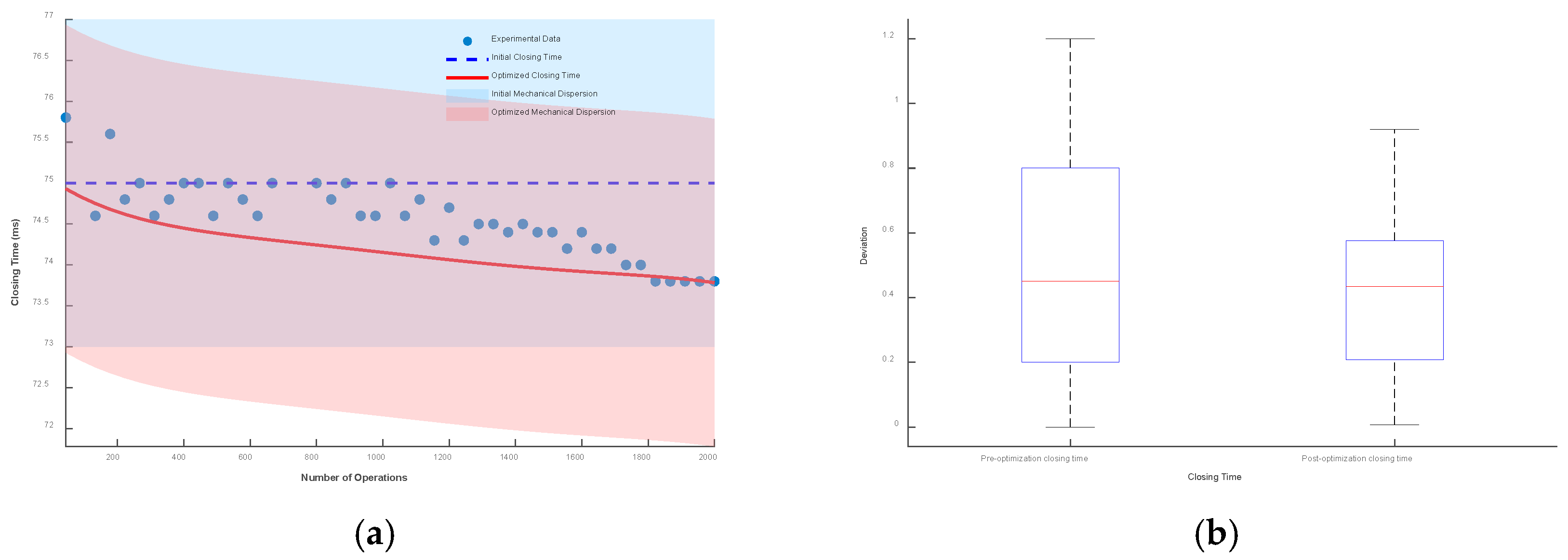
Taking the initial closing time as the reference, the envelope line composed of mechanical dispersion is drawn. Then, the closing time prediction model considering low-cycle fatigue is drawn, and the envelope line composed of its mechanical dispersion is also drawn. The results and box plots under different mechanical dispersions are shown in Figure 19, Figure 20 and Figure 21.
It can be seen from the figures that when the mechanical dispersion is ±1 ms, after the number of operations is greater than 1750 times, the actual closing time has exceeded the boundary of the initial mechanical dispersion, which seriously affects the control of the circuit breaker and the stability of the power system. When the mechanical dispersions are ±1.5 ms and ±2 ms, although the actual operating time will not exceed the set mechanical dispersion, the deviation between the optimized closing time prediction model and the actual operating time is smaller.
The box plot represents the deviation between the optimized closing time model, the unoptimized model, and the test data. Under the mechanical dispersions of ±1 ms, ±1.5 ms, and ±2 ms, the maximum deviation values of the optimized closing time prediction model are reduced by 12.8%, 20.4%, and 23.3%, respectively, and the fluctuation ranges are reduced by 37%, 38.3%, and 38.6%, respectively.
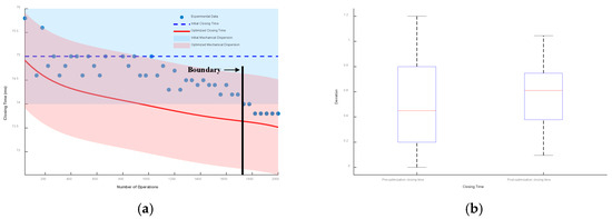
Figure 19.
Mechanical dispersion of ±1 ms: (a) deviation plot and (b) box plot.
Figure 19.
Mechanical dispersion of ±1 ms: (a) deviation plot and (b) box plot.
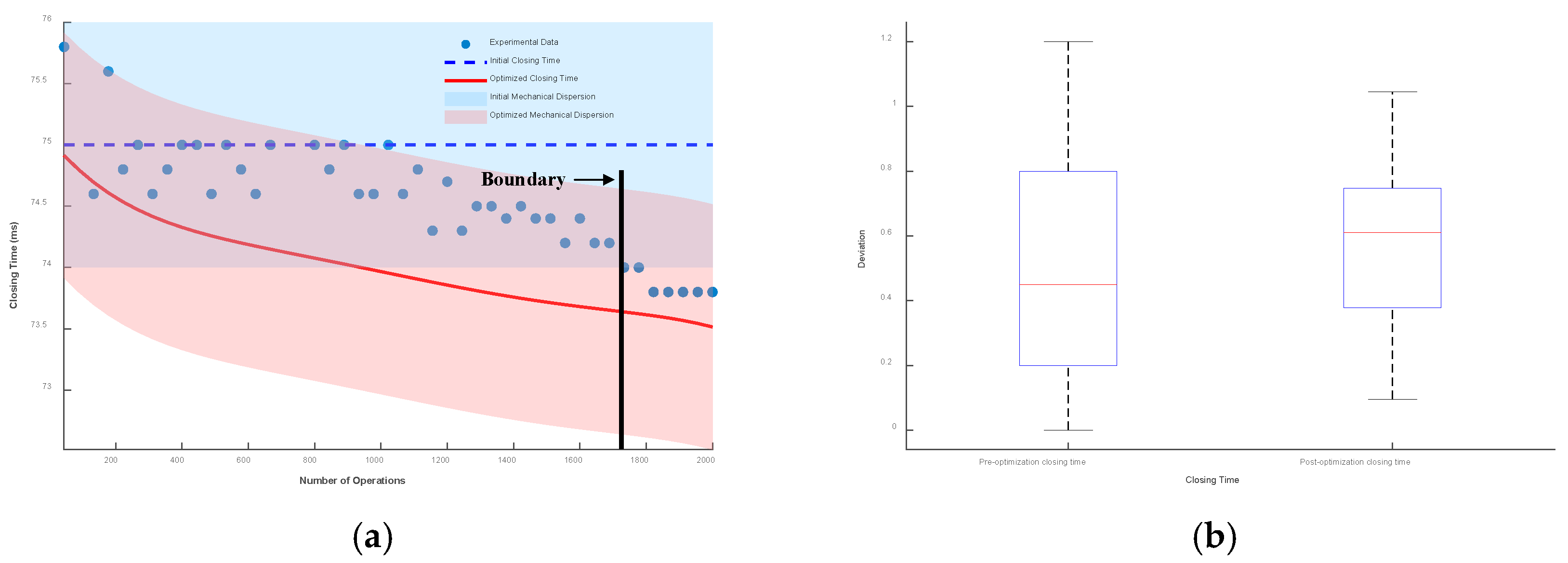

Figure 20.
Mechanical dispersion of ±1.5 ms: (a) deviation plot and (b) box plot.
Figure 20.
Mechanical dispersion of ±1.5 ms: (a) deviation plot and (b) box plot.
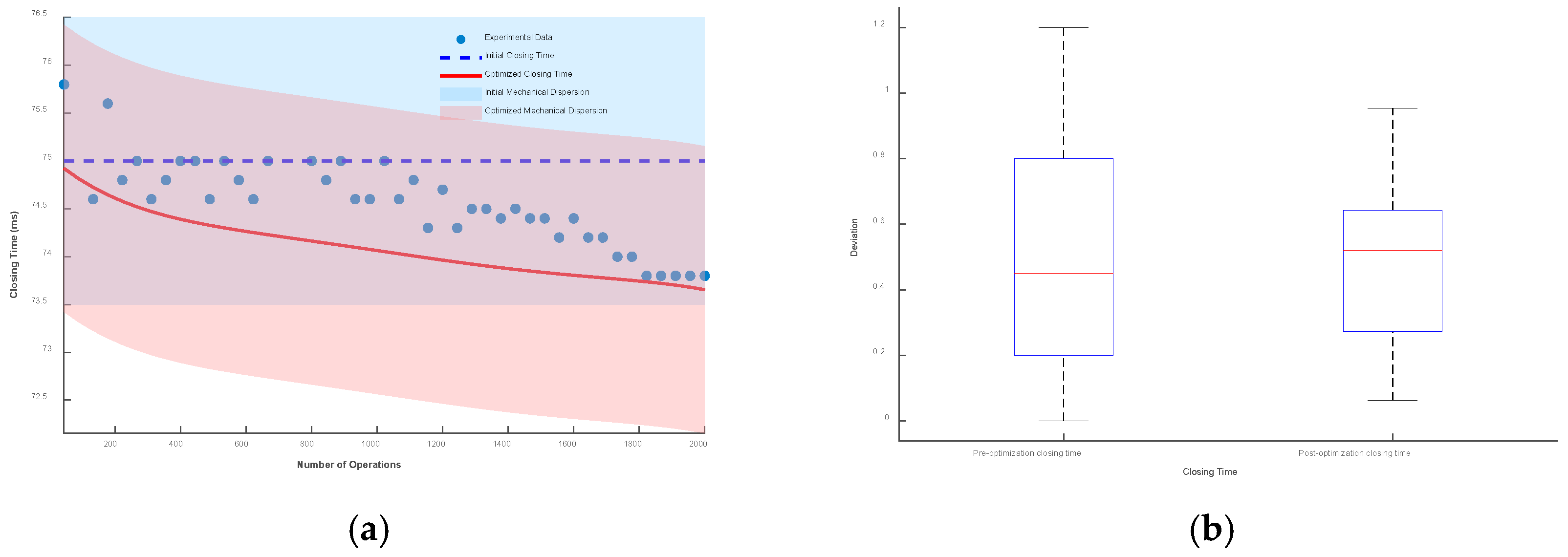

Figure 21.
Mechanical dispersion of ±2 ms: (a) deviation plot and (b) box plot.
Figure 21.
Mechanical dispersion of ±2 ms: (a) deviation plot and (b) box plot.
5. Conclusions
To design a closing time prediction model for ultra-high-voltage disc spring hydraulic operating mechanism circuit breakers considering low-cycle fatigue, a closing transmission chain simulation model was first developed to analyze the dynamic characteristics of circuit breakers under low-cycle fatigue. Then, the AK-DIS algorithm was constructed to analyze the influence weights of dimensional variations of components on closing time stability. Finally, a closing time prediction model was designed based on dynamic weight changes, significantly improving prediction accuracy.
- (1)
- By analyzing the transmission process of the circuit breaker operating mechanism, the deformation ranges of working components caused by low-cycle fatigue were calculated and substituted into the model simulation. The resulting fluctuation range of the circuit breaker’s operating time was −2.6 ms to 2.9 ms, significantly exceeding the mechanical dispersion requirements.
- (2)
- By processing the stability analysis results, the influence degrees of different parameters on closing time stability under various mechanical dispersions were obtained. Among them, four parameters—working cylinder inner diameter, working cylinder stroke, main valve stroke, and working cylinder rod diameter—each accounted for more than 10% under any mechanical dispersion.
- (3)
- A closing time prediction model considering the low-cycle fatigue of the operating mechanism was designed. Through comparison with no-load closing tests, under mechanical dispersions of ±1 ms, ±1.5 ms, and ±2 ms, the maximum deviation values of the optimized model were reduced by 12.8%, 20.4%, and 23.3%, respectively, while the fluctuation ranges were reduced by 37%, 38.3%, and 38.6%, respectively.
Author Contributions
Conceptualization, Q.L.; Methodology, X.Y.; Software, K.J.; Validation, M.H. and X.D.; Formal analysis, M.L.; Investigation, W.L.; Resources, X.P. and D.H.; Writing—original draft, D.X. All authors have read and agreed to the published version of the manuscript.
Funding
This research was funded by Science and Technology Project of China Southern Power Grid grant number CGYKJXM20220346 and The APC was funded by China Southern Power Grid.
Data Availability Statement
The original contributions presented in this study are included in the article. Further inquiries can be directed to the corresponding author.
Conflicts of Interest
Authors Qi Long, Xu Yang, Keru Jiang, Weiguo Li, Mingyang Li, Mingchun Hou, Xiang Peng and Dachao Huang were employed by the company EHV Power Transmission Company China Southern Power Grid. The remaining authors declare that the research was conducted in the absence of any commercial or financial relationships that could be construed as a potential conflict of interest.
References
- Maller, V.N.; Naigu, M.S. Advances in High Voltage Insulation and Arc Interruption in SF6 and Vacuum; Pergamon: Oxford, UK, 1981; pp. 100–118. [Google Scholar]
- Nakanishi, K. Switching Phenomena in High-Voltage Circuit Breakers; Marcel Dekker: New York, NY, USA, 1991; pp. 102–104. [Google Scholar]
- Garzon, R.D. High Voltage Circuit Breakers: Design and Applications, 2nd ed.; Marcel Dekker: New York, NY, USA, 2002; pp. 212–216. [Google Scholar]
- Huang, Y.; Wang, J.; Zhang, W.; Al-Dweikat, M.; Li, D.; Yang, T.; Shao, S. A motor-drive-based operating mechanism for high-voltage circuit breaker. IEEE Trans. Power Deliv. 2013, 28, 2602–2609. [Google Scholar] [CrossRef]
- Liu, W.; Xu, B.; Yang, H.; Zhao, H.; Wu, J. Hydraulic operating mechanisms for high voltage circuit breakers: Progress evolution and future trends. Sci. China Technol. Sci. 2011, 54, 116–125. [Google Scholar] [CrossRef]
- Wang, F.; Gu, L.Y.; Chen, Y. A hydraulic pressure-boost system based on high-speed on–off valves. IEEE/ASME Trans. Mechatron. 2012, 18, 733–743. [Google Scholar] [CrossRef]
- Yao, J.; Jiao, Z.; Ma, D.; Yan, L. High-Accuracy tracking control of hydraulic rotary actuators with modeling uncertainties. IEEE/ASME Trans. Mechatron. 2013, 19, 633–641. [Google Scholar] [CrossRef]
- Wang, F.; Chen, Y. Dynamic characteristics of pressure compensator in underwater hydraulic system. IEEE/ASME Trans. Mechatron. 2013, 19, 777–787. [Google Scholar] [CrossRef]
- Cano-González, R.; Bachiller-Soler, A.; Rosendo-Macías, J.A.; Álvarez-Cordero, G. Controlled switching strategies for transformer inrush current reduction: A comparative study. Electr. Power Syst. Res. 2017, 145, 12–18. [Google Scholar] [CrossRef]
- Parikh, U.B.; Bhalja, B.R. Mitigation of magnetic inrush current during controlled energization of coupled un-loaded power transformers in presence of residual flux without load side voltage measurements. Int. J. Electr. Power Energy Syst. 2016, 76, 156–164. [Google Scholar] [CrossRef]
- Chandrasena, W.; Jacobson, D.; Wang, P. Controlled switching of a 1200MVA transformer in Manitoba. IEEE Trans. Power Deliv. 2016, 31, 2390–2400. [Google Scholar] [CrossRef]
- Elvis, B.; Adam, M.; Andruşcă, M.; Micu, M. Aspects regarding the controlled switching of the shunt reactors. In Proceedings of the 2016 International Conference and Exposition on Electrical and Power Engineering (EPE), Iasi, Romania, 20–22 October 2016; pp. 119–122. [Google Scholar]
- Stanek, M. Analysis of circuit breaker controlled switching operations—From manual to automatic. In Proceedings of the 2015 50th International Universities Power Engineering Conference (UPEC), Trent, UK, 1–4 September 2015; pp. 1–6. [Google Scholar]
- Duan, X.Y.; Huang, Z.H.; Liao, M.F.; Ding, F.H. Prediction and compensation of operating time based on multi-element linear regression for controlled switching. Electr. Power Autom. Equip. 2009, 29, 72–75. [Google Scholar]
- Bai, S.Y.; Wei, J.C.; Sun, S.P. Research on the synchronous closing controlof an intelligent breaker. J. Xihua Univ. Nat. Sci. 2009, 28, 17–20. [Google Scholar]
- Fangang, M.; Shijing, W.; Jicai, H.; Yang, X.; Junfeng, J.; Qiaoquan, L.; Cunling, S. Simulation and stability analysis of spring operating mechanism with clearance for high voltage circuit breakers. In Proceedings of the 2016 China International Conference on Electricity Distribution (CICED), Xi’an, China, 10–13 August 2016; pp. 1–5. [Google Scholar]
- Zhao, W.; Dang, D.; Di, Z.; Liu, C. Optimal Design and Fatigue Life Analysis on Buffer in Spring Mechanism. High Volt. Appar. 2017, 53, 6. [Google Scholar]
- Liu, Y.; Zhang, G.; Zhao, C.; Lei, S.; Qin, H.; Yang, J. Mechanical Condition Identification and Prediction of Spring Operating Mechanism of High Voltage Circuit Breaker. IEEE Access 2020, 8, 210328–210338. [Google Scholar] [CrossRef]
- Xu, B.; Ding, R.; Zhang, J.; Sha, L.; Cheng, M. Multiphysics-Coupled Modeling: Simulation of the Hydraulic-Operating Mechanism for a SF6 High-Voltage Circuit Breaker. IEEE/ASME Trans. Mechatron. 2016, 21, 379–393. [Google Scholar] [CrossRef]
- Gonzalez, J.J.; Freton, P. Flow behavior in high-voltage circuit breaker. IEEE Trans. Plasma Sci. 2011, 39, 2856–2857. [Google Scholar] [CrossRef]
- Pinto, L.C.; Zanetta, L.C. Medium voltage SF6 circuit-breaker arc model application. Electr. Power Syst. Res. 2000, 53, 67–71. [Google Scholar] [CrossRef]
- Looe, H.M.; Brazier, K.J.; Huang, Y.; Coventry, P.F.; Jones, G.R. High frequency effects in SF6 circuit breakers. IEEE Trans. Power Deliv. 2004, 19, 1095–1104. [Google Scholar] [CrossRef]
- Mori, T.; Kawano, H.; Iwamoto, K.; Tanaka, Y.; Kaneko, E. Gas-flow simulation with contact moving in GCB considering high-pressure and high-temperature transport properties of SF6 gas. IEEE Trans. Power Deliv. 2005, 20, 2466–2472. [Google Scholar] [CrossRef]
- Ding, F. Research on High Voltage Circuit Breaker with Hydraulic Operating Mechanism; Zhejiang University Hangzhou: Zhejiang, China, 1994; pp. 4–30. (In Chinese) [Google Scholar]
- Bošnjak, S.; Petković, Z.; Zrnić, N.; Pantelić, M.; Obradović, A. Failure analysis and redesign of the bucket wheel excavator two-wheel bogie. Eng. Fail. Anal. 2010, 17, 473–485. [Google Scholar] [CrossRef]
- Arsić, M.; Bošnjak, S.; Gnjatović, N.; Sedmak, S.A.; Arsić, D.; Savić, Z. Determination of residual fatigue life of welded structures at bucket-wheel excavators through the use of fracture mechanics. Procedia Struct. Integr. 2018, 13, 79–84. [Google Scholar] [CrossRef]
- Liu, W.; Zeng, Q.; Qin, W.; Wan, L.; Liu, J. Lifetime reliability of hydraulic excavators’ actuator. IEEE Access 2023, 11, 117670–117684. [Google Scholar] [CrossRef]
- Mohammad, J.; Odinokova, I.; Gaevskiy, V.; Nosko, E. Optimization design of the stick of an excavator under uncertain loading (in the conditions of the Syrian Arab Republic). MATEC Web Conf. 2021, 341, 00014. [Google Scholar] [CrossRef]
- Ma, T.; Gu, J.; Duan, M. Dynamic response of pipes conveying two-phase flow based on Timoshenko beam model. Mar. Syst. Ocean Technol. 2017, 12, 196–209. [Google Scholar] [CrossRef]
- Wei, Y.; Deng, G.; Yang, Z. Experimental study and numerical analysis of fluid-structure coupling vibration characteristics for the reciprocating compressor pipeline. IOP Conf. Ser. Earth Environ. Sci. 2020, 558, 022007. [Google Scholar]
- Fan, S.; Xu, R.; Ji, H.; Yang, S.; Yuan, Q. Experimental Investigation on Contaminated Friction of Hydraulic Spool Valve. Appl. Sci. 2019, 9, 5230. [Google Scholar] [CrossRef]
- Huang, J.; Shi, D.; Yang, X.; Yu, H.; Dong, C. Unified modeling of high temperature deformations of a Ni-based polycrystalline wrought superalloy under tension-compression, cyclic, creep and creep-fatigue loadings. Sci. China Technol. Sci. 2015, 58, 248–257. [Google Scholar] [CrossRef]
- Ambroziak, A. Application of elasto-viscoplastic Bodner-Partom constitutive equations in finite element analysis. Comput. Assist. Methods Eng. Sci. 2022, 14, 405–429. [Google Scholar]
- GB/T 30846-2014; High-Voltage Alternating Current Circuit-Breakers with Intentionally Non-Simultaneous Pole Operation. General Administration of Quality Supervision, Inspection and Quarantine of the People’s Republic of China, Standardization Administration of the People’s Republic of China: Beijing, China, 2014.
- Echard, B.; Gayton, N.; Lemaire, M.; Relun, N. A combined im-portance sampling and Kriging reliability method for small fail-ure probabilities with time demanding numerical model. Reliab. Eng. Syst. Saf. 2013, 111, 232–240. [Google Scholar] [CrossRef]
- Rausand, M.; Hoyland, A. System Reliability Theory: Models, Statistical Methods, and Applications; John Wiley & Sons Inc.: Hoboken, NJ, USA, 2020. [Google Scholar]
- Echard, B.; Gayton, N.; Lemaire, M. AK—MCS: An active learning reliability method combining Kriging and Monte Carlo Simulation. Struct. Saf. 2011, 33, 145–154. [Google Scholar] [CrossRef]


Disclaimer/Publisher’s Note: The statements, opinions and data contained in all publications are solely those of the individual author(s) and contributor(s) and not of MDPI and/or the editor(s). MDPI and/or the editor(s) disclaim responsibility for any injury to people or property resulting from any ideas, methods, instructions or products referred to in the content. |
© 2025 by the authors. Licensee MDPI, Basel, Switzerland. This article is an open access article distributed under the terms and conditions of the Creative Commons Attribution (CC BY) license (https://creativecommons.org/licenses/by/4.0/).