Abstract
The digital transformation of manufacturing requires an accurate measurement and analysis of process parameters to optimize efficiency, quality and cost control. This paper introduces a structured sensor selection cycle, providing a systematic approach for identifying relevant metrics, evaluating sensor technologies and integrating them into existing production systems. The proposed methodology enables companies to enhance process transparency, leading to data-driven decision-making and more flexible production strategies. Developed within the ZuPro2Flex research project, this framework offers practical guidance for aligning sensor technology with business model requirements.
1. Introduction
Collecting and analyzing process data are a key challenge in modern production environments. In order to ensure accurate and transparent process monitoring, the selection of suitable sensor technology is crucial. This guide was developed as part of the ZuPro2Flex research project funded by the German Federal Ministry of Education and Research. ZuPro2Flex [1] (title of the research project: “Condition assessment and process assistance for service life-based business models for increasing flexibility in production”) develops methods and concepts for utilizing pay-per-X business models to enhance production flexibility. It integrates machine-specific usage indices, process assistance and digital security mechanisms. Pay-per-X business models, which are flexible pricing strategies where customers pay based on actual usage, performance or achieved outcomes rather than a fixed purchase price, play a key role in this approach. Examples such as pay-per-use, pay-per-output and pay-per-performance are already widely applied in industries like machinery, software and services. By leveraging these models, ZuPro2Flex enables more adaptive and economically viable production strategies. One of the aims of this research project was to provide companies with a structured procedure for identifying, evaluating and implementing sensors for process transparency. Both the technical and economic aspects of sensor selection are considered. This guide is particularly aimed at users wishing to implement pay-per-x business models, where the accurate measurement of process parameters is essential for billing and quality assurance.
2. User Guide for Process Transparency
The basic prerequisite for pay-per-x business models is that the process parameters relevant to billing are known and can be determined. These can be parameters such as production figures, movements of the machine components, volume flows, time, etc.
It is necessary to define process windows in the pay-per-x business model to take into account the load on the processes. These windows, which include parameters such as forces, strains, temperatures and speeds, need to be monitored to ensure that the machines and components are operating within acceptable limits. The aim is to develop and validate a methodology to determine appropriate process windows in line with the business model to prevent excessive stress and wear.
The main objective is to develop a methodology that can be used to evaluate existing sensors and identify missing sensors. These sensors will be used to evaluate and monitor the processes that are critical to the pilot companies’ intended business models. Once identified, the missing sensors will be integrated into the existing system.
This user guide will present a general procedure for determining process transparency and selecting sensors. For all further and more in-depth questions on the selection process for sensors for process transparency, please refer to Section 3 of this text. There, a general concept for sensor selection and an application example from practice are presented.
2.1. The Three Pillars of the Pay-per-X Business Model
Before discussing process transparency at this point, there are a few considerations necessary for a general understanding of how the pay-per-x business model works.
Invoicing for this business model is based on the so-called “three pillars of pay-per-x” (Figure 1), namely the following:
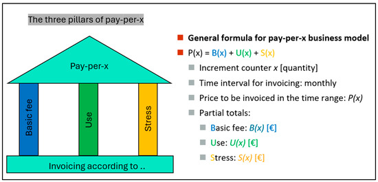
Figure 1.
The three pillars of the pay-per-x business model (blue: Basic fee B(x); green: Use U(x); yellow: Stress S(x)).
- Basic fee;
- Use: The use of the machine or component;
- Stress.
The general formula of the pay-per-x business model is as follows:
P(x) = B(x) + U(x) + S(x)
The expression P(x) represents the price to be billed for usage in the agreed time range—usually monthly. This expression is made up of the partial sums of the following:
- the monthly basic fee B(x);
- the use U(x) of the machine or component;
- the stress S(x)—this means the intensity of the usage behavior.
The x is the increment counter of usually one or more billing-relevant parameters. The expression U(x) stands for billing according to usage, which can be determined by various parameters, e.g.,
- operating time;
- power consumption;
- pieces produced;
- length produced, etc.
These parameters, which represent usage, are the so-called billing increments—i.e., the aforementioned billing-relevant parameters—and are the subject of this guide in the context of process transparency and its determination.
The term S(x) stands for billing according to stress, where the usage alone is not only decisive for billing but also the actual stress of the production machine. Additional amounts can be invoiced for disproportionate utilization. This includes utilization in the form of the following:
- wear (e.g., mechanical abrasion);
- material fatigue;
- ageing, etc.
These parameters, for which the stress must be determined by measurement, belong to the area of so-called condition transparency, rather than process transparency. Often, condition transparency is not yet known during the previous usage process of the machine or component. Instead, it requires prior investigations in order to identify comprehensible stress increments. The stress must be determined qualitatively (at what point is a stress “excessive”?) and then the excessive stress must be determined quantitatively (what amount of money serves as compensation for an “excessive” intensity of use?). Condition transparency and its determination are not part of this guide.
The term B(x) stands for a fixed monthly basic fee that serves as a guarantee of minimum usage or minimum income and is intended to prevent a loss scenario for the provider (the lessor of the machine or component).
This conceptual structure is consistent with current research into the transformation of ownership-based into usage-based business models. In particular, it reflects the three-part pricing logic proposed for complex manufacturing systems, which emphasizes basic availability, actual use and load-induced wear as key cost drivers. A methodical approach for implementing such models—especially under conditions of high system complexity and technological customization—is outlined in [2].
2.2. Definitions of Terms
The most important terms for the user guide are briefly defined below:
- Process transparency: Parameters that characterize the use of the respective system, machine or components and monitor their compliance (as previously agreed; protection against overload) or must be taken into account in billing (high load = higher costs). The parameters that characterize usage reflect the creation of added value and legitimize the counting of billing increments to form the monthly billing amount.
- Condition transparency: Parameters that are necessary to determine the current wear condition and wear progress of the respective system, machine or component.
- Billing basis: Parameters required for billing pay-per-x business models (e.g., operating hours, number of parts produced, number of strokes, etc.).
- Billing-relevant parameters: Billing increments record the scope of use and form the billing basis for the scope of the service used. Usage increments record the intensity of usage behavior and form the billing basis for the deterioration of the target status of the application.
- Extended service: Parameters that are required for the provision of additional services (in addition to pay-per-x).
To emphasize once again at this point, the term process transparency should be used to determine the parameters for usage and consequently also the load on the machine/component, which then form the scope of usage and the basis for billing in the form of billing increments. However, the qualitative and quantitative determination of “load” in the sense of wear, deterioration of the machine, etc., does not belong to process transparency, but to condition transparency. This is an important distinction between terms that many people interested in the pay-per-x business model for the first time cannot clearly separate.
However, this user guide for process transparency cannot do without taking into account the deterioration of the target state of the application: even if a machine manufacturer (the lessor of the machine or component) offers their machines for the first time in the pay-per-x business model and does not have a sufficient knowledge base for condition transparency, they can define certain process windows based on previous findings and knowledge, within which the machine may be operated and to which the machine user must adhere. Otherwise, exceeding these process windows must lead to additional payments or even to the machine being taken out of service. The machine manufacturer should at least know the interdependencies when these process windows are exceeded and communicate them to the user. In the long term, determining condition transparency could be advantageous for the design of the business model, but in the medium term, the machine manufacturer should at least know the process windows in order to counteract the deterioration of the target status of the application and be financially compensated for excessive stress.
2.3. Comparison of Pay-per-X Model vs. Investment Model in the Automotive Supply Industry
A project partner within the ZuPro2Flex research project from the automotive supplier industry provided a press hardening system for a comprehensive process and cost analysis. Their aim was to examine the cost structure of press hardening in detail and to compare alternative financing models—in particular a pay-per-X model—with the classic investment model.
The analysis was carried out in 2021, and accordingly, all calculations are based on the prices and framework conditions valid at that time.
2.3.1. Process Overview
Press hardening is a manufacturing process used in the automotive industry to produce ultra-high-strength steel components. The process comprises the following main steps:
- Heating phase (furnace with natural gas)
- The raw sheets are heated in a high-temperature furnace.
- The furnace is operated with natural gas and reaches an austenitising temperature of approx. 950 °C.
- The gas consumption varies depending on the material thickness.
- Transport and positioning (robotics)
- A robot removes the heated sheet and positions it in the press.
- Timing is crucial to minimize heat loss.
- Forming and quenching (press operation and tool cooling)
- The sheet is pressed into the final shape and simultaneously cooled quickly by an integrated water cooling system.
- This martensitic transformation significantly increases the strength.
- The press requires electrical energy, and the cooling system consumes water and additional energy for heat dissipation.
- Finishing (cutting, inspection and transportation)
- The hardened component is cut to size, checked for dimensional accuracy and prepared for further processing.
Each of these steps consumes specific resources (energy, gas, water, compressed air and machine wear), which must be recorded for a pay-per-X pricing model. The aim is to present the costs per production unit transparently.
2.3.2. Pay-per-X Cost Model with Basic Fee
The pay-per-X model is an alternative financing and usage method for production equipment in which a usage-based payment is made instead of a separate investment. In order to secure a calculable source of income for the machine rental company, a fixed monthly basic fee B(x) is agreed upon. This covers a certain number of the parts produced and ensures that the provider receives a fixed minimum payment per month regardless of the actual production capacity utilization.
As soon as the included quantity is exceeded, additional costs are incurred for each additional part produced. These are made up of the variable production costs and the load-dependent costs.
The total costs of the pay-per-x model can be calculated using Formula (1).
With the following variables:
- B(x) = Basic fee (fixed monthly machine availability flat rate that covers a certain number of parts);
- U(x) = Usage-dependent costs (variable consumption of electricity, gas, compressed air and water per part);
- S(x) = Load-dependent costs (additional costs due to tool wear, machine maintenance and high process loads);
Basic fee B(x):
The basic fee is a fixed monthly payment to the provider of the machine and covers a guaranteed minimum number of units. It is made up of the following:
- Monthly machine availability flat rate: 10,000 EUR;
- Operating hours per month: 160 h;
- Hourly basic fee:
- Parts per hour: 330 parts/hour;
- Basic costs per part:
Result:
The first 52,800 parts per month (160 h × 330 parts/hour) for a single-shift operation are covered by the basic fee. If fewer parts are produced, the basic fee remains constant. Only when more than 52,800 parts are produced are further costs incurred for each additional part according to U(x) + S(x).
Usage-dependent costs U(x):
Usage-dependent costs U(x) are the variable costs incurred during the operation of a machine or process, such as energy consumption (electricity, gas), compressed air or cooling water, calculated per unit produced. These costs are detailed in Table 1.

Table 1.
Usage-dependent costs U(x).
Load-dependent costs S(x):
In addition to the machine availability and variable production costs, costs also arise due to tool wear:
- Tool wear per part: 0.10 EUR;
- Hourly wear costs:
Total costs per part:
The total costs per part produced are made up of the basic charge B(x) (0.19 EUR per part), the usage-dependent costs U(x) (0.20 EUR per part) and the load-dependent costs S(x) (0.10 EUR per part). These costs are detailed in Table 2.
Table 2.
Total costs per part.
Result:
If more than 52,800 parts are produced per month, the variable production costs are incurred in addition to the basic fee. This means that the total costs per part increase as soon as the included quantity is exceeded.
2.3.3. Basic Principle of the Investment Model
The investment model is based on the assumption that the production machine is purchased and not leased. The fixed costs of the investment are spread over the service life of the machine, and the variable costs are made up of operating costs and maintenance costs.
The total costs per part produced are made up of the following components:
With the following variables:
- I = Investment sum for the machine;
- L = Amortization period in years;
- A = Expected annual production (number of units produced per year);
- U(x) = Utilization-dependent costs (consumption of electricity, gas, compressed air and water per produced part);
- S(x) = Load-dependent costs (tool wear, maintenance and repairs).
Fixed costs of the investment:
The production machine has a one-off investment sum I, which is depreciated over L years. Assume the machine costs 2,000,000 EUR and is used for 10 years:
If an annual production of 500,000 parts is expected, the following fixed costs per part result in the following:
Usage-dependent costs U(x) and load-dependent costs S(x):
These costs correspond to those listed in Section 2.3.2 on the pay-per-X cost model with its basic fee.
Final unit costs in the investment model:
The final unit costs in the investment model are summarized below and are presented in Table 3.
Table 3.
Final unit costs in the investment model.
Result:
The unit costs in the investment model are 0.70 EUR per part. The higher the quantity produced, the lower the unit costs, as the fixed costs are spread over a larger number of parts.
2.3.4. Investment Model Including Storage Costs
If production exceeds actual demand, additional storage costs are incurred. These can be influenced by the following factors:
- Storage space: more produced but unsold parts require space.
- Capital commitment: the funds tied up in stocked parts cannot be used elsewhere.
- Depreciation risk: if the parts are not called up, losses are incurred.
Storage cost calculation:
Storage costs are usually not linear—they increase disproportionately when production capacity is exceeded. The following is a possible modeling approach:
With the following variables:
- x = Actual production quantity;
- xmax = Maximum production capacity (500,000 parts);
- k = Exponential factor for rising storage costs;
- Cextra = Additional storage costs per surplus part.
Example: If storage costs of 0.05 EUR per piece are incurred and increase starting from a production volume of 500,000 parts, the numerical values would be inserted into the formula as follows:
Final unit costs in the investment model including storage costs:
If the production capacity is exceeded, the final unit costs increase due to additional storage costs, as detailed in Table 4.
Table 4.
Final unit costs in the investment model including storage costs.
Result:
If the production capacity is exceeded, unit costs can rise to up to 0.85 EUR per part.
2.3.5. Model Comparison and Recommendation
Table 5 summarizes the unit costs of the three examined financing models—the pay-per-X model (including basic fee), the classic investment model and the investment model including storage costs.
Table 5.
Summary of the costs for the various models.
The following diagram (Figure 2) shows the development of unit costs as a function of the number of units produced for three different financing models: the investment model, the investment model including storage costs and the pay-per-X model with a basic fee. The two marked boundary points illustrate the production quantities at which the respective models prove to be economically more advantageous. The analysis, as visualized in Figure 2, can be divided into three different areas.

Figure 2.
Summary of the costs of the various models.
Area to the left of boundary point 1 (<660,000 units) with low production quantities:
In this area, the pay-per-X model with a basic fee is the most favorable option. The unit costs in the investment model are particularly high here, as the fixed costs of the machine have to be spread over a very small production volume. This results in a high cost burden per part produced.
The pay-per-X model with a basic fee, on the other hand, includes a fixed machine availability flat rate that covers a certain number of parts produced. This ensures a constant cost structure and prevents high fixed costs per unit. Companies with low or fluctuating demand benefit particularly in this area, as they do not have to bear the risk of expensive machine purchases.
Area between boundary point 1 (660,000 units) and boundary point 2 (1,660,000 units) with optimum production quantity:
As soon as the production volume increases, the investment model starts to become more economical. This is due to the fact that the fixed costs of the machine are spread over a larger number of parts produced and the unit costs therefore fall continuously.
From a production volume of 660,000 units, the costs of the investment model are lower than those of the pay-per-X model with a basic fee for the first time. From this point onwards, the investment model becomes increasingly more favorable, as it enables the lowest unit costs due to economies of scale. As long as production remains within the planned capacity limits, the investment model offers the lowest unit costs and is clearly economically advantageous. Although the pay-per-X model with a basic fee remains stable in terms of costs, it does not offer any additional economies of scale.
Area to the right of boundary point 2 (>1,660,000 units) with overproduction and rising storage costs:
If the production quantity exceeds the planned capacity limit, additional storage costs are incurred. In this case, the investment model including storage costs becomes more expensive, as the excess parts produced cannot be called up immediately and have to be stored. These additional costs result from factors such as storage space requirements, capital commitment and the possible depreciation of unused parts.
From a production volume of 1,660,000 units, the costs of the investment model including storage costs are higher than those of the pay-per-X model with a basic fee. If this production volume is exceeded, the storage costs in the investment model increase further, making the pay-per-X model with a basic fee more economically attractive again.
If a company regularly overproduces or cannot ensure that all manufactured parts are used immediately, this leads to a significant cost increase in the investment model, including storage costs. In such a scenario, the pay-per-X model with a basic fee may be a better alternative, as it offers a predictable cost structure without the risk of storage costs.
Summary and recommendations for action:
The diagram in Figure 2 shows that the choice between the three financing models depends heavily on the planned production volume and the inventory situation. The analysis can be divided into the following recommendations for action:
- For low production volumes (<660,000 units), the pay-per-X model with a basic fee is best suited as it offers a constant cost structure and avoids high fixed costs.
- With a production volume of more than 660,000 units, the investment model is economically more advantageous, as the fixed costs are spread over a larger number of parts and the unit costs fall continuously.
- With a production quantity of over 1,660,000 units, the costs of the investment model including warehousing increase disproportionately due to additional storage costs. At this point, the pay-per-X model with a basic fee becomes more attractive again.
The decision on one of the models should therefore be made taking into account one’s long-term production strategy, capacity utilization plan and storage capacity.
2.4. From Business Model to Measurement and Integration Concept
To implement the pay-per-x business model, the first step for interested mechanical engineering companies is to formulate the new business model in writing. The so-called business model canvas [3] has proven to be a useful method for this. This method cannot be discussed in detail here, but a brief search on the Internet is sufficient for an initial overview. As a recommendation, please also see the explanations of the business model canvas on the website of the German Federal Ministry for Economic Affairs and Climate Protection [4] and the German Development Bank KFW [5].
The business model canvas is a method for visualizing and structuring a company’s business models. This means that a kind of canvas—usually a paper poster, a digital PowerPoint slide or a similar format—is used to fill out the canvas in a well-thought-out way.
The main objectives of the business model canvas are the following:
- Create clarity: Identify elements of a business model and summarize them on a single page.
- Improve communication: Visually capture the business model—this improves communication about the business model.
- Analyze the business model: Identifying the strengths and weaknesses of the previous/new model and uncover potential for improvement and innovation.
- Support business model development: Developing new ideas and concepts for the business model. Encourage creative thinking and a discussion of different options.
- Business model validation: Test and validate a business model before full implementation for the purpose of the following:
- ○
- Verification of assumptions;
- ○
- Identification of potential risks;
- ○
- Realization of adjustments.
Based on the business model described in the business model canvas, a clustering of the parameters is then introduced. The parameters to be recorded are divided into the following categories:
- Relevant for billing;
- Process transparency;
- Condition transparency (not the subject of this user guide);
- Extended service.
In a further step, the necessary parameters and the associated objectives are defined. For example, the recorded power of an electric motor is to be used to determine the operating time of the system, which is important for billing as well as process and condition transparency.
Finally, the following are defined for the application or applications considered in the business model canvas:
- Parameters;
- Measurement location;
- Target;
- Sensor;
- Cluster.
These define the so-called requirements profile (Figure 3) for the application, which determines which parameters are to be used for the pay-per-x business model, with the categories “billing-relevant parameters”, “parameters for process transparency” and “parameters for extended services”.
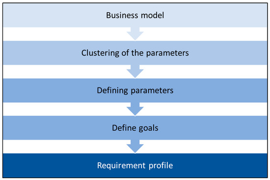
Figure 3.
Procedure for drawing up the requirements profile for pay-per-x applications.
The pay-per-x business model in mechanical engineering depends largely on the integration of measurement technology and sensors. These instruments are crucial for collecting precise data on the use, performance and condition of machines. Their use enables transparent and fair billing based on actual performance parameters. The integration of measurement and sensor technology therefore plays a key role in the success and effective implementation of this innovative business model.
Gap analysis therefore plays a crucial role in evaluating existing sensor technology in terms of its suitability for integration into pay-per-x business models. A comparison is made between the existing sensor technology and the previously defined parameter space (“billing-relevant parameters”, “process transparency”, “extended service”) in order to subsequently check whether the existing sensor technology can map the defined parameters using measurement technology.
In the event that gaps are identified during the gap analysis with regard to the sensors required to create suitable process transparency, a market analysis is carried out to identify suitable sensor technology to close these gaps. The task is then to define the requirements for suitable sensor technology and then to research this sensor technology with a final technical and economic evaluation. Here too, reference should be made to the sensor selection concept described in Section 3 of this text, which provides a useful selection aid when researching suitable sensors.
As soon as suitable sensor technology is available, it makes sense to draw up a measurement and integration concept for the sensor technology suitable for the pay-per-x business model, in which the following requirements are defined:
- Measurement conditions: Based on the requirements and specifications of the sensor technology, the installation location and type are defined and the environmental conditions permissible for the sensor technology are checked.
- Measuring section concept: A concept for the entire measuring section (signal acquisition, conversion and forwarding) is drawn up. All transmission elements and interfaces must be defined.
- Data acquisition: The transfer of the measurement signals to the data acquisition system must be defined.
- The measured variables must be recorded, with which the billing-relevant parameters and process transparency can be quantified.
2.5. Evaluation Methods
Evaluation methods in the pay-per-x business model are necessary to analyze various aspects of usage:
- Billing accuracy: The pay-per-x business model is based on customers paying for actual usage or results achieved. Evaluation methods enable the precise measurement and evaluation of these parameters, which ensures accurate billing.
- Performance monitoring: Evaluation methods allow providers to monitor the performance of their products or services. This makes it possible to identify potential problems at an early stage, optimize efficiency and increase customer satisfaction.
- Adaptation of the offer: Evaluation methods enable providers to adapt their offers based on the actual needs and requirements of customers. This helps to provide a competitive and customer-oriented service.
- Contract design: When defining contract terms in the pay-per-x business model, it is important to make agreements based on well-founded evaluations. This creates transparency and trust between providers and customers.
The evaluation methods relate to the data recorded by the measurement technology/sensor technology. The development of evaluation algorithms for recorded sensor data is necessary in order to
- (a)
- limit the amount of data to a necessary level through data aggregation, and
- (b)
- quantify the service provided according to the billing-relevant parameters in line with the respective business model.
The task includes the conceptual development of procedures and tools for data aggregation and analysis. Aspects such as the assessment of data quality, the handling of outliers and/or data gaps, the selection of possible methods for data aggregation, the normalization of data and the selection of possible methods for data analysis are taken into account. The result should be a concept for data aggregation and an evaluation of the recorded parameters—a concept for data evaluation.
The following questions have proven to be helpful when analyzing the recorded process data:
- Are the sensors and the measuring section reliable?
- Are all values available?
- Are there any outliers?
- Are the recorded values plausible?
- Is the sampling frequency sufficient?
- What impact do the consumption data have on the business model?
2.6. Process Windows and Interdependencies
It is essential to develop a methodology for deriving process windows as part of the pay-per-x business model. This involves assigning clear limits to the defined parameters, which must be adhered to by the operator in order to avoid overloads and reduce higher loads and wear and tear. The development of a procedure to take these higher loads into account, in particular their interdependencies, is crucial. It should also be noted that the definition of and compliance with these process windows have not only technical but also financial implications. The cost structure is directly influenced, as overloading can lead to increased wear and possibly higher maintenance or repair costs. It should be noted that if the process windows are exceeded, the user will be faced with higher costs, as this can lead to additional burdens and potential financial implications. Therefore, a comprehensive development strategy that takes into account both technical and financial considerations is required to ensure a sustainable implementation of the pay-per-x business model that balances efficiency and longevity with financial profitability.
2.7. Testing, Evaluating and Adapting the Selected Sensors
As part of the development of a pay-per-x business model, the sensor technology to be used is of crucial importance and must function flawlessly. The aim is to test, evaluate and adapt the selected sensors and evaluation methods. This can be realized at a laboratory level or, even better, at the respective application. The task includes the development and realization of test setups for each sensor in order to test and evaluate their intended use. The process reliability and measurement accuracy of the sensor application are of crucial importance.
The generated data are then processed using the developed concepts for data evaluation, and the resulting findings are evaluated in terms of their informative quality. The final result consists of the evaluation of the tested sensors, the evaluation methods and the methods for defining process windows and cause–effect relationships.
3. General Concept for Selecting Sensors
In this section, a procedure is presented that enables users to select suitable sensors depending on their particular application.
As every user formulates their own criteria when selecting sensors, the aim of this guide is to present a standard strategy that covers as broad a field of applications as possible and can therefore be used individually. Accordingly, the procedure shown below is also kept general.
Several established approaches to sensor selection in industrial applications form the basis of the method proposed in this paper. Hesse and Schnell [6] present a systematic selection process that focuses on the functional requirements of sensors (e.g., resolution, linearity and response time), technical environmental conditions and economic and operational factors. These include, among others, the evaluation of interference factors, protection classes, temperature resistance, service life and installation conditions. The work in [6] also provides a structured sequence for sensor evaluation—from selecting the physical sensing principle and defining the measurement range to analyzing installation requirements and fieldbus connectivity. Furthermore, sensor principles are classified according to their access type (point, surface, etc.) and typical sensing distances depending on the operating principle.
The VDMA Industry 4.0 guideline [7] also recommends a systematic approach to sensor selection, which is based on identifying sensor functions and developing a requirement profile for each sensor. In addition, Panick and Marré (2022) [8] propose a retrofit concept for sensors in networked production systems, focusing particularly on data availability and the potential for process integration.
The methodology developed in this paper extends these established approaches by introducing a coherent decision framework specifically tailored to the requirements for process transparency and the implementation of usage-based business models (e.g., pay-per-X). In addition to technical suitability, economic parameters such as resource costs, retrofit capability and the monetization potential of measurable variables are systematically integrated into the selection process. This enables a direct link between technical measurement variables and managerial control objectives.
3.1. The Selection Cycle
Before a sensor system is procured and used in practice, it is necessary to make preliminary considerations. The following selection cycle (Figure 4) is suitable for this purpose.
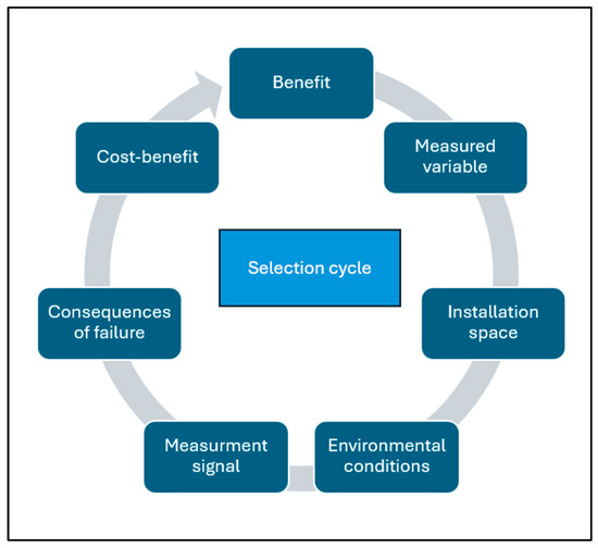
Figure 4.
Choosing sensors by using the selection cycle.
In the selection cycle presented here, the first step is to formulate the value proposition (benefit) behind the selection of a particular sensor and the associated type of data acquisition and information generation. This involves answering the fundamental question of what information is required to realize the benefit and, based on this, in the second step, which measured variable must be recorded for this purpose.
In the third step, the restrictions imposed by the installation space of the component must be determined and taken into account when selecting the sensor. The questions to be answered are where the optimum mounting location for the sensor is located or where the disturbance variables for the measurement are minimized (or in other words, where the generation of the measurement signal achieves optimum quality), and whether or how the sensor can be mounted there.
The location of the data processing will also have to be taken into account. This can take place in the sensor element itself, in the sensor housing or in various stages outside the housing.
Similar to the location of the data processing, the provision of the data, and subsequently the information, is characterized by the proximity or distance to the measurement location, whereby it must be determined who receives access rights to the data.
It must be determined for which persons/functions it makes sense to access the data—this ranges from the machine operator (proximity to measuring location) to the external service provider (distance to measuring location).
The fourth step, which is closely linked to the installation space, involves determining the environmental conditions and ensuring good signal quality over the long term. This includes protecting the sensor from external influences and ensuring that it can be used permanently even under difficult conditions (e.g., at very high temperatures, in liquid and gaseous media, etc.). Table 6 shows a comparison of different sensor types and failure examples.
Table 6.
Comparison of different sensor types and possible issues.
In the fifth step, the properties of the measurement signal for the planned data interpretation should be determined, such as the quality of the measurement signal—i.e., the recording of values that are as free as possible from disturbance variables.
In order to record signals that are as interference-free as possible, minimum requirements of the measurement signal are formulated for the respective measured variable, such as the decision as to whether absolute or relative values are measured, as well as whether measured values are recorded continuously or at intervals. In addition, the type of signal to be used must be decided for its respective application: an analog, digital or binary signal?
Furthermore, decisions must be made regarding the sampling frequency, the resolution of the measured values and whether real-time capability is required or even feasible.
In the sixth step, users must deal with possible failures and their consequences, which can be caused by failed sensor functions or sensors in a fault state. This includes determining the possible consequences of failure, assessing and evaluating risks and hazards, and planning countermeasures.
In the seventh step, the originally formulated benefit or objective is used to analyze the relationship between the benefit and the anticipated costs (cost–benefit analysis).
In general, the sensor selection cycle is designed in such a way that the successive steps provide users with a systematic approach that can also be run through individually as required.
If the cost–benefit analysis reveals that the costs are too high or the benefits are only minor, the cycle can be run through iteratively, i.e., it is repeated until the user approaches a satisfactory solution.
All or individual modules can be revised when the cycle is repeated. If, for example, only one building block or individual building blocks need to be revised for a satisfactory cost–benefit ratio or an optimization loop, these have no influence on the previous steps.
3.2. The Building Blocks of the Selection Cycle
3.2.1. Measured Variable, Measuring Principle and Measuring Method
This module of the selection cycle concerns the selection of the measured variables or the physical variables to which the measurements apply. A distinction must be made here between the directly measured variable (e.g., the Hall voltage with a Hall effect sensor) and the indirectly derived variable that is of actual interest to the user (e.g., the rotational speed of a shaft or the position determination using a Hall effect sensor).
In order to achieve the desired goal, suitable measured variables and corresponding measuring principles and measuring methods must be selected. In this way, suitable sensors can be narrowed down without having to consider mechanical integration (installation space) or the measurement signal at this point. The latter two steps are carried out later—a premature determination in this respect would only limit the user’s selection options.
Based on the benefits and the existing technical systems, there are various principles for determining the measured variables.
Depending on the measurement principles and methods considered, the focus will be on different effects and conditions. These can be recorded in various ways by determining them directly, indirectly, via another measured variable or by correlating a number of other variables.
Starting with the selection of suitable measurement variables, measurement principles and measurement methods, it is advisable to answer the following questions:
- Which variables should be measured?
- Which measurement principles should be used and which measurement methods are available?
- Are the measured variables static or dynamic?
- In which area is a sensor to be used?
- Are the physical operating principles of the sensor suitable for determining the measured variable? What are the advantages and disadvantages of these principles?
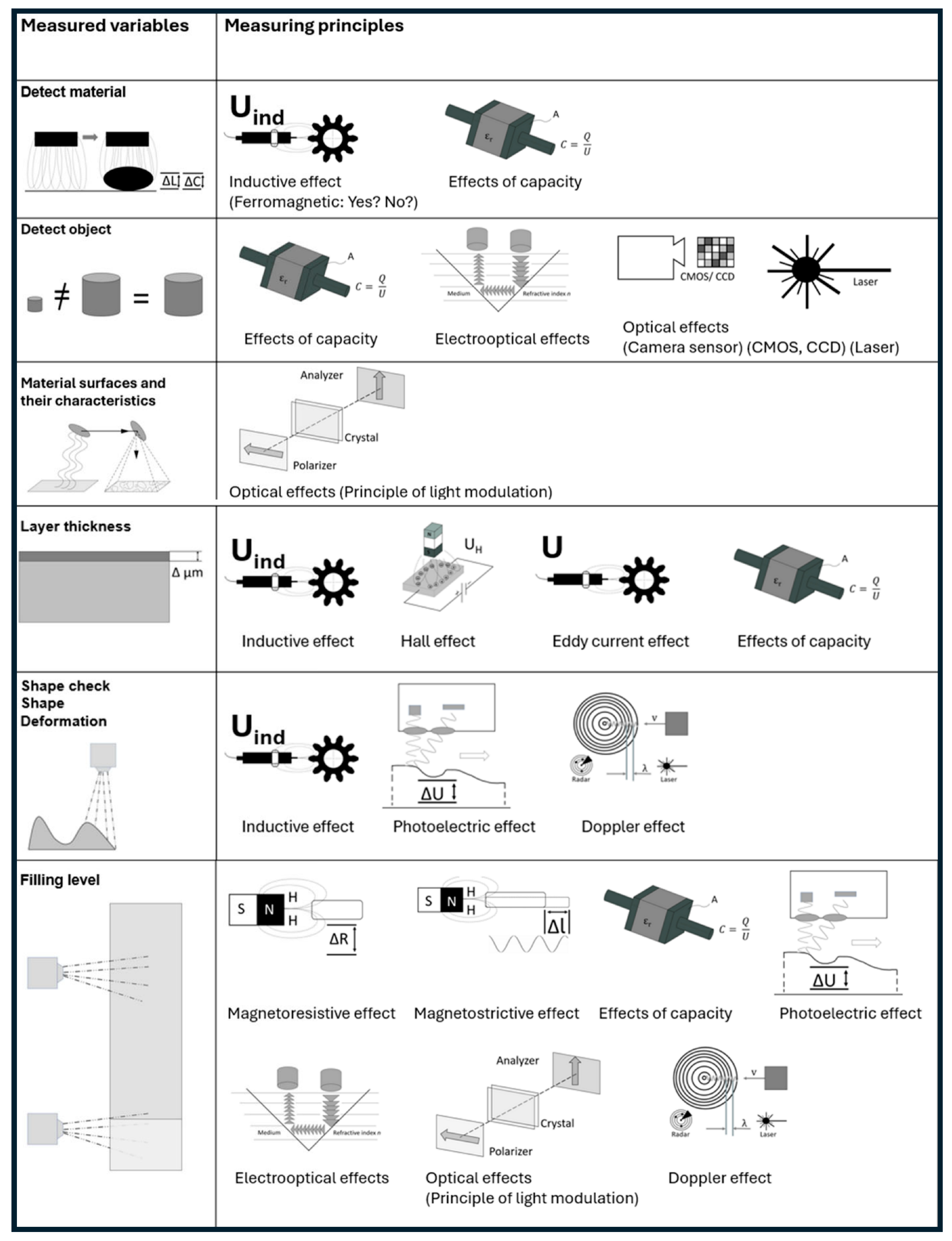
Overview of the Measuring Principles and the Variables That Can Be Measured with Them
When making a selection, it is advisable to use the overview of measured variables and the corresponding measuring principles presented here. The most important physical effects and measuring principles that can be used for measuring purposes in this overview are only presented here as an overview that does not claim to be exhaustive and is focused on the areas of mechanical engineering and manufacturing. Before going into more detail on the selection of existing measurement principles for the measurement of a specific measurand, here is an overview of measurement principles and the measurands that can be determined using these principles. See also Hering and Schönfelder [16]. Occasionally, overlaps between the different categories cannot be avoided. See the twenty physical effects in Table A1.
When selecting measurement variables and principles, it is advisable to consider as many options as possible—even the less preferred ones—since the measurement method may be restricted later when the installation space is considered due to the associated environmental conditions, which may require protective measures for the sensors, for example in [17].
The physical effects known to us and that are useable for measurements (measuring principles) are directly limited to the following physical quantities:
- Resistance R;
- Electrical voltage V;
- Current I;
- Capacitance C;
- Inductance L;
- Charge Q;
- Frequency f;
- Time t.
Indirectly, a number of other measured variables—i.e., information—can be obtained, such as the following:
- The interrelated variables: Force, pressure, torque;
- Absolute temperature, temperature difference;
- Position, distance, path, angle, rotational speed and angular and linear velocity. (The acceleration can be determined by changing the position, distance, path and angle);
- Acceleration;
- Flow rate;
- Quantities of audible sound and structure-borne sound;
- Distinguishment between different materials;
- Recognition and differentiation of objects;
- Recognition and differentiation of surfaces and their properties;
- Layer thickness and material thickness;
- Recognition and differentiation of shapes and deformations;
- Level detection;
- And other variables.
These sizes can in turn be differentiated according to the following criteria, whereby overlaps are possible:
- Geometric quantities;
- Mechanical measured variables;
- Time-based measurands;
- Absolute temperature and temperature differences (contact thermometry, radiation thermometry);
- Electrical and magnetic measurands;
- Acoustic measurands;
- Optical, photoelectric and electro-optical measurands;
- And other variables.
In the following, further considerations regarding sensor selection will be demonstrated using a use case. In this use case, the speed or rotational speed of a driving three-phase motor of any machine tool is to be determined. The following possible options are available for a selection of measuring principles:
- Induction effects;
- Eddy current effect;
- Hall effect;
- Magnetoresistive effect.
Based on the use case selected here, the measurement principles mentioned are briefly presented and discussed.
Effects of Induction: Inductive Sensor/Inductive RPM Sensor
An inductive sensor is an electromagnetic sensor and uses a magnetic field to measure changes in the distance between the sensor and the measurement object—only measurement objects made of ferromagnetic materials come into consideration here. The sensor contains a coil that is wound around a magnet and causes a change in the magnetic flux and the coil when, for example, the teeth and the base of a gearwheel alternately pass the sensor. The moving cogwheel generates a varying magnetic flux, which induces a proportional voltage—the inductive voltage—in the coil (Figure 5). The frequency of this inductive voltage is related to the speed and generates a sinusoidal signal whose amplitude depends on the target variable (magnetic flux or induced voltage), the speed and the distance (between the sensor tip and the target).
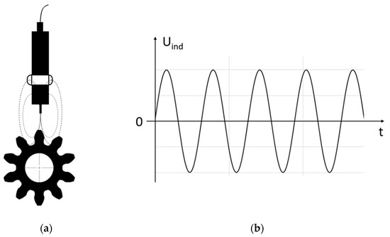
Figure 5.
(a) Schematic measurement setup for an inductive sensor and gear wheel; (b) sinusoidal output signal.
The use of inductive sensors for speed measurement can be disadvantageous if the speed is too low, the gear tooth is too small or the distance to the measurement object is too large, which means that the signal is too flat and can therefore no longer be used [18]. An example of a sinusoidal signal flattened in this way is shown in Figure 6.
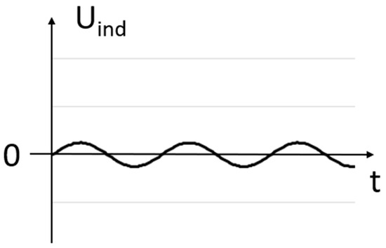
Figure 6.
Flattened sinusoidal signal.
However, this measuring principle can only be used if the measurement object—in this case a drive shaft of a three-phase motor—has corresponding ferromagnetic incremental sensors/markings (the teeth on a gear wheel), as the inductive voltage only arises due to a change in the magnetic field. If there were no markings on the shaft and therefore no changes in the distance between the sensor and the object during a rotation, no change in the magnetic flux and therefore no inductive voltage could be measured.
It would then be necessary to fit a corresponding pulse wheel or incremental wheel with reference mark(s) on the shaft.
Eddy Current Effect: Eddy Current Sensors
In an eddy current sensor, an alternating current feeds the coil, generating an alternating magnetic field. As soon as this field penetrates an electrically conductive material, a current with closed, circular current lines is generated—this is the so-called eddy current. This eddy current in turn generates a magnetic field in the material, which counteracts and inhibits the original magnetic field of the coil. As soon as the distance between the sensor tip and the material changes, the original magnetic field of the coil also changes. A change in distance causes a change in the impedance of the coil. This change is measured by means of the voltage U applied to the coil (Figure 7), whereby the distance value (usually in mm) is displayed as the output. A sinusoidal output signal is also generated here.

Figure 7.
(a) Schematic measurement setup—eddy current sensor and gear wheel; (b) sinusoidal output signal.
In principle, measuring the speed of a gearwheel using the eddy current effect would work in the same way as with the aforementioned inductive sensor, so that a tooth is measured or counted at a short distance and a tooth gap at a greater distance. Here too, the shaft would have to have a pulse wheel or incremental wheel with reference mark(s).
However, one advantage of eddy current sensors over inductive sensors is that not only can ferromagnetic measurement objects be measured, but also all materials that are electrically conductive.
The use of eddy current sensors for speed measurement can be disadvantageous if the gear tooth moves at too high a speed and the eddy current sensor hardly recognizes any differences in distance, in which case the sine line becomes increasingly flattened (see Figure 6). This means that when using eddy current sensors, attention must be paid to how high the speed could be and whether a meaningful signal can still be generated.
Hall Effect: Hall Effect Sensors
A Hall effect sensor (named after Edwin Hall) detects changes in the magnetic flux between the integrated magnet and the material of the target and reproduces these changes in the form of the so-called Hall voltage UH (electrical voltage), which represents the measurement signal. The material of the target must be electrically conductive. Semiconductors are preferably used for this purpose [6].
Hall effect sensors are sensitive to external magnetic fields. As shown in Figure 8, Hall effect sensors directly output electronically evaluable square wave signals. This is an advantage over inductive sensors because the signals must first be processed.

Figure 8.
(a) Schematic measurement setup—Hall effect sensor and gear wheel; (b) rectangular output signal (square wave signal).
Since the signal voltage of Hall effect sensors is independent of speed, they have a wide measuring range and can therefore correctly detect not only fast-moving targets, but also slow and static conditions. Again, a pulse wheel or incremental wheel with a reference mark must be attached to the shaft.
Magnetoresistive Effect/Magnetoresistive Sensor
A magnetoresistive effect occurs when an external magnetic field is applied to a material through which a current is flowing and the electrical resistance in the material changes as a result. The material must be electrically conductive. The intensity of the resistance change is described by the difference between resistance RH (resistance with magnetic field H) and resistance R0 (resistance without magnetic field H). R0 serves as the reference value:
The magnetic force component of the Lorentz force FL causes the electrons to be deflected from their original path, and their path through the measurement object is extended, thus increasing the resistance R.
Here too, a pulse wheel or increment wheel with a reference mark must be attached to the shaft.
Notes on the Pulse Wheel and Direction of Rotation Detection
The teeth of a gear wheel can be used as a pulse/increment wheel without the need for additional design work. For a shaft that does not have such increments, a so-called pole ring or encoder ring can also be integrated, on which magnets are arranged. These magnets take over the function of the teeth of an incremental gear, thus fulfilling a prerequisite for speed measurement.
In addition, the direction of rotation can also be detected without much effort. The magnets are arranged alternately at the north and south poles on a pole ring or encoder ring. With such an arrangement of magnets (or increments), it is possible to detect the direction of rotation. This requires an internal signal offset, which is realized by at least two correspondingly arranged sensors.
The detection of the direction of rotation is made possible by the internal signal offset of three correspondingly arranged Hall elements in the sensor. In such a wheel speed sensor, magnets take over the function of the teeth of the incremental wheel. The magnets are divided into north and south poles and are arranged alternately on a pole ring (encoder ring).
The measurement method:
All four measurement principles—induction, eddy current, Hall and magnetoresistive effect—first generate analog signals (analog measurement), which are converted into digital signals by means of evaluation electronics (digital measurement).
In the case of Hall sensors, the signal-processing electronics are integrated in the immediate vicinity of the elementary sensor (transducer) in the same housing and not outside the housing at a greater or lesser distance from the elementary sensor.
3.2.2. Installation Space
Deciding too early in favor of a specific or a few specific measurement methods before the installation space has even been examined can prove to be a premature step if, for example, the installation space is nevertheless too small or inaccessible for the intended sensors. However, it can also mean that unnecessary considerations are made regarding design changes to the sensor housing or the selection of an alternative sensor type.
The restrictions may include the nature of the structural installation space, the existing or missing interfaces for communication and the power supply, or interfaces that have yet to be created.
Mounting options for the sensor solution must also be considered. In connection with this, it is necessary to examine where and how fastenings are possible or not possible, or which disadvantages bring a certain advantage.
It is also important to consider the size and weight of the sensor and whether it needs to be interchangeable and calibrated.
The latter point (interchangeability and calibration) may mean that a sensor can be physically integrated into the technical system, but its accessibility is limited—making maintenance difficult or even impossible without resulting in significant downtime.
How and where the sensor is attached to the technical system must also be considered, as the question of where the measurement is taken determines the possible influence of sources of interference and can reduce the quality of the measurement signal and the significance of the data generated later. The choice of measurement location can mean that a sensor is subject to different external influences, and even the sensor housing, which is intended to protect the sensor system from precisely these, can itself become a disturbance variable and distort the measurement result, e.g., due to the natural frequency or excessive mechanical damping [7].
The installation space of the technical system also has an influence on the mechanical integration of the sensors themselves: If there are opportune possibilities to integrate a sensor into existing housings or circuit boards of the technical system, these should be localized and evaluated. As long as the quality of the measurement signal is not reduced and the processes in the technical system are not hindered, existing integration options for the sensor should be preferred.
The question of how the data are to be processed and further transported and which requirements for the communication technology are sufficient, e.g., whether the data are to be communicated wirelessly or with a corresponding cabling effort, should also be discussed at this point. Considerations about the topology (line, ring, star, tree, point-to-point), the range of the connection or the length of the cable, the transmission speed and the cycle time (possible requirement for real-time capability) should be made when considering the installation space because the environmental conditions and the properties of the measurement signal are considered in the next steps.
The location of the data processing is also crucial. This can take place in the sensor element itself, in the sensor housing or in various degrees outside the housing—whether in an additional external evaluation component/module, in the machine controller, in the company’s local or central server/computer center, or completely externally on servers/computer centers of a service provider (cloud).
Similar to the location of the data processing, the provision of the data, and subsequently the information, is characterized by the proximity or distance to the measuring location: the information/data can be provided directly at the sensor, outside the machine, in the machine controller or operator terminal, in the company’s local or central server/computing center, in the MES/ERP system or in the cloud.
Not everyone needs to have full access rights to the data. This point is also characterized by proximity vs. distance, with the difference that graduated options are possible here: the machine operator receives the information necessary for his activities, while the other users of the company’s own IT network, the machine manufacturer or another external service provider (e.g., external maintenance staff, material suppliers, customers, etc.) receive more or less complete access rights—and this is all depending on the benefit formulated at the beginning.
3.2.3. Environmental Conditions
When selecting a sensor, it is essential to determine the environmental conditions so that the sensor element is protected from external influences. This point is again related to the installation space and the quality of the measuring signal depending on the measuring location. Even if the measuring location guarantees sufficient signal quality, it is far from certain how long a sensor can withstand these conditions. For example, a measurement under water (or another medium) may require a sensor housing to remain sealed for as long as possible. In this case, not only is the choice of sensor type crucial but also that of its housing in order to ensure perfect functioning.
In this interaction of sensor type and sensor position, the external conditions must be taken into account and determined—these can be temperature, relative humidity, pressure, vibration or shock, acceleration, electrical/magnetic interference fields and others [18].
3.2.4. Measuring Signal
The properties of the measurement signal determine the quality with which the data are processed and subsequently interpreted. Quality here means that, as far as possible, only that which was intended to be measured is measured, and if disturbance variables are measured, these must be identified and filtered out [19]. At the very least, it should be possible to recognize interfering factors and distinguish them as irrelevant variables from the relevant measurement data when interpreting the data.
In order to record signals that are as interference-free as possible, minimum requirements for the measurement signal must be set for the respective measured variable.
The measured variables can be recorded in absolute terms or via the relative change in the measured variable. It may also not be necessary for a measurement signal to be constantly processed or transmitted. In other cases, however, this may be possible depending on the application.
The type of signal determines how the signals are processed and later interpreted. The application determines whether analog signals (e.g., via the display of a pressure gauge or float of a flow measurement), digital signals (discrete signals with a specific sampling frequency and resolution) or binary signals (zero or one, on–off, such as a light grid as a protective measure) are to be used.
The goal is to generate interpretable signals.
To achieve this, the performance of the data processing must be thought through, such as the required sampling frequency and resolution, the necessary computing operations and the cycle time (possibly also the requirement for real-time capability, i.e., that an event is responded to within a precisely defined maximum period of time).
3.2.5. Consequences of Failure
The question of the consequences of a failure or fault condition of the sensor system should be addressed by the company determining the potential failure consequences of the system or product. They should then estimate and evaluate the risk and develop suitable countermeasures for a fail-safe. A Failure Mode and Effects Analysis (FMEA) can be used for this purpose.
Fail-safe development can have different priorities. For example, safety-critical applications to protect people’s health and lives come first, and only then do process control applications come into focus in terms of process capability, component quality and cycle time.
A failure of the sensor system is not the worst case scenario but can occur if the sensor system appears to be working correctly but is no longer able to correctly reflect the status of the process or product, and this is in an error state, so that faulty components are produced unnoticed. The later the error is discovered in the process chain, the greater the costs.
Maintenance measures must be considered here to ensure that the sensors continue to function properly. The costs for this are probably far below the possible failure and consequential failure costs.
Though the maintenance and inspection effort cannot be determined from the outset, they must be investigated. The reliability of the sensor system must be examined. Reliability is the ability to fulfill a required function under given conditions for a given period of time and is a statistical variable. A probability variable can therefore to be interpreted with a certain degree of uncertainty [20].
Linked to this is the service life of sensor elements or sensor systems. The service life can be equated with the probability of failure or the probability of survival, and investigations must also be carried out here.
Additional functionalities that do not disrupt the value-adding process, or only present a time delay, should also be subject to a risk assessment with the necessary initiation of maintenance measures, but are unlikely to result in failure, and their consequential failure costs are as high as those mentioned above.
3.2.6. Cost–Benefit Analysis
As mentioned above, a formulated benefit can be set against the expected costs, and a decision can be made as to whether a technically feasible solution for the sensor system is also economically viable. The selection cycle does not have to end here if it is uneconomical, but can be continued iteratively, e.g., at the building block in the selection cycle, at the decision node where an improvement in economic efficiency is assumed.
In addition to the economic factors, other factors will also play a role in the cost–benefit analysis, e.g., the maintenance effort (servicing, inspection and repair), operational safety, the reliability and service life of the sensor components and electronics, the cabling or wireless network, the other peripherals, the cost of qualified employees who can interpret the information and an external service provider who takes over these tasks.
The selection cycle can be created in its entirety as a project if it represents a complex and novel task.
3.3. Application Example
The above-mentioned cycle for selecting suitable sensors is explained below using a practical example. The first step is to define the benefits of the sensor technology. It describes what information is required to achieve the objective. In this example, a calculation increment is to be determined for a pay-per-x business model of a modular peeling unit for wire drawing machines (Figure 9). In this case, this is the drawn and peeled wire length.

Figure 9.
Principle sketch of a wire drawing machine with modular peeling unit (red).
In the next step, a measured variable is defined that is required to be able to draw conclusions about the wire length. One way of determining the wire length is to record the drawing speed of the wire as it passes through the tool. This is specified as an input parameter on the drawing machine.
This results in two scenarios for the installation space, which is defined in step 3. On the one hand, the parameter can be tapped directly via the machine’s PLC, but this requires a great deal of effort. To avoid in-depth intervention in the existing machine, the actual speed of the wire can be measured tactilely, for example, using a measuring wheel encoder. With a measuring wheel encoder, the movement is recorded via a friction wheel that rests on the surface of the measured object and converts it into speed values. In the fourth stage of the selection cycle, the respective environmental conditions that can have an influence on the sensor technology are considered. In the case of the measuring wheel encoder, this includes contamination, for example, from the drawing lubricant. This can lead to slippage, i.e., “slipping”, due to a lack of friction between the target and the measuring wheel, resulting in inaccurate measurement. Other influences are the vibrations of the measuring object and wear of the measuring wheel due to contact with the measuring object, which occurs in the form of adhesion and abrasion. In the worst case, this can lead to damage to the drawn material, making this measuring system unsuitable for use in this example.
As the exclusion of the aforementioned sensor type in the first run was due to the external influences caused by the tactile measurement, the third step is to be revised for the second iteration loop. The aim is therefore still to determine the wire length by recording the drawing speed. However, this measured value recording should now take place without contact on the measurement object. Laser velocimeters, for example, are used for non-contact speed measurement. These have the advantage that they record movement without having to change the surface of the measurement object, for example, by applying a scale. According to DIN EN 60825-1 (VDE 0837-1): 2015-07 [21], which specifies safety requirements for laser products and aligns with the international standard IEC 60825-1:2014, lasers are divided into different laser classes (1, 1M, 1C, 2, 2M, 3R, 3B and 4) depending on their hazard potential. This classification system helps to define the necessary safety measures, labeling, and protective requirements to mitigate risks from hazardous laser radiation. For example, Class 3B defines a laser whose radiation is dangerous to the eye and skin, while Class 1 describes a non-hazardous laser that poses no risk under normal operating conditions [22].
However, the function of the laser velocimeter can also be limited by some environmental influences. For example, they are dependent on the surfaces of the object being measured. For example, temperature fluctuations or heterogeneous adhesions of the drawing material can impair its reflection properties and thus falsify the measurement results. In addition, the measured distance can vary due to vibrations of the drawing material during the process, which can lead to measurement uncertainties. This type of sensor is therefore also unsuitable for measuring the drawing speed to determine the drawn wire length.
As it was not possible to develop a successful sensor concept in the previous iterations by measuring the speed, the second step, the definition of the measured variable to be recorded, is to be revised for the third iteration loop. Another way to determine the wire length is to directly measure the speed of the capstan or drawing disk. A measuring wheel encoder, whose friction wheel rests on the capstan, can also be used for this purpose. As in the first iteration, however, slippage due to drawing agent residue and wear due to abrasion of the measuring wheel on the capstan wall can also occur here, which means that high measuring accuracy cannot be guaranteed.
Figure A1 and Figure A2 provide assistance in selecting suitable measuring principles for the respective measured variables. For example, capacitive, inductive or eddy current sensors can be used for speed measurement. Table 7 shows the advantages and disadvantages of the measuring principles. Based on this comparison, an inductive sensor is selected below to measure the speed of the capstan without contact. These have a long service life and remain unaffected by operating material residues from industrial practice, such as lubricants or lubricant carriers.
Table 7.
Advantages and disadvantages of different sensor types.
In step 5, the properties of the measurement signal are defined, which form the basis for data processing. The following questions need to be answered:
- Are absolute or relative measured values required?
- Which type of signal is required? (Binary, analog or digital.)
- How high should the sampling frequency be?
- What measurement accuracy is required?
- Should real-time data be recorded?
For example, relative measured values are sufficient for determining the wire length s by determining the speed n, as only the speed difference in the time window t must be considered in order to be able to draw conclusions about the drawing speed. In this case, d is the diameter of the capstan from which the average speed is recorded.
Furthermore, digital, i.e., discrete, measured values are sufficient. This is mainly due to the sampling frequency. The practical example presented here is a drawing machine with a maximum drawing speed of 300 m/min. This results in a capstan speed of less than 150 rpm, at which even lower sampling frequencies of up to 1 kHz provide a good result. The measuring accuracy of inductive sensors is indicated by the hysteresis loss, which depends on the switching distance of the sensor. In this example, the measurement accuracy is set at ±3% and no real-time data need to be available, as the wire length is only calculated for the subsequent determination of costs according to the pay-per-x model.
The penultimate stage of the selection cycle deals with the question of the consequences of a sensor failure and how to react to it. To be on the safe side, an inductive sensor was selected in advance, as these are generally very robust and have a long service life. These sensors are also insensitive to dirt, which keeps maintenance costs low. The last point is additionally supported by IO-Link as the current standard in sensor technology, as it is not necessary to intervene in the control system programming to replace a sensor. If the sensor is identical in construction, it can even be replaced very easily via “plug-and-play” [23].
The selection cycle concludes with a consideration of the cost–benefit ratio. The acquisition costs of inductive sensors are in the lower price segment. In addition, the installation and maintenance costs mentioned above are low with a long service life and good measurement results. This means that integration for data acquisition is achieved with little effort and cost, resulting in a good cost–benefit ratio and the completion of the selection cycle. An overview of the respective iteration loops and the associated questions of the selection cycle is shown in Figure 10.
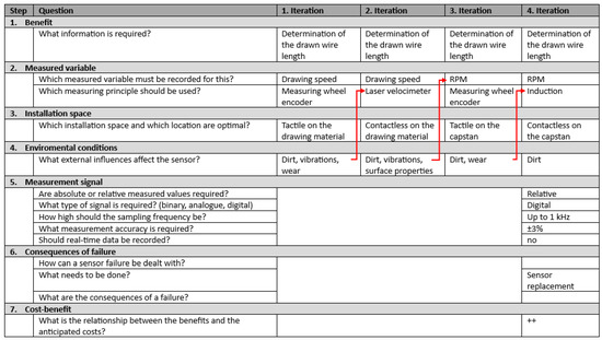
Figure 10.
All iteration loops of the selection cycles (Arrows show the iterative optimization process during sensor selection by visualizing the changes between iterations, ++ represents a quantitative evaluation of the relationship).
4. Conclusions
The transparent recording and analysis of process parameters is a key success factor for modern production environments and data-driven business models such as pay-per-use. This guide provides a structured approach to selecting and implementing appropriate sensor technology to ensure reliable process visibility. By systematically analyzing relevant measurements, considering environmental conditions and evaluating signal processing, companies can make informed decisions about sensor selection.
Particularly in the context of pay-per-use models, the accurate and traceable recording of usage and utilization parameters is crucial to ensure fair billing and long-term profitability. The methods presented for sensor selection and process monitoring help to identify existing measurement gaps and implement suitable solutions.
In the long term, the targeted use of sensor technology not only enables greater operational efficiency but also provides the basis for further applications such as predictive maintenance or data-driven optimization in production. Companies that use these guidelines can analyze, evaluate and develop their processes in a targeted manner—a decisive step towards smarter and more flexible production.
Author Contributions
Conceptualization, S.I. and M.M.; methodology, P.K., S.I. and M.M.; validation, P.K., S.I. and M.M.; writing—original draft preparation, P.K., S.I. and M.M.; writing—review and editing, S.I., M.M. and P.K.; visualization, S.I. and P.K.; supervision, M.M.; project administration, M.M.; funding acquisition, M.M. All authors have read and agreed to the published version of the manuscript.
Funding
This review was created as part of the joint research and development project “Condition assessment and process assistance for service life-based business models to increase flexibility in production (ZuPro2Flex)”, funded by the German Federal Ministry of Education and Research (BMBF) within the program “The Future of Value Creation – Research on Production, Services and Work” (funding numbers 02K18D090 to 02K18D099) and managed by the Project Management Agency Karlsruhe (PTKA). Additionally, this article was funded by the Open Access Publication Fund of the South Westphalia University of Applied Sciences.
Data Availability Statement
No new data were created or analyzed in this study. Data sharing is not applicable to this article.
Acknowledgments
The authors would like to thank the German Federal Ministry of Education and Research (BMBF) for funding this research and development project within the framework of the program “The Future of Value Creation—Research on Production, Services and Work”, managed by the Project Management Agency Karlsruhe (PTKA). Special thanks go to Daniel Panick for his preparatory work on the project and for documenting the results during his time as research assistants at our laboratory.
Conflicts of Interest
The authors declare no conflicts of interest.
Appendix A
Table A1.
Overview of the twenty physical measuring effects.
Table A1.
Overview of the twenty physical measuring effects.
|
|
|
|
|
|
|
|
|
|
|
|
|
|
|
|
|
|
|
|
Appendix B
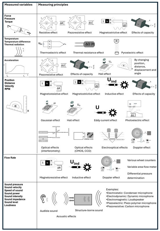
Figure A1.
Selection of the measuring principle based on the measured variable (part 1).
Figure A1.
Selection of the measuring principle based on the measured variable (part 1).
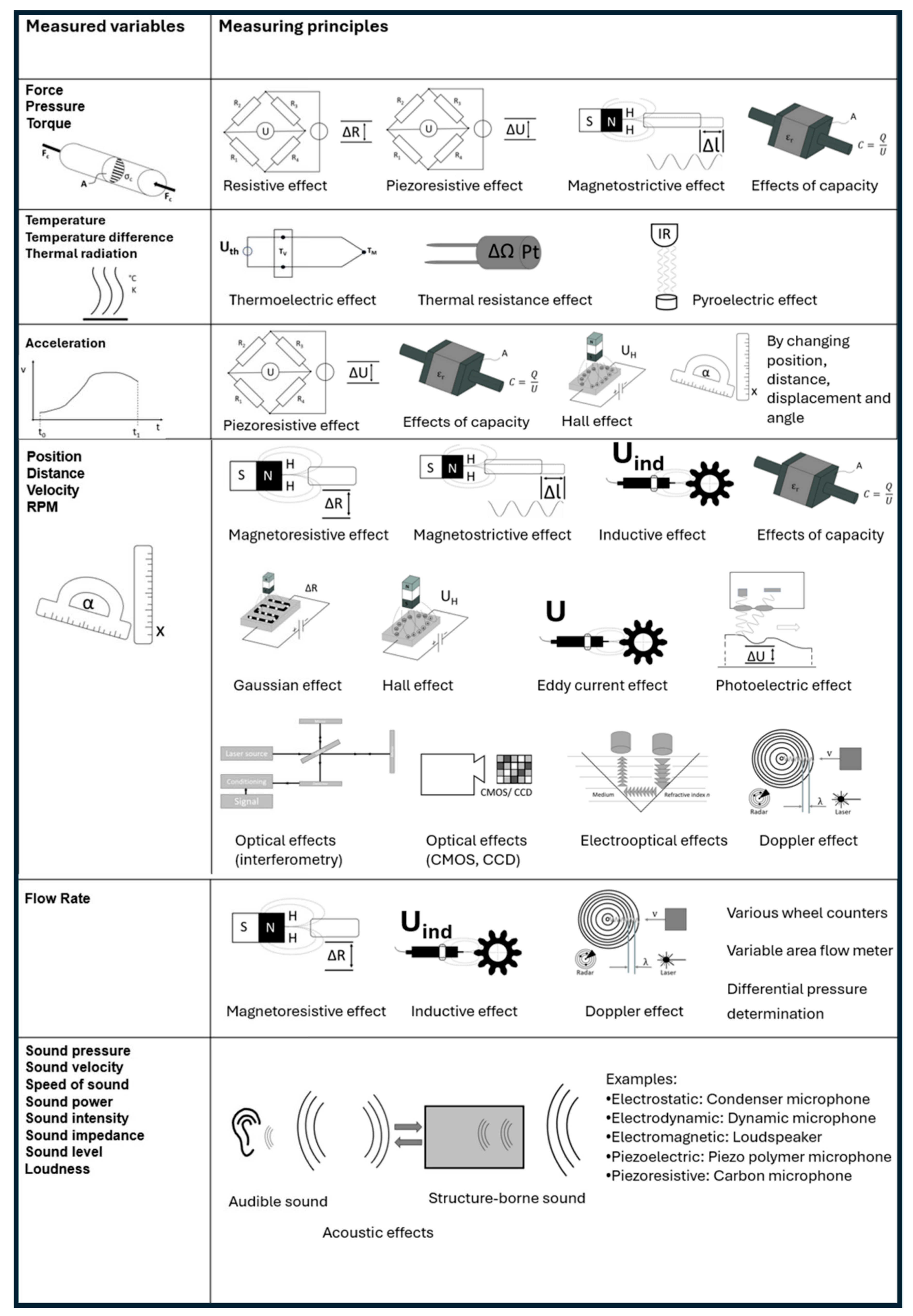

Figure A2.
Selection of the measuring principle based on the measured variable (part 2).
Figure A2.
Selection of the measuring principle based on the measured variable (part 2).
References
- Singer, A. ZuPro2Flex: Zustandsbewertung und Prozessassistenz für Nutzungsdauerbasierte Geschäftsmodelle zur Flexibilitätssteigerung in der Produktion. Available online: https://produktion2x.de/ (accessed on 16 January 2025).
- Alaluss, M.; Drechsler, C.; Kurth, R.; Mauersberger, A.; Ihlenfeldt, S.; Marré, M.; Labs, R. Usage-based leasing of complex manufacturing systems: A method to transform current ownership-based into pay-per-use business models. Procedia CIRP 2022, 107, 1238–1244. [Google Scholar] [CrossRef]
- Osterwalder, A.; Pigneur, Y.; Clark, T.; Smith, A. Business Model Generation: A Handbook for Visionaries, Game Changers, and Challengers; Wiley: Hoboken, NJ, USA, 2010; ISBN 9780470876411. [Google Scholar]
- Bundesministeriums für Wirtschaft und Klimaschutz. Existenzgruendungsportal des Bundesministeriums für Wirtschaft und Klimaschutz. Available online: https://www.existenzgruendungsportal.de/ (accessed on 23 November 2024).
- BusinessPilot GmbH. Business Model Canvas: Nutzen, Beispiel, Anleitung. Available online: https://gruenderplattform.de/geschaeftsmodell/business-model-canvas-beispiele (accessed on 4 December 2024).
- Hesse, S.; Schnell, G. Sensoren für Die Prozess—und Fabrikautomation: Funktion—Ausführung—Anwendung, 7th ed.; Springer: Wiesbaden, Germany, 2018; ISBN 9783658211738. [Google Scholar]
- Fleischer, J.; Spohrer, A.; Klee, B.; Merz, S. Leitfaden Sensorik für Industrie 4.0: Wege zu kostengünstigen Sensorsystemen; Verband deutscher Maschinen-und Anlagenbau, Karlsruher Institut für Technologie, Eds.; VDMA Forum Industrie 4.0: Frankfurt, Germany, 2018. [Google Scholar]
- Panick, D.; Marré, M. Konzept zur Sensornachrüstung: Messdaten als Basis zur Kollaboration im Produktionsnetzwerk. Z. Wirtsch. Fabr. 2022, 117, 896–901. [Google Scholar] [CrossRef]
- Franco, C.; Acero, J.; Alonso, R.; Sagues, C.; Paesa, D. Inductive Sensor for Temperature Measurement in Induction Heating Applications. IEEE Sens. J. 2012, 12, 996–1003. [Google Scholar] [CrossRef]
- García, C.A.R.; Große, N.; Haehnel, H. Taschenbuch der Automatisierung, 3rd ed.; Fachbuchverlag Leipzig im Carl Hanser Verlag: München, Germany, 2017; ISBN 3446446648. [Google Scholar]
- Pohl, R.; Casperson, R.; Thomas, H.-M. Mögliche Fehlerquellen und deren Einflüsse bei der Risstiefenbestimmung mit Wirbelstrom; Own Publisher BAM: Berlin, Germany, 2009. [Google Scholar]
- Schmidt, W.-D. Sensorschaltungstechnik, 3rd ed.; Vogel Buchverlag: Würzburg, Germany, 2007; ISBN 9783834360656. [Google Scholar]
- Pitsch, H. Informationserfassung durch Galvanomagnetische und Strukturierte Komponenten in Sensorsystemen. Ph.D. Thesis, Universität Duisburg-Essen, Duisburg, Essen, Germany, 2003. [Google Scholar]
- Fraden, J. Handbook of Modern Sensors: Physics, Designs, and Applications, 5th ed.; Springer International Publishing: Cham, Switzerland, 2016; ISBN 9783319193038. [Google Scholar]
- Dorf, R.C.; Bishop, R.H. Modern Control Systems, 13th ed.; Pearson Education Limited: Harlow, UK, 2017; ISBN 9781292152974. [Google Scholar]
- Hering, E.; Schönfelder, G. Sensoren in Wissenschaft und Technik: Funktionsweise und Einsatzgebiete, 2nd ed.; Springer: Wiesbaden, Germany, 2018; ISBN 9783658125622. [Google Scholar]
- Dumitrescu, R.; Koldewey, C. (Eds.) Datengestützte Produktplanung: Mit Betriebsdaten und Data Analytics zur Faktenbasierten Planung Zukünftiger Produktgenerationen im Produzierenden Gewerbe; Heinz Nixdorf Institut Universität Paderborn: Paderborn, Germany, 2023; ISBN 9783947647279. [Google Scholar]
- Hüning, F. Sensoren und Sensorschnittstellen; De Gruyter: Berlin, Germany, 2016; ISBN 3110438550. [Google Scholar]
- Bechtloff, J. Messtechnik, 1st ed.; Vogel Buchverlag: Würzburg, Germany, 2011; ISBN 9783834361493. [Google Scholar]
- Tränkler, H.-R.; Reindl, L. Sensortechnik Handbuch für Praxis und Wissenschaft Hans-Rolf Tränkler, 2nd ed.; Springer: Berlin/Heidelberg Germany, 2014; ISBN 9783642299414. [Google Scholar]
- Deutsches Institut für Normung e.V. Safety of Laser Products: Part 1: Equipment Classification and Requirements (IEC 60825-1:2014). 2022 (60825-1). Available online: https://www.dinmedia.de/de/norm/din-en-60825-1/344085844 (accessed on 4 March 2025).
- Schneeweiss, C.; Eichler, J.; Brose, M.; Weiskopf, D. Leitfaden für Fachkundige im Laserschutz: Hilfe bei der Durchführung der Gefährdungsbeurteilung nach OStrV, 1st ed.; 2020; Springer Spektrum: Berlin/Heidelberg, Germany, 2020; ISBN 9783662612422. [Google Scholar]
- Uffelmann, J.R.; Wienzek, P.; Jahn, M. IO-Link: Brückentechnologie für Industrie 4.0; Vulkan-Verlag GmbH: Essen, Germany, 2018; ISBN 9783835673786. [Google Scholar]

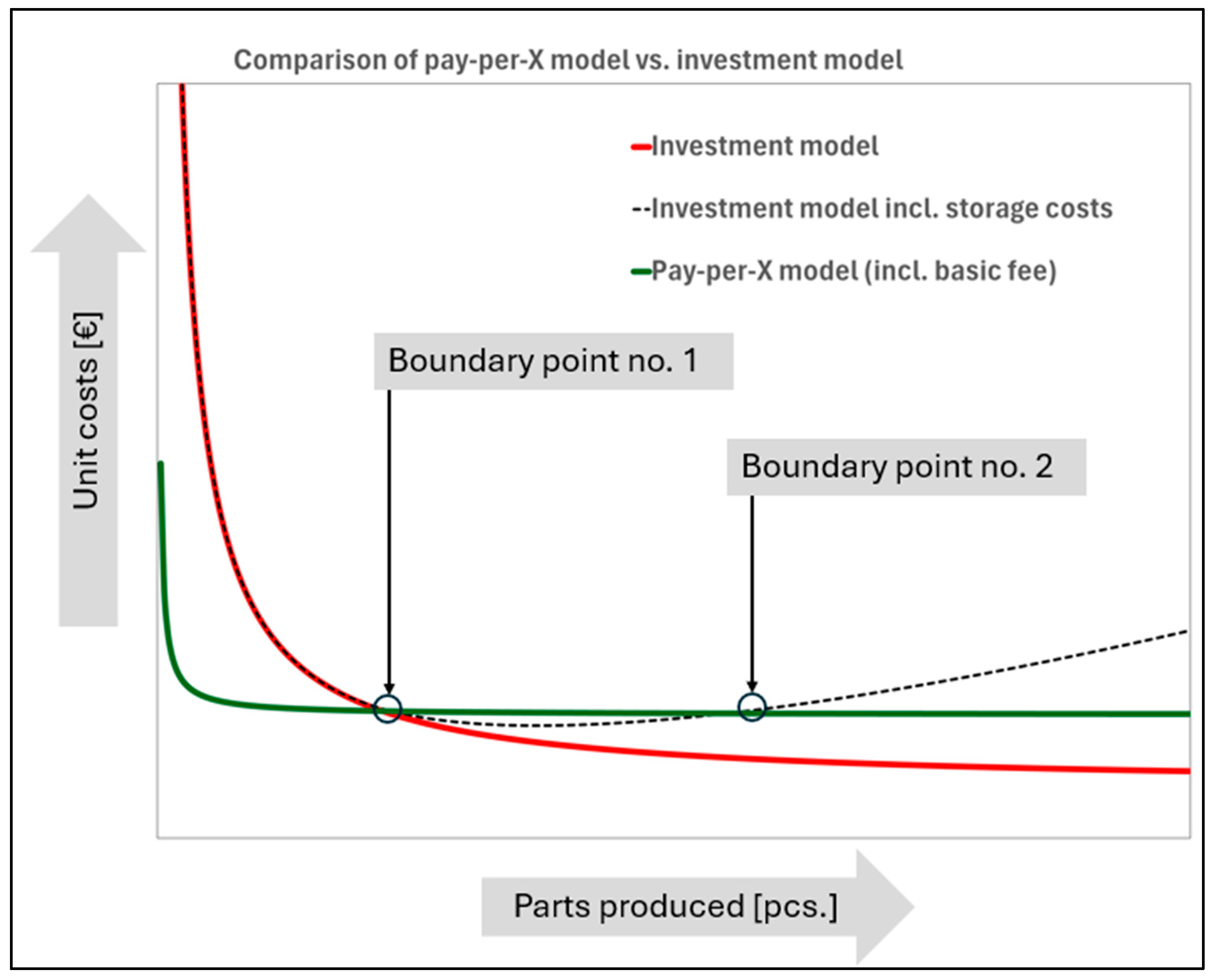
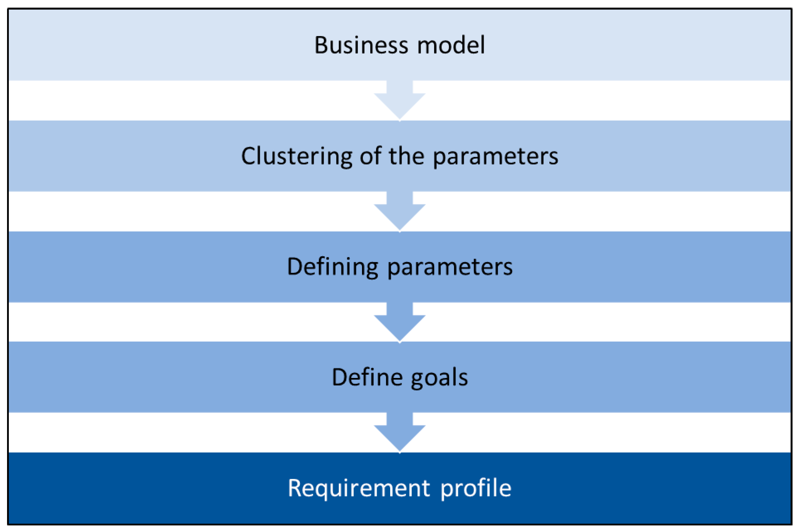
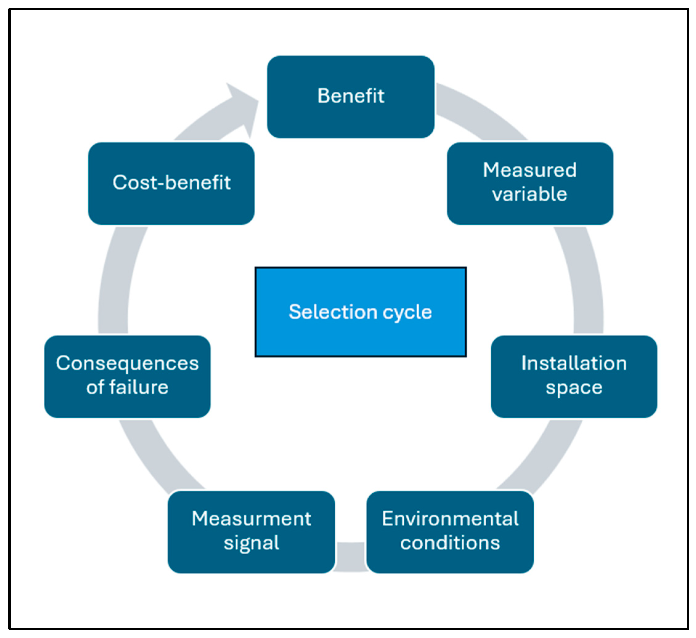


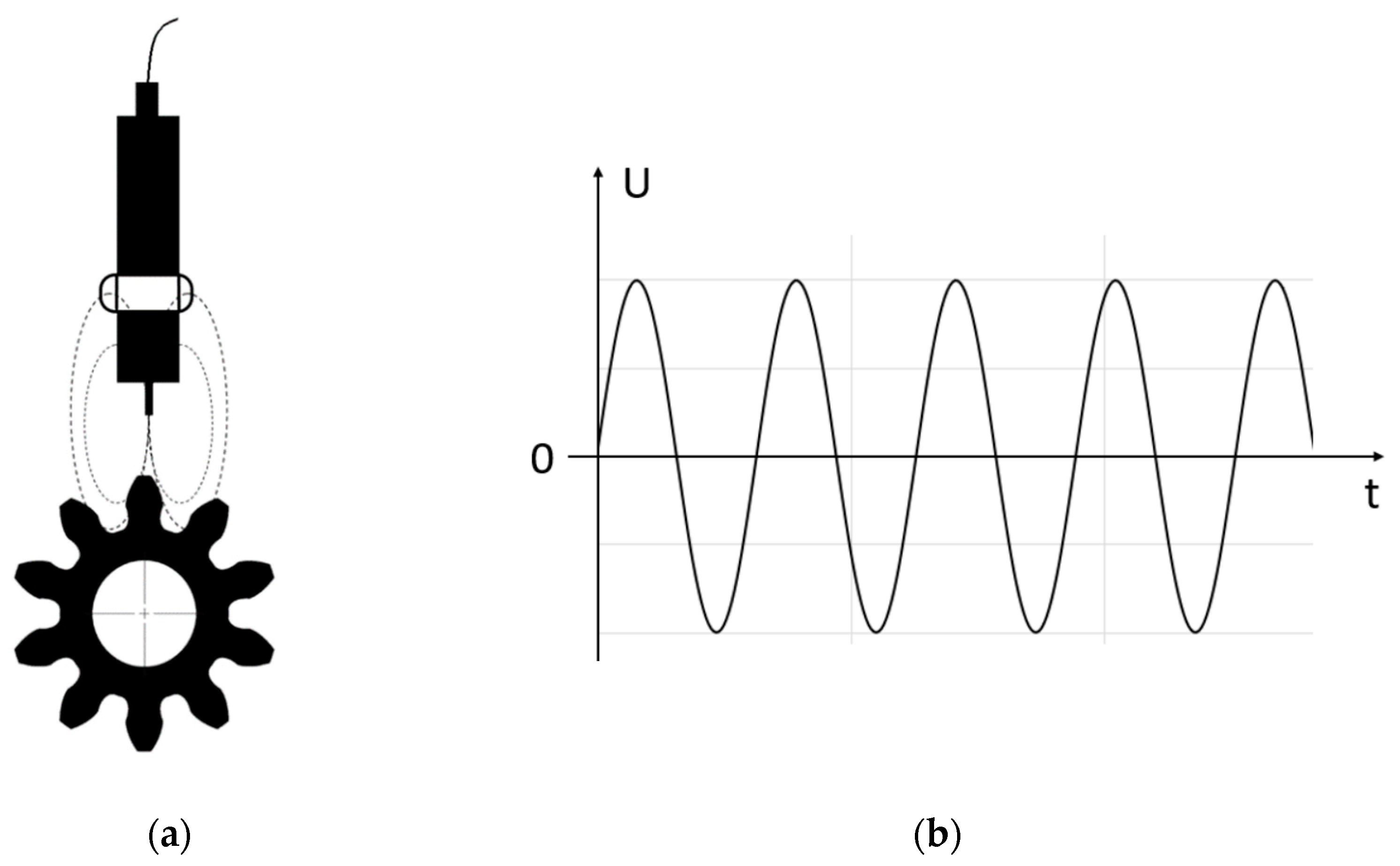
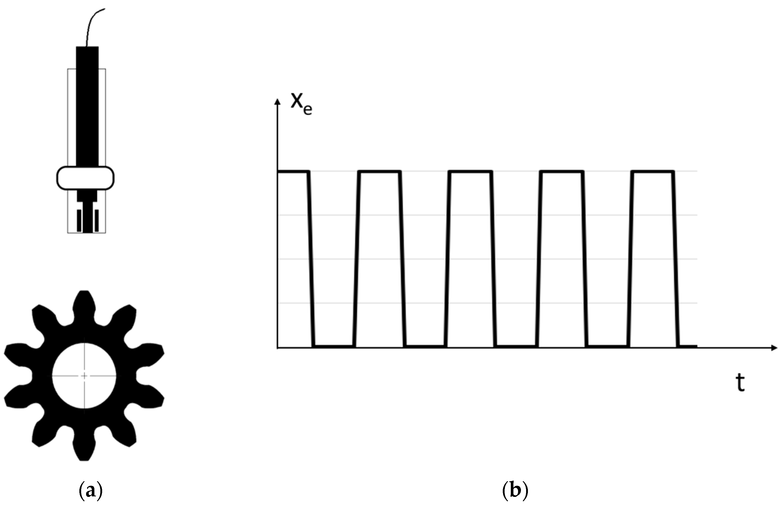
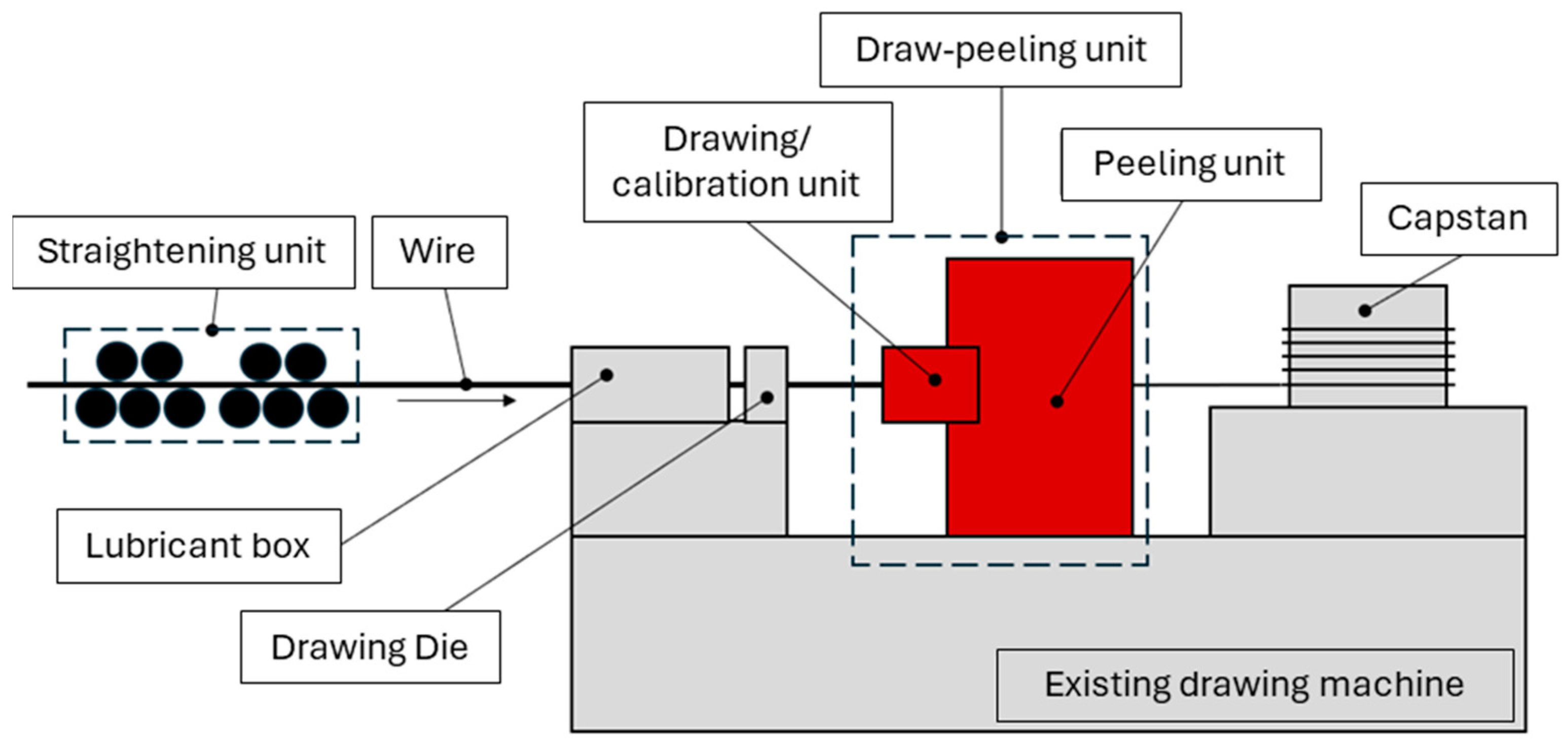
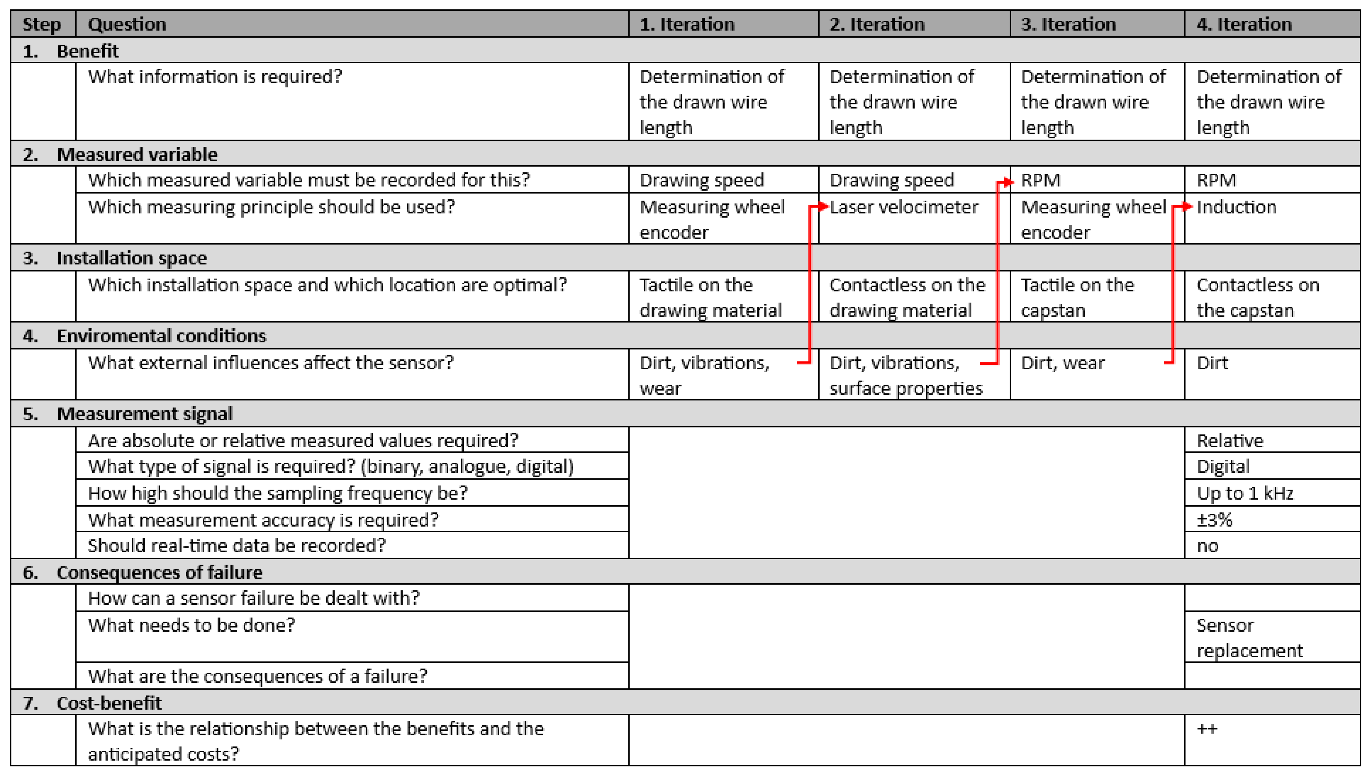
Disclaimer/Publisher’s Note: The statements, opinions and data contained in all publications are solely those of the individual author(s) and contributor(s) and not of MDPI and/or the editor(s). MDPI and/or the editor(s) disclaim responsibility for any injury to people or property resulting from any ideas, methods, instructions or products referred to in the content. |
© 2025 by the authors. Licensee MDPI, Basel, Switzerland. This article is an open access article distributed under the terms and conditions of the Creative Commons Attribution (CC BY) license (https://creativecommons.org/licenses/by/4.0/).