4.1. Branch Line Fault Location
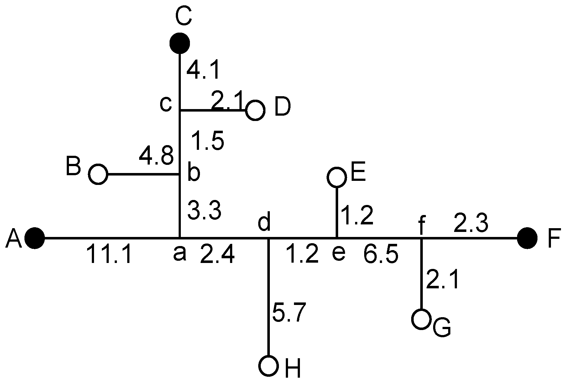
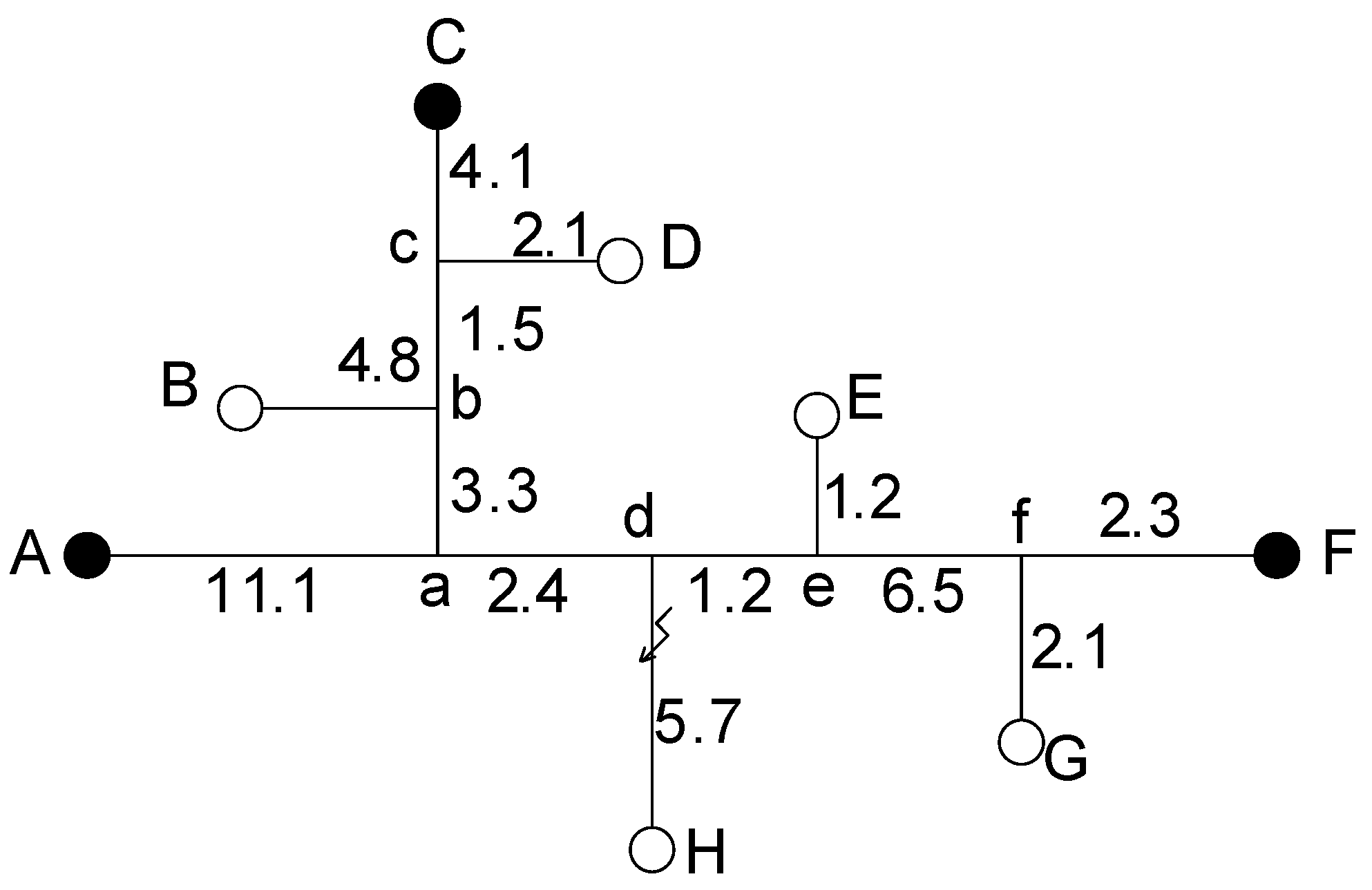
Assume the fault occurs at the “dH” branch line section, 4.1 km away from H point. The traveling wave detection device is installed at the distribution transformer at the end of the distribution line to extract the voltage traveling wave. The distribution network fault topology is shown in
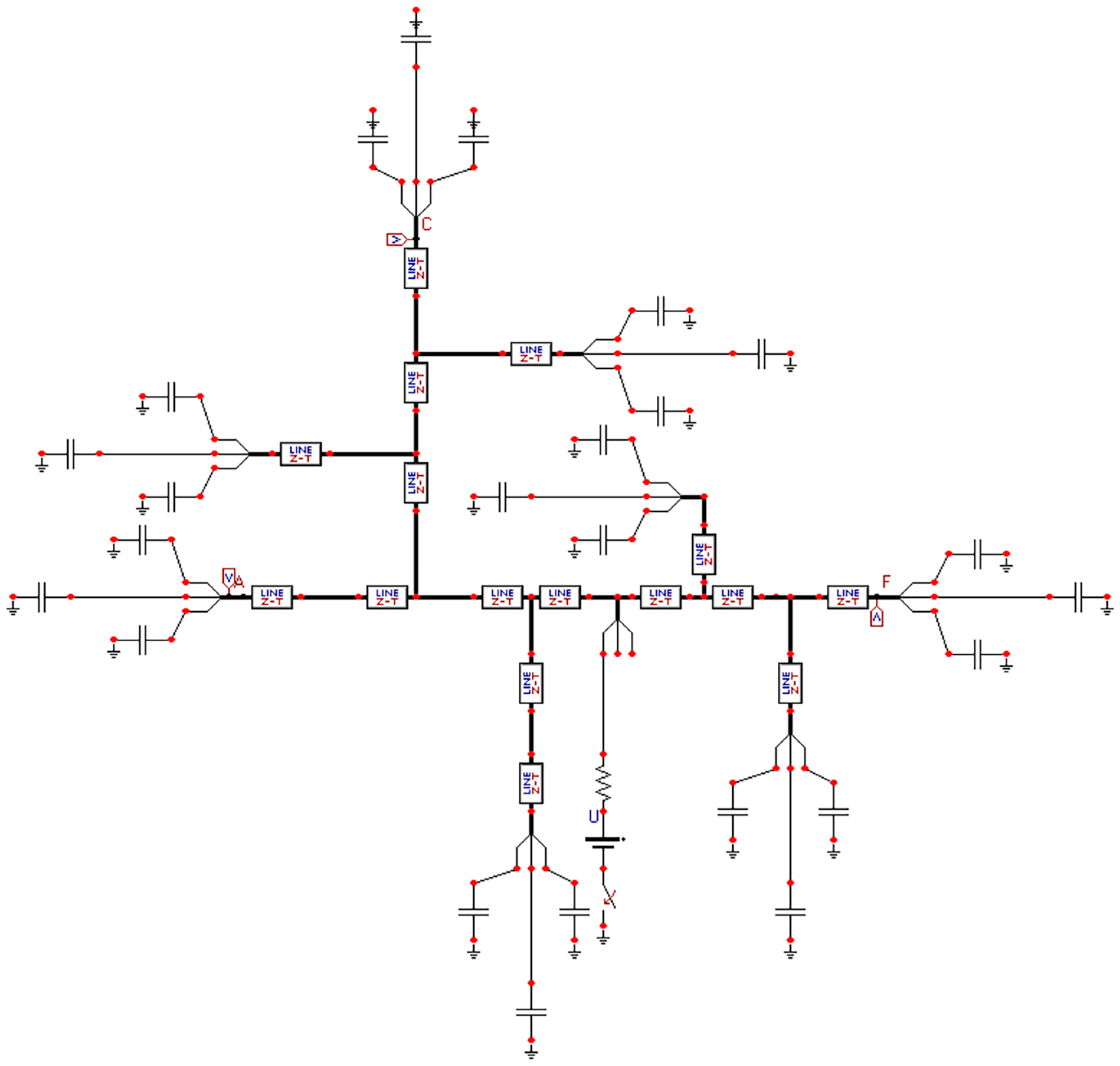
Figure 5. The fault model of the simulated distribution network was drawn in ATP simulation software, as shown in
Figure 6.
A,
C, and
F are the detection points of the three detection devices. The fault is set as a single-phase ground fault, the occurrence time is set to 0 s, the simulation step size is set to 1 × 10
−8 s, and the total simulation time is set to 800 μs. The simulation waveforms of the traveling wave reaching detection points
A,
C, and
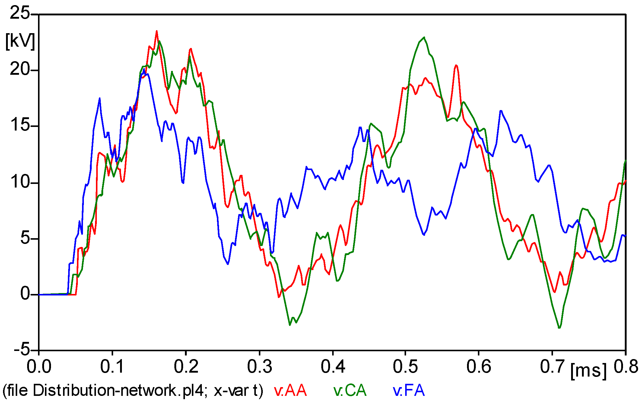
F are shown in
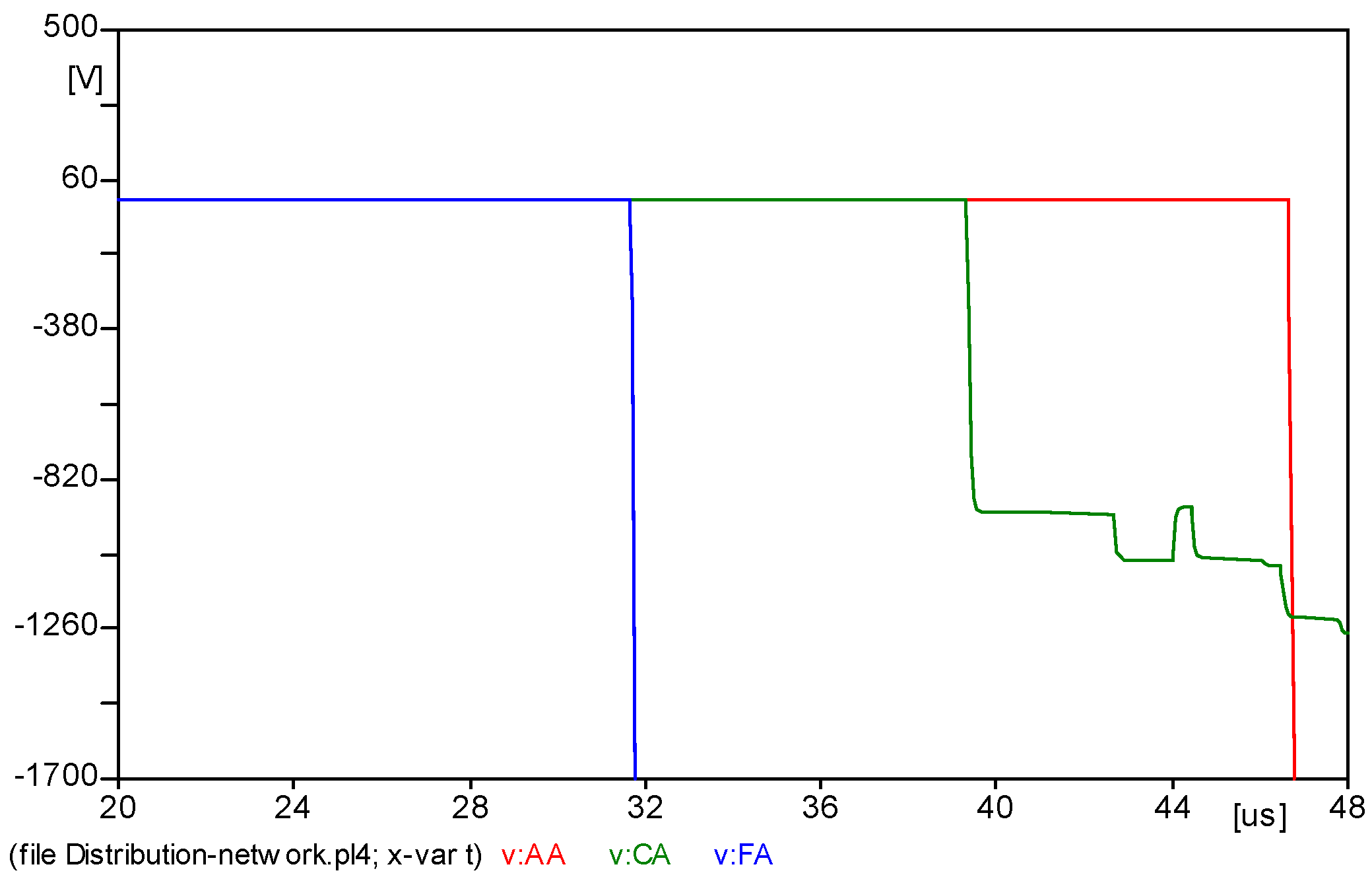
Figure 7. It can be seen from the figure that the initial wave head time of the waveform is very close, so it is impossible to accurately identify the initial time of the wave head. It is necessary to amplify the initial traveling wave head signal, as shown in
Figure 8.
As can be seen from
Figure 8, when the traveling wave head signal is calibrated, the initial time for fault traveling wave head transmission to detection point
A is 50.3 μs, the transmission time to detection point
C is 42.95 μs, and the transmission time to
F detection point is 38.65 μs. Then, we input the time when the fault traveling wave arrives at
A,
C, and
F into the program, compare it with the time database traversal of fault traveling wave arrival at the detection device, and filter to match the range of sections. The program simulation fault point is located in the U
7 section, which proves that the fault occurred on this branch.
Detection devices
A and
F at both ends of the main line are used to extract the initial signal of the wave head and perform double-terminal positioning to calculate the fault distance. The length of
lAF is 23.5 km. The distance from fault point
f to node
A is:
Because the fault point is located in the U
7 section (dH section), as determined by the program, the time from the intersection point d of the dH section branch to detection device
A is 45 μs, and the distance from the fault point
f to the intersection point
d of the branch is:
The distance between the fault point of the branch line and detection device A is the double-terminal positioning value plus the distance from the fault point to the intersection point of the branch line: 13.498 + 1.59 = 15.088 km. The actual distance between the fault point and detection device A is 11.1 + 2.4 + 1.6 = 15.1 km. The positioning calculation error is 12 m.
4.3. Branch Intersection Node Fault Location
Assuming the fault occurs at point
f of section fG of the branch intersection node 21.2 km away from point
A, the simulation model diagram of the distribution network fault is shown in
Figure 11.
The initial wave head is amplified to
A,
C, and
F, as shown in
Figure 12. The transmission time of the fault traveling wave to detection point
A is 70.69 μs, the transmission time to detection point
C is 63.34 μs, and the transmission time to detection point
F is 7.67 μs. The time when the fault traveling wave arrives at
A,
C, and
F is entered into the program and compared with the time database of the fault traveling wave arrival detection device. After screening, we determined that the fault point is located in the U
12 section of the branch line.
When considering a branch intersection node f fault, theoretically, node f belongs to the three connected sections fG, fF, and ef (U10, U11, U12 sections). Because of the existence of time errors in traveling wave detection, the section positioning cannot fully locate the fault point; it can only locate it in a certain section near the node. Database comparison and positioning are only for the U12 line section. Therefore, a certain margin needs to be set for the positioning of the branch intersection node to ensure the fault tolerance of the fault location. The fault distance is calculated through the double-terminal positioning method of the detection device.
The distance from fault point
f to detection device
A is:
The fault point of the traveling wave positioning is the main line U12, and the actual fault point f is 21.2 km away from A. The branch intersection node cannot be accurately identified. There is a positioning deviation at the node, but the traveling wave positioning error is only 3 m. Onsite maintenance personnel can still find the accurate branch intersection node near the fault point, and within the allowable positioning error range, fault positioning can also be achieved.
Based on the simulation experiments, this fault location method has a maximum error of 12 m and a minimum error of 3 m in locating the branch line, main line, and branch intersection node, and it can achieve accurate fault location. Three traveling wave detection devices are used in this article. When a certain traveling wave detection device on the main line loses data and fails to locate due to a fault, it can be switched to another traveling wave detection device, which improves the fault tolerance and reliability of fault location.
Using the branch line fault simulation model as described before, we conducted a simulation analysis of different fault types. Three different short-circuit types, namely, a two-phase short-circuit, a two-phase short-circuit grounding, and a three-phase short-circuit, which occurred 4.1 km away from the H point, were taken as an example. The positioning results are shown in
Table 5.
The occurrence of a single-phase fault was taken as an example for simulation under different transition resistances. The transition resistances were set from metal grounding to high-resistance grounding from small to large, and different transition resistances, such as 1 Ω, 100 Ω, and 1000 Ω, were used 4.1 km from the H point. The positioning results are shown in
Table 6.
The fault initial phase angles were adjusted to 15°, 30°, and 60°. The positioning results are shown in
Table 7.
Next, we adjusted the positions of different fault points separately. We selected the ad section of the main line 12 km away from detection device
A, the de section of the main line 14 km away, and the Bb section of the branch line 16 km away. The positioning results are shown in
Table 8.
According to the above simulation positioning results, the position errors of the rural distribution networks are all within 30 m, which can meet the requirements of fault positioning accuracy.
In addition, after the same number of positioning devices was configured, the time information matching the multi-terminal traveling wave fault positioning method proposed in this paper was compared with the new fault positioning method combined with two traveling wave principles and the D-type positioning method [
22]. Fault points were set for the main lines and branch lines, and simulation verification was carried out under different transition resistances and fault initial phase angles. The positioning results are shown in
Table 9.
As can be seen from the comparison of the location results in
Table 9, when a fault occurs in the main line, if the fault point is in the “ad” section of the main line, it is 12 km away from the
A detection device. The maximum positioning error of this algorithm is 30 m, and the maximum error of the new fault location method combined with two traveling wave principles and the D-type location method is 46 m. The three methods mentioned above can achieve accurate fault location. However, with the time information matching multi-terminal traveling wave fault location method proposed in this paper, by using multiple sets of time constraints, the fault point can be uniquely determined by comparing and traversing the time array. Then, fault location can be achieved by using double-terminal traveling wave positioning, which has high accuracy and a small error. Overall, the maximum positioning error is reduced by 34.8%.
Table 9 also shows a fault that occurs in the branch line, where the fault point is in the branch line section “Bb”, which is 16 km away from the
A detection device. Because of the need to extract zero-mode and linear-mode wave velocities through phase-mode transformation, inaccurate extraction of zero-mode and linear-mode waves can lead to positioning errors. Therefore, the fault location method based on the combination of two traveling wave principles has a large positioning error, and the accuracy is within the range of 0.341 km. The D-type positioning method has a false fault point, and when the fault point is a branch point of the branch line, the absolute error is 1.555 km. In addition, the error value is too large, which made the method fail. In contrast, the positioning error of the method proposed in this paper is within 35 m in all cases, which accurately determines the fault location.
This method is less affected by the fault location, transition resistance, and initial phase angle of the fault, and it has high positioning accuracy. Therefore, the time information matching multi-terminal traveling wave fault location method proposed in this article has the characteristics of a simple process and accurate positioning, which can meet the requirements of precise fault location in rural distribution networks.
However, in actual distribution networks, different types of lines have different wave speeds. The aging of the line and an increase in temperature can lead to an increase in wire resistance, a decrease in wave speed, and intensified signal attenuation and distortion, making it more difficult to accurately detect time and affecting positioning accuracy. It is necessary to combine multi-dimensional methods, such as signal processing and equipment status evaluation, to effectively improve positioning accuracy. The initial wave head signal of a traveling wave has noise interference in detection, which can easily confuse the wave head characteristics and submerge the signal. The interference of the wave head signal can directly lead to measurement errors in the arrival time of the wave head, affecting the accuracy of traveling wave positioning. Filtering and preprocessing are needed to remove noise and interference and improve robustness in noisy environments. The distribution network needs to manually readjust each section to the detection device time database due to changes in line length, but it cannot be automatically updated in real time. There are positioning deviations at the intersection of branches, which affect accuracy and require consideration of fault tolerance. Therefore, further research is needed.


