Optimized Bi-LSTM Networks for Modeling Ni(II) Biosorption Kinetics on Quercus crassipes Acorn Shells

Abstract

Heavy metal pollution from anthropogenic sources poses significant risks to ecosystems and human health. Biosorption offers a sustainable removal method, but kinetics are poorly captured by traditional neural networks. This study introduces optimized Bidirectional Long Short-Term Memory (Bi-LSTM) networks for multivariate modeling of Ni(II) biosorption on Quercus crassipes acorn shells, trained using experimental (EKD), synthetic (SKD), and combined (CKD) datasets. A two-stage hyperparameter optimization with Optuna yielded models with R² above 0.995 and low RMSE in 5-fold cross-validation. Second-stage models showed high stability, with coefficient of variation (CoV) values below 10% for RMSE. Based on unseen kinetics, production models showed slightly lower performance (R² = 0.89–0.996): EKD1, EKD2, and CKD1 showed the most consistent performance across challenging conditions with R² values of 0.9617, 0.9769, and 0.9415, respectively; SKD models achieved strong results under standard conditions (kinetic 1, SKD1 R² = 0.9963). SHapley Additive exPlanations (SHAP) analysis identified contact time and initial Ni(II) concentration as key variables, with temperature, cation charge, and a salt interference code also contributing to model interpretability. These findings demonstrate that optimized Bi-LSTM networks offer a robust and interpretable data-driven solution for modeling Ni(II) removal under multivariate conditions, including the presence of salts.

1. Introduction

Water pollution is a critical environmental issue that poses severe threats to human health, biodiversity, and aquatic ecosystem balance [1,2]. The rapid pace of industrialization and urban expansion, as well as intensified agricultural activities, have introduced diverse pollutants into water bodies, including excess nutrients, pathogens, persistent organic pollutants, and heavy metals [3,4].

Industrial effluents are pivotal to water contamination because their complex composition often exceeds the self-purification capacity of natural water systems. Such wastewaters contain hazardous components, including toxic metals, high salt levels, and recalcitrant organic compounds such as dyes and solvents [5,6,7]. The persistence of these pollutants poses considerable treatment challenges because conventional methods are often inadequate. Moreover, these substances can accumulate in sediments and aquatic organisms, leading to long-term ecological imbalances and health risks for human populations that depend on the water sources affected [8,9].

Divalent nickel [Ni(II)] is one of the most prominent recalcitrant pollutants in water bodies, because of its widespread industrial use and substantial environmental and health implications. Electroplating, battery manufacturing, and mining industries discharge considerable amounts of Ni(II) into aquatic ecosystems, where its persistence and bioaccumulation exacerbate contamination [10,11]. Ni(II) toxicity is well documented, with exposure to it linked to carcinogenic effects, oxidative stress, and systemic toxicities affecting the respiratory, cardiovascular, and renal systems [12,13,14,15].

Therefore, regulatory agencies, including the Environmental Protection Agency (EPA) and the World Health Organization (WHO), have established strict thresholds for Ni(II) concentrations in wastewater and drinking water—typically below 0.02 mg L⁻¹ for potable water [14,15,16]. These regulations underscore the urgency to develop innovative, cost-effective, and sustainable methods for Ni(II) remediation [6].

Biosorption is a cutting-edge technology for removing heavy metals from wastewater. It leverages biological materials as biosorbents to eliminate contaminants through various mechanisms, including ion exchange, complexation, co-ordination, and microprecipitation [17,18]. Biosorption is aligned with the principles of green chemistry and supports circular economy strategies. It enables the removal of pollutants using abundant, biodegradable materials derived from agricultural, industrial, or forestry waste [19,20]. Biosorbents offer several advantages over conventional adsorbents, including simple preparation, high availability, environmental compatibility, and low operational cost. These attributes, along with their efficiency in treating effluents with low metal concentrations, render biosorption a sustainable alternative to conventional treatment methods [21,22]. Moreover, transforming biomass into biosorbents facilitates the valorization of low-value residues into useful materials [23,24]. The process can be further enhanced through regeneration of metal-loaded biosorbents and recovery of metals via desorption, reducing environmental impact and operational costs [19,24].

Lignocellulosic materials, particularly agro-industrial by-products, have demonstrated substantial potential for biosorption because of the presence of functional groups such as carboxyl, hydroxyl, and amino groups, which facilitate strong interactions with metal ions [25]. For instance, the acorn shells of Quercus crassipes (QCS), a widely distributed oak species in Mexico [26], have a remarkable capacity to biosorb Ni(II) because of its structural composition and the high affinity of its functional groups for Ni(II) ions [27]. Its effectiveness has been supported by kinetic and isotherm studies, as well as surface characterization analyses [27,28]. Additionally, QCS has proven suitable for the removal of other metals, including total and hexavalent chromium, in batch and continuous systems [29,30]. As a forestry by-product, QCS shells offer a low-cost and locally available biosorbent, supporting circular economy strategies through the valorization of biomass.

Despite its advantages, biosorption is influenced by several factors, such as pH, ionic strength, initial metal concentration, and the presence of competing ions, which can considerably affect its performance [31].

The ionic strength of industrial effluents, which is influenced by the presence of various salts, is critical in the biosorption of heavy metals such as Ni(II). High salt concentrations, which are common in effluents from mining, textile manufacturing, and oil production [32], can considerably alter biosorption efficiency through multiple mechanisms. Primarily, elevated ionic strength leads to competitive interactions between common cations (Na⁺, Mg²⁺, and Ca²⁺) and heavy metals for binding sites on biosorbents, with divalent ions being particularly competitive [28,33,34].

In addition, ionic strength modifies the electrostatic environment around biosorbent surfaces, affecting the binding constants of functional groups and potentially reducing active site accessibility [35]. These effects are relevant for industrial applications, where effluents typically contain complex salt mixtures. Understanding and addressing these ionic strength effects are crucial for optimizing biosorption in real-world applications.

In recent years, machine learning (ML) has become essential in environmental engineering, particularly for modeling and optimizing biosorption in water treatment. ML enables the accurate prediction of contaminant removal efficiencies, supports the design of novel biosorbents, and improves our understanding of adsorption mechanisms under different conditions [36,37]. ML has been widely applied to heavy metal removal owing to its ability to capture the complex nonlinear interactions inherent in adsorption systems [38,39,40]. Traditional artificial neural networks (ANNs) have successfully predicted adsorption performance under steady-state conditions [41]. However, they do not explicitly capture the temporal dependencies inherent in biosorption kinetics.

Long Short-Term Memory (LSTM) networks have been used to overcome this limitation based on their ability to model long-term dependencies in time-series data, making them well suited for kinetic studies [42]. Building on this capability, Bidirectional LSTM (Bi-LSTM) networks incorporate two parallel LSTM layers that process input sequences in opposite directions, allowing them to capture dependencies from past and future time steps [43]. In our previous study, we applied Bi-LSTM networks to model chromium removal kinetics in Cupressus lusitanica bark [44], demonstrating that this approach is a reliable and innovative alternative for capturing complex temporal patterns in dynamic environmental processes.

Although substantial progress has been made in the application of ML for toxic metal sorption, the effect of ionic strength and salt interference on biosorption remains underexplored. Previous models have captured complex interactions in the removal of contaminants such as Ni(II) [45,46,47]; however, their applicability in environments with coexisting salts is limited. Industrial effluents often contain diverse salt mixtures that affect biosorption; thus, addressing this gap is essential for developing robust predictive models that accurately capture key biosorption dynamics.

Therefore, this study aimed to develop a robust and predictive Bi-LSTM modeling framework for Ni(II) biosorption kinetics onto Quercus crassipes acorn shells under multivariate conditions. The objectives included the following: (i) generating and integrating experimental and synthetic datasets to expand the modeling space; (ii) proposing features capable of representing salt interference on Ni(II) biosorption; (iii) training Bi-LSTM networks under different data scenarios and improving their performance through a two-stage hyperparameter optimization with Optuna; (iv) assessing model performance using 5-fold cross-validation and validating predictions through unseen kinetic profiles and response surface analysis, particularly under saline conditions; and (v) applying SHAP analysis to identify the most influential variables affecting Ni(II) biosorption and enhance the interpretability of model predictions.

2. Materials and Methods

Figure 1 presents a visual representation of this study’s methodology. The key steps, including dataset construction, data augmentation, model development, optimization, and evaluation, are outlined. This diagram serves as a guide for understanding the workflow and offers context for the detailed descriptions presented in the following sections.

2.1. Dataset Construction

2.1.1. Biosorption Data Collection

This study used 44 kinetic datasets to describe Ni(II) biosorption onto QCS, obtained from batch experiments that evaluated the effects of pH, temperature (T), initial Ni(II) concentration ([Co Ni(II)]), and background electrolyte composition. A range of salts were used to simulate industrial wastewater conditions: NaCl (0.2–2000 mM), due to its high prevalence, and other salts such as KCl, NaNO₃, Na₂SO₄, MgCl₂, CaCl₂, and MgSO₄ (0.2–20 mM) to assess specific ionic effects.

The datasets were generated using a standardized protocol previously reported [27,28]; most have already been published, while a subset of new data was obtained under expanded experimental conditions following the same methodology. The experiments were conducted following strict quality control procedures, including the use of blank controls, triplicate runs, and mass balance and consistency checks across kinetic series to ensure the accuracy and uniformity of the kinetic profiles. The datasets were previously analyzed and fitted to established kinetic models—such as the Elovich, pseudo-second order, and intraparticle diffusion models—for characterization purposes. The Elovich model provided the best fit in most cases, which is consistent with typical chemisorption behavior on heterogeneous surfaces [27,28]. This supports the suitability of the data for further modeling using neural networks.

Each kinetic dataset represents the Ni(II) biosorption capacity [qNi(II)] over time (0–120 h) under varying experimental conditions.

Table 1. Range of experimental conditions in collected Ni(II) biosorption data.

Variable	Unit	Minimum Value	Maximum Value
Solution pH	-	3.0	8.0
Temperature	°C	20	60
Initial Ni(II) concentration	mM	0.2	6.1
Electrolyte concentration:
NaCl	mM	0.2	2000
Other salts	mM	0.2	20
Contact time	h	0	120

summarizes the ranges of the key variables across the compiled datasets, including the electrolyte concentration, solution pH, and temperature.

2.1.2. Feature Engineering

Two additional features were developed to capture the complex interactions between background electrolytes and Ni(II) biosorption based on the physicochemical principles and experimental findings reported by Aranda-García et al. [28]. These features represent the influence of the electrolyte’s composition on biosorption:

• Electrolyte cation charge (cation charge): This numerical descriptor (1 and 2 for monovalent and divalent cations, respectively) represents the electrostatic potential of competing cations. Experimental evidence indicates that divalent cations exert stronger competitive effects on Ni(II) biosorption compared to monovalent cations.
• Salt code: This categorical variable assigns ordinal values (0 to 7) based on the type of electrolyte and its interference with Ni(II) biosorption on QCS. The encoding is as follows: No salt = 0, NaCl = 1, KCl = 2, NaNO₃ = 3, Na₂SO₄ = 4, MgCl₂ = 5, CaCl₂ = 6, and MgSO₄ = 7. This order reflects observed interference patterns, with MgSO₄ demonstrating the highest level of interference.

Table 2. Input features and target variable for Ni(II) biosorption model development.

Variable type	Variable	Variable Key	Data Format
Features	Initial Ni(II) concentration	Co Ni(II)	Numerical
	pH	pH	Numerical
	Temperature	T	Numerical
	Background electrolyte cation charge	Cation charge	Numerical
	Background electrolyte salt	Salt code	Ordinal categorical
	Background electrolyte salt concentration	Salt conc	Numerical
	Contact time	Time	Numerical
Target	Ni(II) biosorption capacity	qNi(II)	Numerical

presents an overview of the input features selected to represent the key factors influencing Ni(II) biosorption.

2.1.3. Synthetic Kinetics Data

Univariate LSTM models were developed to generate synthetic biosorption kinetics for Ni(II) removal using QCS. Twelve LSTM models were designed, each with varying parameters, to simulate the kinetics under different experimental conditions. Each model was trained using a minimum of three kinetic series, representing specific variations in key experimental features.

Table 3. Architectural configuration and experimental parameters of the univariate LSTM models.

LSTM Model	Varying Feature	First LSTM Hidden Layer			Second LSTM Hidden Layer
		LSTM Units	Activation Function	Recurrent Dropout	LSTM Units	Activation Function	Dropout	Recurrent Dropout
1	Salt conc (CaCl2)	64	ReLU	0.32	64	ReLU	0.05	0.47
2	Salt conc (MgCl2)	64	ReLU	0.40	64	ELU	0.0	0.34
3	Salt conc (MgSO4)	32	ELU	0.28	64	ReLU	0.26	0.39
4	Salt conc (Na2SO4)	64	ELU	0.35	32	ReLU	0.07	0.46
5	Salt conc (NaCl)	64	ReLU	0.39	64	ELU	0.31	0.38
6	Salt conc (NaNO3)	64	ELU	0.48	32	ELU	0.17	0.39
7	Salt conc (KCl)	32	ELU	0.34	32	ReLU	0.02	0.34
8	Co Ni(II)	64	ReLU	0.34	64	ELU	0.09	0.31
9	pH	64	ELU	0.26	32	ReLU	0.27	0.31
10	T	64	ReLU	0.27	64	ReLU	0.26	0.43
11	T	64	ELU	0.41	64	ELU	0.0	0.43
12	T	32	ELU	0.22	64	ReLU	0.04	0.39

provides an overview of the architectural configurations and experimental parameters of each univariate LSTM model.

The architecture of the models was based on a previous study on chromium biosorption kinetics using Cupressus lusitanica bark [44]. Each model consisted of two LSTM layers with different numbers of units and activation functions, followed by a dense output layer. A custom loss function was used to optimize the models, calculating the losses across individual kinetic series rather than globally, enhancing their capability to manage variability in qNi(II) magnitudes. To ensure the validity and representativeness of the synthetic data, several strategies were applied. A separate test set comprising 20% of the total data was reserved and used during hyperparameter tuning to guide model selection based on generalization performance. Early stopping was used to prevent overfitting and identify the optimal number of training epochs. The final models’ accuracy was assessed by comparing predictions against experimental data using multiple performance metrics (Table S1), confirming their ability to reproduce the Ni(II) biosorption process. The synthetic kinetics were then generated through interpolation using new input combinations within the experimental domain to maintain variability while avoiding redundancy.

2.1.4. Data Augmentation

The experimental datasets contained sparse and irregularly sampled time points (10–17 points per kinetic series), necessitating data augmentation to improve the model training. A Piecewise Cubic Hermite Interpolating Polynomial (PCHIP) algorithm was used because of its ability to preserve monotonicity and shape characteristics [48]. This method has been effectively applied in diverse fields, such as groundwater level series correction [49] and addressing missing data in heart rate variability analysis [50].

SciPy’s PchipInterpolator class (SciPy 1.14.1, NumFOCUS, Inc., Austin, TX, USA) was used to construct the local monotone cubic interpolants. Each kinetic series was independently interpolated to retain the unique patterns.

To better capture the rapid changes in Ni(II) uptake during the early phase of biosorption, a non-uniform time point distribution was applied, using Equation (1), adapted from nonlinear remapping techniques commonly used to improve resolution in dynamic systems [51]:

$$t_i=t_0+\left(t_f-t_0\right)·{\left(i/\left(n-1\right)\right)}^c$$

(1)

where t_i represents the i-th time point, t₀ and t_f are the initial and final times (0 and 120 h), respectively, n is the total number of points (set as 256), and c is a concentration factor that determines the density of time points along the axis. A value of c = 1 yields a uniform distribution. For c > 1, points are concentrated near t₀, enhancing resolution in the early phase. Conversely, c < 1 shifts points toward t_f, which may be useful in systems with slower late-stage dynamics.

In this study, c = 3 was selected to emphasize the initial kinetics phase, where most experimental data and rapid uptake occur. This configuration is expected to help the models accurately capture the transition in process kinetics as the system approaches a plateau, minimizing potential prediction errors during changes in velocity, as previously observed [44].

2.1.5. Kinetics Datasets for Developing the Multivariate Model

The multivariate model incorporated three datasets to ensure comprehensive evaluation and validation, including experimental kinetics data (EKD), synthetic kinetics data (SKD), and a combined dataset (CKD). Including synthetic data addresses common challenges in biosorption modeling, such as limited experimental datasets, time-consuming laboratory experiments, and the need to capture a broader range of system behaviors. Synthetic data also mitigate the variability in experimental measurements while retaining key system characteristics [52]. Control kinetics, defined as zero initial Ni(II) concentration, were included in all datasets to establish the baseline behavior of the model. The compositions and size distributions of the datasets are presented in

Table 4. Compositions and size distributions of kinetic datasets.

Dataset Information	EKD	SKD	CKD
Experimental kinetics	38	0	38
Synthetic kinetics	0	82	82
Control kinetics	4	4	4
Total kinetics	42	86	124
Total data points	10,752	22,016	31,744

.

2.2. Computational Framework

The computational framework for this study supported the data analysis, model development, and validation. Two integrated development environments were utilized: Visual Studio Code v1.89.1 (Microsoft, Redmond, WA, USA) and PyCharm v2024.3.1.1 (JetBrains s.r.o., Prague, Czech Republic), both running Python v3.10.11 (Python Software Foundation, Beaverton, OR, USA). Specialized Python libraries were used for data preprocessing, mathematical operations, model optimization, and interpretability analysis. NumPy v1.26.4 (NumFOCUS, Austin, TX, USA), scikit-learn v1.5.2 (scikit-learn developers, Paris, France), Keras v3.6.0 and TensorFlow v2.16.2 (Google LLC, Mountain View, CA, USA), Matplotlib v3.9.2 (Matplotlib Development Team, Baltimore, MD, USA), and SHAP v0.46.0 (University of Washington, Seattle, WA, USA).

2.3. Bi-LSTM Model Development and Hyperparameter Optimization

2.3.1. Architecture of the Neural Network

The predictive model is based on deep learning and uses a Bi-LSTM network, which is a recurrent neural network architecture designed to process sequential data in forward and backward directions. This bidirectional processing captures dependencies from past and future time steps, which is a critical advantage in modeling time series data [43]. Each Bi-LSTM layer consists of two LSTM units that mitigate the vanishing gradient problem using input, forget, and output gates, allowing selective retention and filtering of information across sequences [53]. This deep learning architecture was chosen based on its proven success in modeling the removal kinetics of hexavalent and total chromium using Cupressus lusitanica bark [44]. Studies have demonstrated the capacity of Bi-LSTM networks to effectively capture the complex temporal dynamics of biosorption, making them highly suitable for predicting Ni(II) removal kinetics.

The implemented network comprised two hidden layers for temporal feature extraction, followed by a dense output layer. Key hyperparameters, such as the number of units, activation functions, and dropout rates, were systematically optimized, as described in Section 2.3.4.

2.3.2. Normalization

Min-max normalization was applied to ensure consistent scaling across all input features and prevent bias from variables with larger magnitudes. This technique scales each variable to a range of 0–1, maintaining the relationships among them.

2.3.3. Data Partitioning and Reshaping

Each dataset (EKD, SKD, and CKD) was partitioned into training and testing subsets, with 80% and 20% allocated to training and testing, respectively. This partitioning ensured sufficient data for model training while maintaining an independent test set for unbiased performance evaluation.

The same partitioning was consistently applied throughout the hyperparameter optimization and cross-validation processes to preserve comparability across models. Following the partitioning, the training and testing sets were reshaped into three-dimensional tensors with a structure of samples, time steps, and features to satisfy the input requirements of the Bi-LSTM network.

2.3.4. Hyperparameter Optimization

Hyperparameter optimization is essential for enhancing the performance of deep-learning models. In this study, Optuna v3.5.0 (Preferred Networks, Inc., Tokyo, Japan), an open-source Python library for automated optimization, was used. Optuna’s default sampler, the Tree-structured Parzen Estimator (TPE), was used for optimization. TPE is a Bayesian optimization algorithm designed to efficiently explore parameter spaces by learning from previous evaluations [54].

The TPE algorithm models the conditional probability p(x|y), where x represents hyperparameter configurations, and y denotes their corresponding performance. This probabilistic model separates observations into promising configurations (l(x)) and less promising configurations (g(x)) [55]. New configurations are selected by maximizing the ratio:

$$l\left(x\right)/g\left(x\right)$$

(2)

This approach focuses on the computational resources in the regions of the hyperparameter space with the highest potential for optimal configurations, outperforming traditional grid and random search methods in efficiency and accuracy [56,57].

To define the hyperparameter search space, parameters commonly reported to affect model performance in LSTM and Bi-LSTM architectures were selected and applied to regression and time series problems. The search space included the number of hidden units, learning rate, batch size, activation functions, dropout, and recurrent dropout rates. These choices were based on prior studies that highlighted their influence on model capacity, convergence behavior, and overfitting control [58,59,60] as well as by preliminary experience from our earlier work with Bi-LSTM models for biosorption processes [44]. The rationale for each parameter, along with supporting references, is detailed in

Table 5. Initial hyperparameter search space for optimizing Bi-LSTM models.

Layer/Parameter	Hyperparameter	Justification	Search Range	Reference
Input layer	Number of neurons	Matches number of input features	7	-
First hidden layer	Number of cells	Common in Bi-LSTM balancing complexity and performance	64, 128	[44,60]
	Activation function	Suitable for nonlinear time series; ELU improves convergence	ELU, ReLU	[58]
	Activation function dropout	Controls overfitting and enhances generalization	0.0–0.5	[59]
	Recurrent activation function	Standard for gating mechanisms in LSTM	sigmoid	[61]
	Recurrent activation dropout	Prevents co-adaptation in time dependencies	0.0–0.5	[59]
	Return sequences	Required for passing sequences to next LSTM layer	true	[60]
Second hidden layer	Number of cells	Deeper stacked LSTM improves feature representation	64, 128	[44,60]
	Activation function	See above	ELU, ReLU	-
	Activation function dropout	See above	0.0–0.5	-
	Recurrent activation function	See above	sigmoid	-
	Recurrent activation dropout	See above	0.0–0.5	-
	Return sequences	Needed to output a single vector to the dense layer	false	[62]
Output layer	Number of neurons	Scalar output: qNi(II)	1	-
	Activation function	Smooth and ensures positive outputs	softplus	[63]
Training parameters	Learning rate	Typical range for Adam optimizer in deep learning	1.0 × 10−3–3.0 × 10−3	[64]
	Batch size	Stable gradients and manageable memory usage	32	[65]

.

The optimization process was in two stages—to balance exploration and refinement. In the exploration stage, 100 trials with 20 epochs each were conducted to explore the hyperparameter space broadly. During the refinement stage, 35 trials were performed, with 40 epochs each, focusing on the regions identified as promising during the initial exploration. Table 5 lists the search space for the hyperparameters used in the optimization. The optimization objective was to minimize the mean squared error (MSE), calculated on the test set. MSE is a widely used loss function in regression problems and is computed as follows [66]:

$$MSE={\displaystyle \frac{1}{N}}\sum _{i=1}^N{\left(y_i-{\widehat{y}}_i\right)}^2$$

(3)

where y_i represents the true value, ${\widehat{y}}_i$ denotes the predicted value, and N is the number of test samples.

2.3.5. Cross-Validation of Optimized Models

A 5-fold cross-validation was implemented to evaluate the performance of the Bi-LSTM models with the optimized hyperparameters. This approach balances bias and variance while maintaining computational efficiency [67,68].

We used 80% of the data in each dataset for training and 20% for validation in each fold. The performance was assessed using the MSE for each fold, along with early stopping criteria to prevent overfitting (patience = 10 epochs).

Additionally, the following metrics were calculated to comprehensively evaluate the model performance: Mean Absolute Error (MAE), Root Mean Squared Error (RMSE), and Coefficient of Determination (R²), as commonly used in supervised learning tasks [69]. The equations for these metrics are as follows:

$$MAE={\displaystyle \frac{1}{N}}\sum _{i=1}^N\left|y_i-{\widehat{y}}_i\right|$$

(4)

$$RMSE=\sqrt{MSE}$$

(5)

$$R^2=1-{\displaystyle \frac{{\sum }_{i=1}^n{\left(y_i-{\widehat{y}}_i\right)}^2}{{\sum }_{i=1}^n{\left(y_i-\overline{y}\right)}^2}}$$

(6)

where $\overline{y}$ is the mean of the true values.

The coefficient of variation (CoV) was calculated for the RMSE, MAE, and R² metrics to assess the stability of model performance:

$$\mathrm{C}\mathrm{o}\mathrm{V}={\displaystyle \frac{\sigma }{\mu }}\times 100$$

(7)

where σ and μ represent the standard deviation and mean, respectively, of the metric across validation folds.

This analysis provided insights into the robustness and reliability of the models across various data partitions.

2.4. Final Model Training and Evaluation

2.4.1. Final Training Process

After completing hyperparameter optimization and k-fold cross-validation, the best-performing model configurations were selected for the final training. Each selected model was trained using 100% of its respective dataset to maximize the learning from all available data.

An optimal balance was ensured between the training efficiency and convergence by empirically determining the maximum number of epochs based on the cross-validation results. Specifically, the epoch limit was set as the mean plus one standard deviation of the optimal epochs observed across folds for each model configuration. This adaptive approach accounts for variations in convergence times while preventing unnecessary training iterations. In addition, an early stopping mechanism with a patience of 10 epochs was implemented to halt training if no improvement was observed in the validation loss, ensuring that the best-performing weights were restored at the end of training.

2.4.2. Validation with Unseen Kinetics

Four unseen kinetic datasets were used to validate the generalization capabilities of the models. These datasets were excluded from all the training and validation stages to provide an unbiased evaluation of the ability of the models to predict Ni(II) biosorption under previously unseen conditions.

The final trained models for each dataset (EKD, SKD, and CKD) were evaluated against these unseen kinetics, allowing for a thorough assessment of their extrapolative performance.

2.4.3. Response Surface Generation

Response surfaces were generated to visualize the relationships between the key process variables and qNi(II). These surfaces were constructed by systematically varying two parameters simultaneously, while keeping the remaining variables constant.

The parameter ranges were selected based on the experimental design space to ensure that the predictions remained within the training data domain. This approach provides valuable insights into the influence of different variables on the biosorption performance and offers practical guidance for process optimization.

2.4.4. Feature Importance Analysis

The contribution of each input variable to the model predictions was analyzed using the SHAP values. SHAP was chosen because of its model-agnostic nature, which makes it applicable to any machine learning model, regardless of the underlying architecture.

This interpretability technique provides detailed insights into the influence of individual features on model predictions without requiring modifications to the model structure. SHAP analysis quantifies feature contributions, enhances the understanding of complex biosorption dynamics, and helps to identify the major factors affecting Ni(II) removal [70].

3. Results and Discussion

3.1. Hyperparameter Optimization Outcomes

Hyperparameter optimization using Optuna revealed distinct patterns in the regularization strategies and performance metrics across datasets of varying complexity (

Table 6. Optimized Bi-LSTM network hyperparameters for each dataset variant (best trial).

Optimization Stage	Layer/Parameter	Hyperparameter	EKD	SKD	CKD
Exploration	First hidden layer	Units	128	64	128
		Activation function	ELU	ReLU	ReLU
		Dropout	0	0	0
		Recurrent dropout	0.20	0.42	0.44
	Second hidden layer	Units	128	128	128
		Activation function	ReLU	ReLU	ELU
		Dropout	0.23	0.03	0.39
		Recurrent dropout	0.40	0.25	0.21
	Training parameter	Learning rate	2.36 × 10−3	2.17 × 10−3	1.96 × 10−3
	Test performance	RMSE	0.0713	0.0324	0.0427
Target	First hidden layer	Units	128	128	128
		Activation function	ReLU	ReLU	ELU
		Dropout	0	0	0
		Recurrent dropout	0.36	0.40	0.12
	Second hidden layer	Units	64	128	128
		Activation function	ELU	ReLU	ELU
		Dropout	0.19	0.05	0.38
		Recurrent dropout	0.43	0.25	0.29
	Training parameter	Learning rate	2.61 × 10−3	1.61 × 10−3	2.82 × 10−3
	Test performance	RMSE	0.0481	0.0251	0.0295

). The models were optimized using the MSE; however, the RMSE provided an interpretable error metric in the same units as the target variable.

Distinct RMSE trends were observed in the initial exploratory optimization stage across the datasets, reflecting the influence of the hyperparameter choices. The SKD dataset achieved an RMSE of 0.0324, owing to its homogeneity. The EKD and CKD datasets had higher RMSE values (0.0713 and 0.0427, respectively), reflecting the experimental data challenges. The 20-epoch training limit may have been insufficient for model convergence, thereby potentially contributing to the observed RMSE values.

The refinement phase, which extended the training to 40 epochs per trial, led to substantial improvements in model performance. The RMSE values for the EKD and CKD datasets decreased to 0.0481 and 0.0295, respectively, whereas the SKD dataset further improved, reaching an RMSE of 0.0251. A prolonged training period facilitated better convergence, particularly for models trained on experimental datasets, reinforcing the effectiveness of targeted hyperparameter tuning.

Optimization revealed that 128 units in the Bi-LSTM layers consistently performed satisfactorily in modeling biosorption kinetics, effectively capturing temporal dependencies and nonlinear patterns. However, the SKD dataset initially performed best, with 64 units in the first Bi-LSTM layer, likely owing to the uniformity of the synthetic data. Despite this exception, the 128-unit configuration was robust across the synthetic and experimental datasets.

The regularization strategies varied across the model layers and datasets. A key observation is that the dropout rate in the first Bi-LSTM layer remained at zero across all datasets in both optimization stages. This observation aligns with foundational studies on neural network regularization [71,72], which suggest that early layers primarily capture general features and are less prone to overfitting. Conversely, the second Bi-LSTM layer benefited from more substantial regularization, with dropout values of 0.19–0.39 in the second optimization stage. This pattern emphasizes the need for careful dropout calibration in deeper layers to maintain model stability across datasets with different complexities.

The need for dropout regularization depends on the characteristics of the dataset. The SKD dataset, with its controlled variability, required minimal dropout (0 and 0.05–0.19 in the first and second stages, respectively). In contrast, the EKD and CKD datasets, which incorporated the experimental data, had greater variability and required higher dropout values (up to 0.39) to prevent overfitting. These findings highlight the increased regularization demands of experimental data owing to their inherent complexities and variabilities.

Learning rate optimization was also crucial. The constrained search space (1 × 10⁻³ to 3 × 10⁻³) ensured stable training while preventing excessively slow convergence. No clear trend emerged in the selected values; however, maintaining the learning rate within this range helped to balance training speed and model stability.

Recurrent dropout was a relevant hyperparameter in the first optimization stage, where values higher than 0.1 and 0.3 in the first and second Bi-LSTM layers, respectively, led to improved model performance within the 20-epoch training limit. In the second optimization phase, recurrent dropout was further adjusted to 0.2–0.3 in the first layer and 0.3–0.5 in the second layer. This adjustment was effective across all models, enhancing generalization and preventing overfitting. Our previous findings indicate that Bi-LSTM networks with a higher number of units per layer (≥25) benefit from dropout and recurrent dropout adjustments; conversely, smaller networks perform better without regularization [44]. Furthermore, tuning the recurrent dropout in both hidden layers contributed to achieving lower RMSE values across datasets.

The activation function selection did not considerably influence optimization because the RMSE values were consistent across the datasets with ReLU and ELU. However, both functions were effective in the final model. ReLU offers computational efficiency and mitigates the vanishing gradient limitation. Contrastingly, ELU provides smoother gradients, thereby enhancing learning in deeper networks [63]. These results suggest that either activation function is suitable for Bi-LSTM models of biosorption kinetics, depending on the dataset and computational requirements.

The results of the sequential optimization strategy highlight its effectiveness in balancing broad exploration with targeted refinement. Consistent patterns emerged across the datasets and optimization stages, notably the preference for 128 Bi-LSTM units and the absence of dropout in the first hidden layer. Dataset-specific optimizations, including dropout adjustments for the experimental data and learning-rate tuning, have contributed to substantial performance improvements. These findings underscore the adaptability and efficiency of the optimization process, demonstrating its capacity to enhance model generalization across datasets of varying complexity.

3.2. k-Fold Cross Validation

The Bi-LSTM models were evaluated using k-fold cross-validation to assess their performance and stability across various datasets and optimization stages.

Table 7. Metrics and coefficients of variation for optimized Bi-LSTM models with k-fold cross-validation ¹.

Model	Restored Epochs	RMSE	MAE	R2	CoV RMSE (%)	CoV MAE (%)	CoV R2 (%)
EKD1	60.0 ± 27.82	0.0484 ± 0.00811	0.0341 ± 0.00677	0.9952 ± 0.00141	16.74	19.88	0.1592
SKD1	36.2 ± 19.74	0.0296 ± 0.00841	0.0213 ± 0.00657	0.9981 ± 0.00103	28.38	30.84	0.1037
CKD1	39.4 ± 14.36	0.0395 ± 0.00424	0.0271 ± 0.00277	0.9969 ± 0.00060	10.27	11.25	0.0602
EKD2	51.8 ± 13.44	0.0458 ± 0.00442	0.0329 ± 0.00368	0.9958 ± 0.00075	9.66	11.98	0.0756
SKD2	34.6 ± 4.67	0.0266 ± 0.00171	0.0186 ± 0.00159	0.9986 ± 0.00020	6.41	8.54	0.0201
CKD2	54.8 ± 11.73	0.0303 ± 0.00252	0.0205 ± 0.00186	0.9982 ± 0.00028	8.32	9.09	0.0281

¹ Mean ± standard deviation values are reported for restored epochs, RMSE, MAE, and R² metrics.

presents a concise summary of the performance metrics and CoV values for each model during the 5-fold cross-validation, with Figure 2 and Figure 3 offering visual insights into these data trends for enhanced interpretation. The models were designated as follows: EKD1 and EKD2 for the experimental dataset in the optimization stages of exploration and refinement, respectively; SKD1 and SKD2 for the synthetic dataset; and CKD1 and CKD2 for the combined dataset.

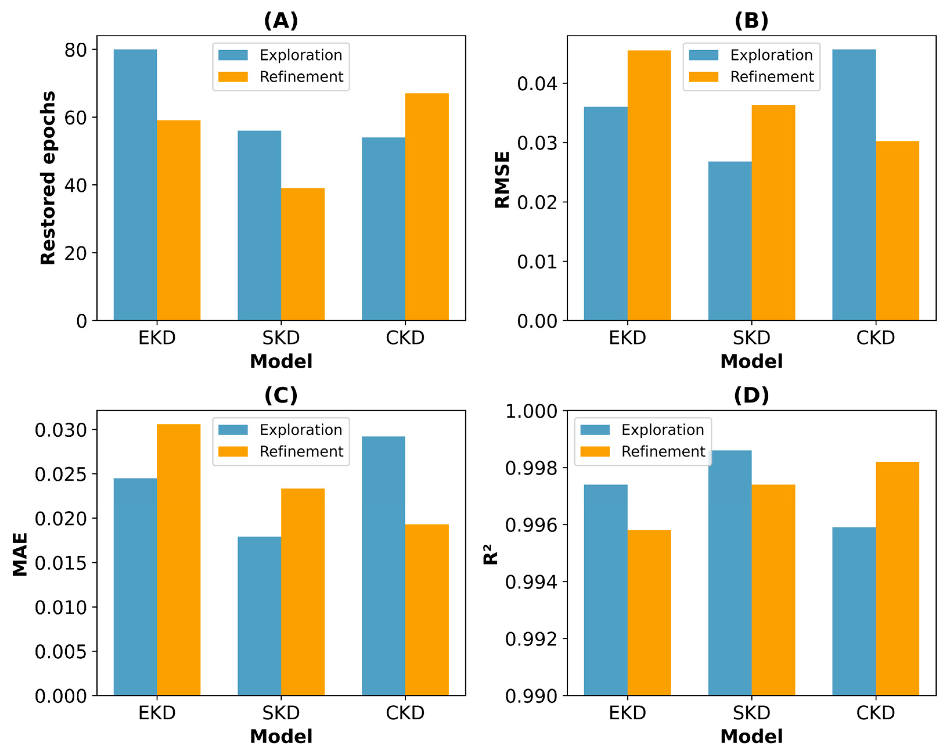
Implementing early stopping was crucial to preventing overfitting by terminating the training when the models did not improve further. Analyzing the restored epochs revealed distinct convergence patterns among the model types. The SKD-based models demonstrated the most efficient convergence, with mean values of 36.2 and 34.6 epochs for SKD1 and SKD2, respectively, reflecting their faster learning capabilities. This efficiency aligns with the 40-epoch limit established during the second optimization stage and suggests that the controlled nature of the synthetic dataset facilitates fast learning. In contrast, the EKD-based models required prolonged training, with mean values of 60.0 and 51.8 epochs for EKD1 and EKD2, reflecting the increased complexity inherent in the experimental data patterns. The CKD-based models exhibited intermediate behavior, with the mean number of restored epochs increasing from 39.4 in CKD1 to 54.8 in CKD2. This indicates that the refined hyperparameters in the second optimization stage required extended training to achieve optimal convergence with the heterogeneous combined dataset.

The models selected during the first optimization stage were initially constrained to 20 epochs; however, they were permitted to train for up to 60 epochs during cross-validation with early stopping. This additional training enabled first-stage models such as EKD1 to exceed the initially observed performance, thereby narrowing the performance gap between the optimization stages. Specifically, the EKD-based models exhibited a modest RMSE reduction from 0.0484 to 0.0458, whereas the CKD-based models improved from 0.0395 to 0.0303.

The SKD-based models performed better, with SKD1 achieving a mean RMSE of 0.0296 and SKD2 having a further reduced value of 0.0266. Similarly, the EKD and CKD models demonstrated improvements in the second optimization stage. The MAE followed a similar pattern, with SKD2 attaining the lowest MAE of 0.0186, underscoring its superior performance in minimizing prediction errors. All the models had high R² values exceeding 0.995. However, SKD2 had the highest value of 0.9986, indicating excellent explanatory capability.

The model stability was evaluated using the CoV of each performance metric, where lower CoV values signified greater stability and consistency in the model predictions. During the first optimization stage, CKD1 was the most stable, achieving the lowest CoV values for the RMSE (10.27%), MAE (11.25%), and R² (0.0602). Conversely, SKD1 had greater variability, particularly in CoV RMSE (28.38%) and MAE (30.84%). Higher CoV values for SKD1 may reflect suboptimal hyperparameter configurations, leading to overfitting. This overfitting could result in the model’s good performance metrics on average but with noticeable variability because it may have been overly sensitive to noise or specific patterns in the training data.

In the second optimization stage, all models had considerably reduced CoV, indicating enhanced stability. SKD2 achieved the lowest CoV across all metrics (RMSE: 6.41%, MAE: 8.54%, and R²: 0.0201%), underscoring the effectiveness of a more comprehensive hyperparameter tuning in stabilizing model performance. The EKD2 and CKD2 models also benefited from the reduced variability, with CoV RMSE values of 9.66% and 8.32%, respectively.

Higher CoV values in the first stage highlighted greater instability in model performance, likely caused by overfitting owing to suboptimal hyperparameter settings. This resulted in models that were overly sensitive to noise, leading to substantial variability across folds. The second optimization stage addressed these challenges through improved hyperparameter tuning and regularization techniques, reducing performance fluctuations. Consequently, the second-stage models achieved lower CoV values, reflecting enhanced stability, better generalization, and more reliable predictions.

3.3. The Performance of the Production Models

The production models were trained using 100% of the dataset for each variant once the hyperparameters were validated through cross-validation. The maximum number of training epochs for each production model was set as the mean number of epochs from the cross-validation phase plus one standard deviation. This strategy ensured a balanced approach between allowing sufficient training time for convergence and preventing excessive training, which could lead to overfitting.

Table 8. Performance metrics and epochs restored for final production models.

Model	Maximum Training Epochs	Epochs Restored	RMSE	MAE	R2
EKD1	88	80	0.0360	0.0245	0.9974
SKD1	56	56	0.0268	0.0179	0.9986
CKD1	54	54	0.0457	0.0292	0.9959
EKD2	65	59	0.0455	0.0306	0.9958
SKD2	39	39	0.0363	0.0233	0.9974
CKD2	67	67	0.0302	0.0193	0.9982

and Figure 4 indicate that the models achieved strong and consistent performances across all datasets. All models reached high R² values, exceeding 0.9958, confirming their ability to explain most of the data variance. The improvement in metrics compared with the cross-validation stage reflects the benefits of using the full dataset for training. This approach allows the models to capture more patterns and nuances in the data, thereby reducing variability and enhancing stability.

The results reveal that SKD1 achieved the best performance metrics, with the lowest RMSE (0.0268), MAE (0.0179), and R² (0.9986). This reinforces the advantages of synthetic datasets because their controlled and homogeneous nature yields stable and precise models. Among the combined datasets, CKD2 outperformed CKD1, achieving an RMSE of 0.0302, MAE of 0.0193, and R² of 0.9982. These results confirmed the effectiveness of the second-stage optimization and the ability of the models to capture complex patterns in the combined data.

Interestingly, the metrics (RMSE and MAE) of EKD1 and SKD1 were slightly better than those of their second-stage counterparts, EKD2 and SKD2. However, as observed in the k-fold cross-validation, these first-stage models were less stable, with higher CoV values. Overfitting tendencies in the first-stage models may explain this apparent contradiction. They excel in fitting the training data; however, they lack the robustness required for consistent generalization across various subsets of data. In contrast, the second-stage optimization likely promoted more generalized solutions by refining the hyperparameters, resulting in slightly higher RMSE and MAE values but improved stability. This trade-off was evident for synthetic data, where SKD1 had stronger metrics, whereas SKD2 had better balanced performance and reliability.

The number of epochs restored by early stopping also sheds light on the training. Based on the cross-validation results, the maximum epoch limit was effectively enforced across all the production models. Notably, the first-stage optimization models (EKD1 and SKD1) converged before reaching the maximum epoch limit, indicating that the training was sufficient for achieving optimal performance without unnecessary prolongation. In particular, the SKD2 model converged in 39 epochs and remained within the maximum limit of 39 epochs. Models trained on combined datasets, such as CKD1 (54 epochs) and CKD2 (67 epochs), required more epochs to achieve convergence, reflecting the inherent complexity and variability of the combined datasets compared with the synthetic ones. This suggests that combined datasets, which incorporate synthetic and experimental data, require more training time to achieve optimal performance, owing to their increased complexity and diversity.

3.4. Predictive Performance on Unseen Kinetic Profiles

Table 9. Metrics for predicting kinetic validation.

Validation Kinetic	Metric	EKD1	EKD2	SKD1	SKD2	CKD1	CKD2
Kinetic 1	RMSE	0.0450	0.0288	0.0181	0.0270	0.0302	0.0412
	R2	0.9771	0.9906	0.9963	0.9918	0.9897	0.9808
Kinetic 2	RMSE	0.0922	0.0952	0.1615	0.1657	0.1485	0.1340
	R2	0.9783	0.9769	0.9335	0.9300	0.9438	0.9542
Kinetic 3	RMSE	0.0382	0.0372	0.0618	0.0599	0.0616	0.0648
	R2	0.9774	0.9786	0.9410	0.9446	0.9415	0.9352
Kinetic 4	RMSE	0.0537	0.0409	0.0831	0.0567	0.0506	0.0896
	R2	0.9617	0.9779	0.9086	0.9574	0.9661	0.8937

and Figure 5 reveal that the generalization capabilities of the models were assessed using four unseen kinetics under varying conditions. These kinetics introduced various concentrations of Ni(II), temperatures, pH levels, and salts, thereby assessing the robustness and adaptability of the models.

For Kinetic 1 (Co_Ni(II) = 1.5 mM, T = 20 °C, pH = 8.0, without salt), Figure 5A–C revealed that all models demonstrated strong predictive performance, with RMSE values of 0.0181–0.0450 and R² values exceeding 0.977. The predicted curves generally maintained smooth trends that aligned closely with the experimental data. Among all the models, SKD1 achieved the lowest RMSE (0.0181) and the highest R² (0.9963), indicating superior accuracy in predicting biosorption kinetics under these conditions.

Under the more demanding Kinetic 2 conditions (Figure 5D–F), characterized by a higher Ni(II) concentration and an elevated temperature, the trained models were more robust. EKD1 and EKD2 outperformed the synthetic data-based models, with RMSE values of 0.0922 and 0.0952, respectively, compared to SKD1 (0.1615) and SKD2 (0.1657). All models displayed some abrupt changes during rapid transitions from high-velocity to plateau regions, which are inherent to the increased complexity at elevated temperatures and concentrations. This divergence highlights the importance of incorporating experimental data to capture the intricate system behaviors that synthetic models may struggle to replicate under such intensified conditions.

Introducing ionic effects in Kinetic 3 (Figure 5G–I) with NaCl addition further enabled the evaluation of the models’ adaptability. In this scenario, the experimental models demonstrated superior performance. EKD1 and EKD2 achieved the best results, with RMSE values of 0.0382 and 0.0372, respectively, and R² values of 0.9774 and 0.9786, respectively. The SKD models predicted lower values in the plateau region while maintaining smooth curves, indicating a tendency to underestimate the final biosorption capacity under ionic influence. The CKD1 and CKD2 models had average performances with RMSE values of 0.0616 and 0.0648, respectively.

In Kinetic 4 (Figure 5J–L), EKD2 performed best, with an RMSE of 0.0409 and R² of 0.9779, followed by EKD1 with an RMSE of 0.0537 and R² of 0.9617 in the presence of MgCl2. The synthetic data-based models and combined models exhibited inferior performance, with RMSE values of 0.0567–0.0896. MgCl₂ introduced additional ionic interactions that were challenging for synthetic models, highlighting the advantages of experimental data-based models for modeling complex biosorption kinetics.

Validation with unseen kinetics revealed differences in model performance. The synthetic data-based models excelled under simple conditions, such as kinetic 1, achieving the lowest RMSE and highest R² values. However, their accuracy decreased in more complex scenarios involving higher concentrations, elevated temperatures, and ionic interactions. In contrast, experimental data-based models demonstrated greater adaptability and accuracy under challenging conditions, outperforming the synthetic and combined models in kinetics 3 and 4, in which ionic effects were crucial. The combined models exhibited average performance, balancing the experimental and synthetic trends. Overall, the EKD models were more consistent, highlighting the importance of incorporating experimental data for real-world applications, particularly under specific ionic conditions.

3.5. Response Surface Analysis

The response surface analysis was conducted under some of the most challenging conditions in this study, involving complex parameter interactions and dynamic transitions that are inherently challenging to predict. The models demonstrated strong generalization capabilities in unseen kinetic validation, as indicated by their high R² values. However, the analysis of response surfaces provides an opportunity to evaluate their performance under conditions that may test the limits of the datasets used for training and validation. This analysis is relevant for identifying potential gaps in the ability of datasets to capture intricate adsorption dynamics across various operational parameters.

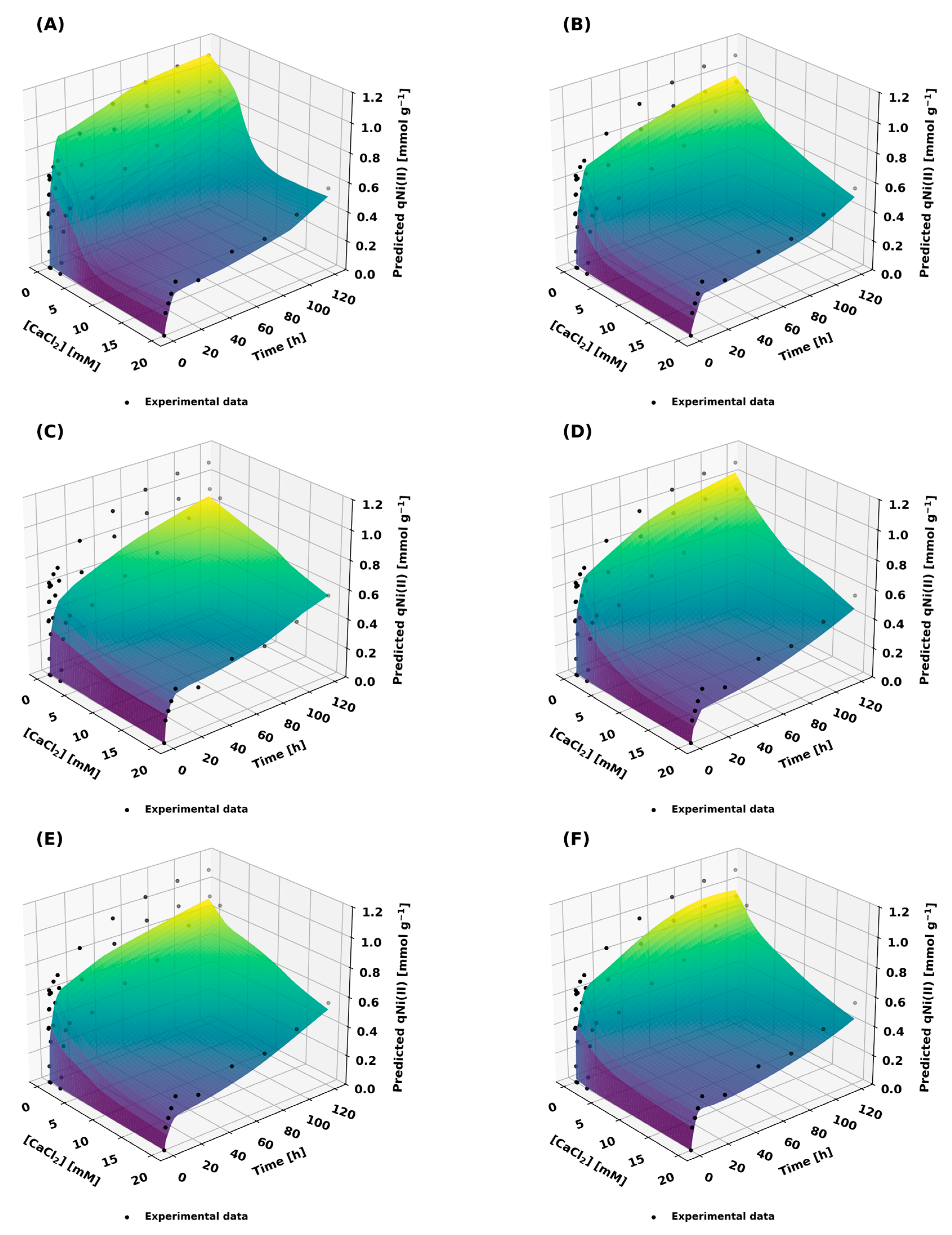
Figure 6 and Figure 7 illustrate the response surfaces of qNi(II) as a function of time and salt concentration for NaCl and CaCl₂, respectively. These figures allow for a detailed examination of the predictive behavior of the models and how effectively they represent the underlying adsorption phenomena under varying conditions. In addition, the evaluation metrics are summarized in

Table 10. Performance metrics for predicting biosorption experimental kinetic data in the presence of NaCl and CaCl₂.

Salt	Metric	EKD1	EKD2	SKD1	SKD2	CKD1	CKD2
NaCl	RMSE	0.0608	0.0887	0.0947	0.1004	0.0831	0.0814
	R2	0.9507	0.9159	0.9041	0.8924	0.9263	0.9292
CaCl2	RMSE	0.0882	0.1113	0.1233	0.1263	0.1091	0.1071
	R2	0.9154	0.8652	0.8346	0.8264	0.8705	0.8752

, providing a quantitative assessment of how well the models fit the experimental data.

Figure 6 illustrates the impact of NaCl concentration on adsorption. The experimental data-based models (Figure 6A,B) captured the general adsorption trends well at intermediate salt concentrations but showed deviations at low NaCl levels, indicating limitations in representing subtle adsorption dynamics. EKD1 achieved an R² of 0.9507, while EKD2 reached 0.9159. The synthetic data-based models (Figure 6C,D) provided smoother predictions across the entire range but lacked the accuracy to replicate localized transitions, with R² values of 0.9041 for SKD1 and 0.8924 for SKD2. The combined data models (Figure 6E,F) showed a more balanced performance, integrating the strengths of both datasets, with R² values of 0.9263 for CKD1 and 0.9292 for CKD2.

Figure 7 illustrates the adsorption behavior of CaCl₂ as an influencing factor. The EKD models (Figure 7A,B) demonstrated strong performance at intermediate and high salt concentrations; however, they struggled to capture trends at lower concentrations, consistent with the observations from Figure 6, EKD1 and EKD2 achieved R² values of 0.9154 and 0.8652, respectively. The synthetic data models (Figure 7C,D) produced generalized trends but lacked precision in the transition regions. The combined data models (Figure 7E,F) performed reasonably well, offering a compromise between the strengths and weaknesses of the individual datasets, with R² values of 0.8705 for CKD1 and 0.8752 for CKD2.

Validation results and response surface analysis demonstrated that the proposed methodology, including hyperparameter optimization and model selection, effectively captured the adsorption dynamics under diverse experimental conditions. The models exhibited strong generalization capabilities with high predictive accuracy in most scenarios. However, some of the observed limitations, particularly under more complex conditions, may be attributed to the characteristics of the datasets used for training and validation rather than deficiencies in the modeling approach. Addressing these dataset-related limitations can enhance model performance and applicability.

The EKD models provided the most accurate predictions under complex adsorption conditions, such as elevated ionic concentrations and temperature variations, as confirmed by unseen kinetic validation and response surface analyses. However, at lower ionic concentrations, deviations from the experimental behavior were observed, suggesting that these models perform optimally under intermediate conditions but may struggle at extremely low concentrations. Transitioning to strategic multivariate experimental designs would improve dataset diversity while minimizing the experimental effort. Combining this approach with active machine learning techniques such as Bayesian optimization can further refine experimental designs by identifying the most informative parameter regions [73].

The SKD models derived from synthetic datasets performed excellently under standard conditions, as evidenced by the strong metrics for simpler validation kinetics. However, their performance declined under more complex scenarios, such as higher concentrations, elevated temperatures, and the presence of salts. These limitations were also evident in the response surface analysis, in which the SKD models struggled to capture subtle transitions at low ionic concentrations. The incorporation of process variability and noise patterns into synthetic datasets can enhance their robustness in dynamic systems under diverse conditions. Advanced techniques, such as Copula Generative Adversarial Networks (CopulaGAN) and Total Variational Autoencoders (TVAE), offer promising solutions for improving synthetic data quality [74].

The CKD approach, which integrates experimental and synthetic datasets, offers a consistent performance by balancing the strengths of each data type. This integration reduces the limitations associated with the individual datasets, resulting in reliable predictions across various scenarios. However, the CKD models occasionally exhibited an intermediate performance between that of the SKD and EKD models. For instance, in the response surface analyses, CKD models provided reasonable predictions but lacked the precision of EKD models in capturing specific adsorption trends. Future research should focus on developing adaptive weighting schemes that dynamically adjust the contributions of synthetic and experimental data based on specific conditions.

3.6. SHAP Analysis

SHAP analysis provided key insights into the relative importance of the variables influencing the Ni(II) biosorption models.

Table 11. Relative importance of SHAP features on the models’ outputs.

Model	Time	Co Ni(II)	Salt Conc	T	pH	Salt Code	Cation Charge
EKD1	0.2825	0.1537	0.0914	0.0843	0.0644	0.0357	0.0297
EKD2	0.2440	0.1786	0.0708	0.0907	0.0525	0.0805	0.0408
SKD1	0.2653	0.1412	0.0593	0.0726	0.0667	0.1048	0.0617
SKD2	0.2915	0.2136	0.0737	0.1354	0.0693	0.0691	0.0567
CKD1	0.2694	0.1917	0.0538	0.1059	0.0699	0.0557	0.0444
CKD2	0.2731	0.1636	0.1061	0.0736	0.0480	0.0711	0.0477

highlights that time was consistently the most influential feature across all models, with relative importance values ranging from 0.2440 to 0.2915. Figure 8 reveals that longer contact times yielded predicted values above the baseline, reflecting the natural progression of biosorption toward equilibrium. This behavior is consistent with the equilibrium approach described by the pseudo-second-order kinetic model, which effectively describes the processes involved in Ni(II) biosorption [27].

The initial Ni(II) concentration was ranked as the second most influential factor, with predominantly positive contributions from SHAP. The SKD2 model demonstrated this feature to be the most important (0.2136), followed by the CKD1 (0.1917). The SHAP summary plots indicate that higher initial concentrations favor the adsorption capacity, consistent with mass transfer principles, where larger concentration gradients increase the driving force for adsorption [75].

Temperature and pH had variable but significant effects on biosorption. Temperature consistently exhibited a positive influence across all six models, indicating that higher temperatures enhanced adsorption capacity. The relative importance of temperature varied among the models; however, the overall trend remained clear, supporting its role in accelerating the adsorption kinetics, likely due to improved molecular interactions and increased diffusion rates in endothermic systems [18]. Similarly, higher pH values predominantly contributed positively to the SHAP analysis, suggesting that an increase in pH enhanced the adsorption capacity by modulating the functional groups of the biosorbent. These findings are consistent with previous studies on Ni(II) biosorption using various biological materials, where an endothermic process with optimal pH values above 7.0 has been reported [27,76,77].

Features related to the presence of salts, including salt concentration, salt code, and cation charge, were crucial in influencing model predictions and highlighting the complex interactions governing biosorption in saline environments. High salt concentrations consistently exhibited negative SHAP contributions across the models, with CKD2 exhibiting the most pronounced effect (0.1061). This confirms their adverse impact on the adsorption capacity of toxic metals, as previously reported for adsorption systems [78,79,80].

The salt code, introduced as a categorical variable (0–7), provides a practical yet generalized approach to representing complex ionic influences on qNi(II). This feature effectively captures the differential effects of various salts, even when the underlying mechanisms are not fully understood. Most models, including CKD2 and SKD1, successfully captured the expected trend, where higher values of the categorical feature salt code corresponded to more pronounced negative effects on the biosorption capacity. For instance, CKD2 and SKD1 assigned notable importance to this feature (0.0711 and 0.1048, respectively), leveraging their ability to encapsulate diverse salt-related interactions. However, EKD1 did not reproduce this trend, possibly because of the suboptimal hyperparameter selection or the challenge of capturing ionic interactions.

The salt code offers valuable insights; however, it has inherent limitations because it does not explicitly separate the effects of specific factors, such as the role of anions or structural differences among salts. Nonetheless, the advantage of using such models lies in their adaptability, which allows the incorporation of additional information that becomes available.

The cation charge demonstrated surprisingly low relative importance across all the models (0.0297–0.0617), and only the CKD1 model accurately captured the expected dominance of divalent cation competition. This model exhibited more pronounced negative SHAP contributions for divalent ions despite extensive literature documenting the stronger competitive effects of different valence states in biosorption systems involving divalent metals. Previous studies have suggested that under similar molar concentrations, divalent cations generally exhibit a higher tendency to compete for adsorption sites than monovalent ions [28,34]. This unexpected model behavior may be explained by the salt code feature implicitly incorporating valence effects along with other factors, leading to partial redundancy in the information captured. This limitation does not affect the overall predictive accuracy. Nonetheless, it suggests that the current feature engineering approach requires refinement, particularly in terms of differentiating the overlapping contributions of the salt code from cation charge variables.

The SHAP analysis highlighted the strengths of the current models and further refinement areas. Key variables, such as time and initial Ni(II) concentration, are well-represented; however, modeling ionic competition mechanisms requires improvement. The salt code provides a generalized view of ionic effects but overlaps with the cation charge variable, potentially obscuring specific competitive interactions.

Future work should focus on refining feature engineering to better capture these ionic interactions, possibly by splitting the salt code into distinct components that account for individual anionic and cationic influences or by incorporating more detailed measures of ionic strength and specific ion interactions. However, such refinements may also increase the model complexity and introduce additional uncertainties. Thus, proposed modifications must balance the improved representation with potential drawbacks, such as overfitting and higher computational demands.

While mechanistic models have been instrumental in advancing the fundamental understanding of biosorption processes—by providing insight into adsorption mechanisms, reaction kinetics, and thermodynamic behavior—they are limited when it comes to integrating multiple experimental variables or predicting system behavior under novel conditions. In contrast, the data-driven Bi-LSTM models developed in this study offer enhanced predictive capabilities that extend beyond descriptive modeling [81]. By learning directly from experimental and synthetic data, these models are able to capture complex, nonlinear interactions between environmental variables, such as salinity, pH, temperature, and initial metal concentration, which are often difficult to isolate or model mechanistically.

This transition from descriptive to predictive modeling represents a critical step toward practical implementation. In real or pilot-scale treatment systems, such models could assist in scenario simulation, process optimization, and even real-time decision-making by forecasting system behavior under fluctuating influent conditions [69,82,83]. Moreover, the ability to incorporate synthetic data into the training process presents an opportunity to reduce experimental load and cost, especially when working with hazardous materials or highly variable wastewater compositions. Ultimately, this approach contributes to bridging the gap between laboratory-scale research and scalable, adaptive biosorption technologies suitable for industrial applications.

4. Conclusions

The two-stage hyperparameter optimization achieved low RMSE values and R² values exceeding 0.995, demonstrating that systematic tuning is essential for improving the model performance. This process ensured that the Bi-LSTM networks remained efficient and stable across the diverse datasets.

Incorporating specialized features, such as the electrolyte cation charge and a novel salt code, was critical for capturing the intricate effects of coexisting salts. These enhancements improved the interpretability of the model in terms of ionic interactions, although further refinements are required to fully decouple the overlapping effects.

The Bi-LSTM network was highly effective in modeling Ni(II) biosorption kinetics in saline environments. Its ability to capture complex temporal dynamics provides a robust framework for understanding and predicting the dynamic behavior of biosorption processes.

Validation with unseen kinetics and response surface analysis provided valuable insights into how variations in salt concentration and operational parameters affect biosorption kinetics. These analyses confirmed the predictive accuracy of the model and offered practical guidance for optimizing biosorption under various conditions.

The SKD-based models exhibited superior performance under standard conditions and were characterized by faster convergence and lower prediction errors. The controlled nature of the synthetic data was highly beneficial for the initial model training and evaluation.

The models developed with EKD were more robust in complex scenarios, such as high temperatures and intricate ionic interactions, making them more representative of real-world variability.

The CKD models, which integrated synthetic and experimental data, achieved a balanced performance by combining the precision of synthetic data with the robustness of experimental measurements. This integration yielded reliable predictions across diverse conditions.

SHAP analysis consistently identified contact time and initial Ni(II) concentration as the most influential factors in predicting biosorption capacity. These findings reinforce the critical role of these variables and provide clear guidance for process optimization.

Despite these promising results, significant opportunities for future research remain. Adopting strategic multivariate experimental designs will be crucial to expand the diversity of experimental conditions, reduce bias, and enhance dataset representativeness. Additionally, refining synthetic data-generation methods is essential to better capture the variability and noise inherent in real-world biosorption processes across different metals. Further advancements in feature engineering could improve the modeling of complex ionic effects by developing new quantitative descriptors related to cation charge, ionic strength, and salt-specific properties. These refinements are expected to enhance the generalizability of the predictive models, ultimately leading to more robust and interpretable deep learning tools for optimizing biosorption across various heavy metals and environmental conditions.

References

1. Ajibade, F.O.; Adelodun, B.; Lasisi, K.H.; Fadare, O.O.; Ajibade, T.F.; Nwogwu, N.A.; Sulaymon, I.D.; Ugya, A.Y.; Wang, H.C.; Wang, A. Environmental pollution and their socioeconomic impacts. In Microbe Mediated Remediation of Environmental Contaminants; Kumar, A., Kumar Singh, V., Singh, P., Kumar Mishra, V., Eds.; Elsevier: Duxford, UK, 2021; pp. 321–354. [Google Scholar]
2. Lin, L.; Yang, H.; Xu, X. Effects of Water Pollution on Human Health and Disease Heterogeneity: A Review. Front. Environ. Sci. 2022, 10, 880246. [Google Scholar]
3. Jan, S.; Mishra, A.K.; Bhat, M.A.; Bhat, M.A.; Jan, A.T. Pollutants in aquatic system: A frontier perspective of emerging threat and strategies to solve the crisis for safe drinking water. Environ. Sci. Pollut. Res. 2023, 30, 113242–113279. [Google Scholar] [CrossRef]
4. Hublikar, L.V.; Shilar, F.A.; Suliphuldevara Mathada, B.; Ganachari, S.V. A comprehensive investigation of green solutions for sustainable wastewater remediation: A review. J. Mol. Liq. 2024, 400, 124532. [Google Scholar] [CrossRef]
5. Ahmed, M.; Mavukkandy, M.O.; Giwa, A.; Elektorowicz, M.; Katsou, E.; Khelifi, O.; Naddeo, V.; Hasan, S.W. Recent developments in hazardous pollutants removal from wastewater and water reuse within a circular economy. npj Clean Water 2022, 5, 12. [Google Scholar]
6. Oladimeji, T.E.; Oyedemi, M.; Emetere, M.E.; Agboola, O.; Adeoye, J.B.; Odunlami, O.A. Review on the impact of heavy metals from industrial wastewater effluent and removal technologies. Heliyon 2024, 10, e40370. [Google Scholar] [PubMed]
7. Razzak, S.A.; Faruque, M.O.; Alsheikh, Z.; Alsheikhmohamad, L.; Alkuroud, D.; Alfayez, A.; Hossain, S.Z.; Hossain, M.M. A comprehensive review on conventional and biological-driven heavy metals removal from industrial wastewater. Environ. Adv. 2022, 7, 100168. [Google Scholar]
8. Fulke, A.B.; Ratanpal, S.; Sonker, S. Understanding heavy metal toxicity: Implications on human health, marine ecosystems and bioremediation strategies. Mar. Pollut. Bull. 2024, 206, 116707. [Google Scholar] [CrossRef]
9. Dhokpande, S.R.; Deshmukh, S.M.; Khandekar, A.; Sankhe, A. A review outlook on methods for removal of heavy metal ions from wastewater. Sep. Purif. Technol. 2024, 350, 127868. [Google Scholar]
10. Begum, W.; Rai, S.; Banerjee, S.; Bhattacharjee, S.; Mondal, M.H.; Bhattarai, A.; Saha, B. A comprehensive review on the sources, essentiality and toxicological profile of nickel. RSC Adv. 2022, 12, 9139–9153. [Google Scholar] [CrossRef]
11. Kumar, A.; Jigyasu, D.K.; Kumar, A.; Subrahmanyam, G.; Mondal, R.; Shabnam, A.A.; Cabral-Pinto, M.M.S.; Malyan, S.K.; Chaturvedi, A.K.; Gupta, D.K.; et al. Nickel in terrestrial biota: Comprehensive review on contamination, toxicity, tolerance and its remediation approaches. Chemosphere 2021, 275, 129996. [Google Scholar]
12. Wang, Z.; Yeung, K.W.Y.; Zhou, G.J.; Yung, M.M.N.; Schlekat, C.E.; Garman, E.R.; Gissi, F.; Stauber, J.L.; Middleton, E.T.; Wang, Y.Y.L.; et al. Acute and chronic toxicity of nickel on freshwater and marine tropical aquatic organisms. Ecotox. Environ. Safe. 2020, 206, 111373. [Google Scholar] [CrossRef] [PubMed]
13. Das, K.K.; Reddy, R.C.; Bagoji, I.B.; Das, S.; Bagali, S.; Mullur, L.; Khodnapur, J.P.; Biradar, M.S. Primary concept of nickel toxicity—An overview. J Basic Clin. Physiol. Pharmacol. 2019, 30, 141–152. [Google Scholar] [CrossRef] [PubMed]
14. Genchi, G.; Carocci, A.; Lauria, G.; Sinicropi, M.S.; Catalano, A. Nickel: Human Health and Environmental Toxicology. Int. J. Environ. Res. Public Health 2020, 17, 679. [Google Scholar] [CrossRef] [PubMed]
15. Buxton, S.; Garman, E.; Heim, K.E.; Lyons-Darden, T.; Schlekat, C.E.; Taylor, M.D.; Oller, A.R. Concise Review of Nickel Human Health Toxicology and Ecotoxicology. Inorganics 2019, 7, 89. [Google Scholar] [CrossRef]
16. Macomber, L.; Hausinger, R.P. Mechanisms of nickel toxicity in microorganisms. Metallomics 2011, 3, 1153–1162. [Google Scholar] [CrossRef]
17. Yaashikaa, P.R.; Palanivelu, J.; Hemavathy, R.V. Sustainable approaches for removing toxic heavy metal from contaminated water: A comprehensive review of bioremediation and biosorption techniques. Chemosphere 2024, 357, 141933. [Google Scholar] [CrossRef]
18. Naja, G.; Volesky, B. The Mechanism of Metal Cation and Anion Biosorption. In Microbial Biosorption of Metals; Kotrba, P., Mackova, M., Macek, T., Eds.; Springer: Dordrecht, The Netherlands, 2011; pp. 19–58. [Google Scholar]
19. Elgarahy, A.M.; Elwakeel, K.Z.; Mohammad, S.H.; Elshoubaky, G.A. A critical review of biosorption of dyes, heavy metals and metalloids from wastewater as an efficient and green process. Clean. Eng. Technol. 2021, 4, 100209. [Google Scholar] [CrossRef]
20. Anastopoulos, I.; Pashalidis, I.; Hosseini-Bandegharaei, A.; Giannakoudakis, D.A.; Robalds, A.; Usman, M.; Escudero, L.B.; Zhou, Y.; Colmenares, J.C.; Núñez-Delgado, A.; et al. Agricultural biomass/waste as adsorbents for toxic metal decontamination of aqueous solutions. J. Mol. Liq. 2019, 295, 111684. [Google Scholar] [CrossRef]
21. Staszak, K.; Regel-Rosocka, M. Removing Heavy Metals: Cutting-Edge Strategies and Advancements in Biosorption Technology. Materials 2024, 17, 1155. [Google Scholar] [CrossRef]
22. Karnwal, A. Unveiling the promise of biosorption for heavy metal removal from water sources. Desalin. Water Treat. 2024, 319, 100523. [Google Scholar] [CrossRef]
23. Agarwal, A.; Upadhyay, U.; Sreedhar, I.; Singh, S.A.; Patel, C.M. A review on valorization of biomass in heavy metal removal from wastewater. J. Water Process Eng. 2020, 38, 101602. [Google Scholar]
24. Bădescu, I.S.; Bulgariu, D.; Ahmad, I.; Bulgariu, L. Valorisation possibilities of exhausted biosorbents loaded with metal ions—A review. J. Environ. Manage. 2018, 224, 288–297. [Google Scholar] [PubMed]
25. Abdolali, A.; Guo, W.S.; Ngo, H.H.; Chen, S.S.; Nguyen, N.C.; Tung, K.L. Typical lignocellulosic wastes and by-products for biosorption process in water and wastewater treatment: A critical review. Bioresour. Technol. 2014, 160, 57–66. [Google Scholar]
26. Tovar-Sánchez, E.; Oyama, K. Natural hybridization and hybrid zones between Quercus crassifolia and Quercus crassipes (Fagaceae) in Mexico: Morphological and molecular evidence. Am. J. Bot. 2004, 91, 1352–1363. [Google Scholar] [CrossRef] [PubMed]
27. Aranda-García, E.; Cristiani-Urbina, E. Kinetic, Equilibrium, and Thermodynamic Analyses of Ni(II) Biosorption from Aqueous Solution by Acorn Shell of Quercus crassipes. Water Air Soil Pollut. 2018, 229, 119. [Google Scholar]
28. Aranda-García, E.; Chávez-Camarillo, G.M.; Cristiani-Urbina, E. Effect of Ionic Strength and Coexisting Ions on the Biosorption of Divalent Nickel by the Acorn Shell of the Oak Quercus crassipes Humb. & Bonpl. Processes 2020, 8, 1229. [Google Scholar] [CrossRef]
29. Aranda-García, E.; Cristiani-Urbina, E. Hexavalent chromium removal and total chromium biosorption from aqueous solution by Quercus crassipes acorn shell in a continuous up-flow fixed-bed column: Influencing parameters, kinetics, and mechanism. PLoS ONE 2020, 15, e0227953. [Google Scholar]
30. Aranda-García, E.; Morales-Barrera, L.; Pineda-Camacho, G.; Cristiani-Urbina, E. Effect of pH, ionic strength, and background electrolytes on Cr(VI) and total chromium removal by acorn shell of Quercus crassipes Humb. & Bonpl. Environ. Monit. Assess. 2014, 186, 6207–6221. [Google Scholar]
31. Vijayaraghavan, K.; Balasubramanian, R. Is biosorption suitable for decontamination of metal-bearing wastewaters? A critical review on the state-of-the-art of biosorption processes and future directions. J. Environ. Manage. 2015, 160, 283–296. [Google Scholar]
32. Guo, L.; Xie, Y.; Sun, W.; Xu, Y.; Sun, Y. Research Progress of High-Salinity Wastewater Treatment Technology. Water 2023, 15, 684. [Google Scholar] [CrossRef]
33. Zhang, Y.; Zhu, C.; Liu, F.; Yuan, Y.; Wu, H.; Li, A. Effects of ionic strength on removal of toxic pollutants from aqueous media with multifarious adsorbents: A review. Sci. Total Environ. 2019, 646, 265–279. [Google Scholar] [CrossRef]
34. Schiewer, S.; Volesky, B. Ionic Strength and Electrostatic Effects in Biosorption of Divalent Metal Ions and Protons. Environ. Sci. Technol. 1997, 31, 2478–2485. [Google Scholar] [CrossRef]
35. Ams, D.A.; Swanson, J.S.; Szymanowski, J.E.S.; Fein, J.B.; Richmann, M.; Reed, D.T. The effect of high ionic strength on neptunium (V) adsorption to a halophilic bacterium. Geochim. Cosmochim. Acta 2013, 110, 45–57. [Google Scholar] [CrossRef]
36. Wang, H.S.H.; Yao, Y. Machine learning for sustainable development and applications of biomass and biomass-derived carbonaceous materials in water and agricultural systems: A review. Resour. Conserv. Recycl. 2023, 190, 106847. [Google Scholar] [CrossRef]
37. Taoufik, N.; Boumya, W.; Achak, M.; Chennouk, H.; Dewil, R.; Barka, N. The state of art on the prediction of efficiency and modeling of the processes of pollutants removal based on machine learning. Sci. Total Environ. 2022, 807, 150554. [Google Scholar] [CrossRef]
38. Hafsa, N.; Rushd, S.; Al-Yaari, M.; Rahman, M. A Generalized Method for Modeling the Adsorption of Heavy Metals with Machine Learning Algorithms. Water 2020, 12, 3490. [Google Scholar] [CrossRef]
39. Fiyadh, S.S.; Alardhi, S.M.; Al Omar, M.; Aljumaily, M.M.; Al Saadi, M.A.; Fayaed, S.S.; Ahmed, S.N.; Salman, A.D.; Abdalsalm, A.H.; Jabbar, N.M.; et al. A comprehensive review on modelling the adsorption process for heavy metal removal from waste water using artificial neural network technique. Heliyon 2023, 9, e15455. [Google Scholar] [CrossRef]
40. Bhagat, S.K.; Tung, T.M.; Yaseen, Z.M. Development of artificial intelligence for modeling wastewater heavy metal removal: State of the art, application assessment and possible future research. J. Clean. Prod. 2020, 250, 119473. [Google Scholar] [CrossRef]
41. Elsayed, A.; Moussa, Z.; Alrdahe, S.S.; Alharbi, M.M.; Ghoniem, A.A.; El-khateeb, A.Y.; Saber, W.I.A. Optimization of Heavy Metals Biosorption via Artificial Neural Network: A Case Study of Cobalt (II) Sorption by Pseudomonas alcaliphila NEWG-2. Front. Microbiol. 2022, 13, 893603. [Google Scholar] [CrossRef]
42. Skrobek, D.; Krzywanski, J.; Sosnowski, M.; Kulakowska, A.; Zylka, A.; Grabowska, K.; Ciesielska, K.; Nowak, W. Prediction of Sorption Processes Using the Deep Learning Methods (Long Short-Term Memory). Energies 2020, 13, 6601. [Google Scholar] [CrossRef]
43. Yu, Y.; Si, X.; Hu, C.; Zhang, J. A Review of Recurrent Neural Networks: LSTM Cells and Network Architectures. Neural Comput. 2019, 31, 1235–1270. [Google Scholar] [PubMed]
44. Cruz-Victoria, J.C.; Netzahuatl-Muñoz, A.R.; Cristiani-Urbina, E. Long Short-Term Memory and Bidirectional Long Short-Term Memory Modeling and Prediction of Hexavalent and Total Chromium Removal Capacity Kinetics of Cupressus lusitanica Bark. Sustainability 2024, 16, 2874. [Google Scholar] [CrossRef]
45. Fawzy, M.; Nasr, M.; Adel, S.; Nagy, H.; Helmi, S. Environmental approach and artificial intelligence for Ni(II) and Cd(II) biosorption from aqueous solution using Typha domingensis biomass. Ecol. Eng. 2016, 95, 743–752. [Google Scholar] [CrossRef]
46. Dashti, A.; Raji, M.; Riasat Harami, H.; Zhou, J.L.; Asghari, M. Biochar performance evaluation for heavy metals removal from industrial wastewater based on machine learning: Application for environmental protection. Sep. Purif. Technol. 2023, 12, 123399. [Google Scholar]
47. Zhu, X.; Wang, X.; Ok, Y.S. The application of machine learning methods for prediction of metal sorption onto biochars. J. Hazard. Mater. 2019, 378, 120727. [Google Scholar] [CrossRef]
48. Fritsch, F.N.; Butland, J. A Method for Constructing Local Monotone Piecewise Cubic Interpolants. SIAM J. Sci. Stat. Comput. 1984, 5, 300–304. [Google Scholar] [CrossRef]
49. Zaghiyan, M.R.; Eslamian, S.; Gohari, A.; Ebrahimi, M.S. Temporal correction of irregular observed intervals of groundwater level series using interpolation techniques. Theor. Appl. Climatol. 2021, 145, 1027–1037. [Google Scholar]
50. Benchekroun, M.; Chevallier, B.; Zalc, V.; Istrate, D.; Lenne, D.; Vera, N. The Impact of Missing Data on Heart Rate Variability Features: A Comparative Study of Interpolation Methods for Ambulatory Health Monitoring. Innov. Res. BioMed. Eng. (IRBM) 2023, 44, 100776. [Google Scholar] [CrossRef]
51. Antary, N.; Trauth, M.H.; Marwan, N. Interpolation and sampling effects on recurrence quantification measures. Chaos 2023, 33, 103105. [Google Scholar]
52. Giuffrè, M.; Shung, D.L. Harnessing the power of synthetic data in healthcare: Innovation, application, and privacy. NPJ Digit. Med. 2023, 6, 186. [Google Scholar]
53. Alom, M.Z.; Taha, T.M.; Yakopcic, C.; Westberg, S.; Sidike, P.; Nasrin, M.S.; Hasan, M.; Van Essen, B.C.; Awwal, A.A.; Asari, V.K. A State-of-the-Art Survey on Deep Learning Theory and Architectures. Electronics 2019, 8, 292. [Google Scholar] [CrossRef]
54. Watanabe, S. Tree-Structured Parzen Estimator: Understanding Its Algorithm Components and Their Roles for Better Empirical Performance. arXiv 2023, arXiv:2304.11127v3. [Google Scholar]
55. Yang, L.; Shami, A. On hyperparameter optimization of machine learning algorithms: Theory and practice. Neurocomputing 2020, 415, 295–316. [Google Scholar] [CrossRef]
56. Akiba, T.; Sano, S.; Yanase, T.; Ohta, T.; Koyama, M. Optuna: A Next-generation Hyperparameter Optimization Framework. In Proceedings of the 25th ACM SIGKDD International Conference on Knowledge Discovery & Data Mining, Anchorage, AK, USA, 4–8 August 2019; pp. 2623–2631. [Google Scholar]
57. Wu, J.; Chen, X.Y.; Zhang, H.; Xiong, L.D.; Lei, H.; Deng, S.H. Hyperparameter Optimization for Machine Learning Models Based on Bayesian Optimization. J. Electron. Sci. Technol. 2019, 17, 26–40. [Google Scholar]
58. Clevert, D.A.; Unterthiner, T.; Hochreiter, S. Fast and Accurate Deep Network Learning by Exponential Linear Units (ELUs). arXiv 2016, arXiv:1511.07289v5. [Google Scholar]
59. Gal, Y.; Ghahramani, Z. A Theoretically Grounded Application of Dropout in Recurrent Neural Networks. arXiv 2016, arXiv:1512.05287v5. [Google Scholar]
60. Hanifi, S.; Cammarono, A.; Zare-Behtash, H. Advanced hyperparameter optimization of deep learning models for wind power prediction. Renew. Energy 2024, 221, 119700. [Google Scholar] [CrossRef]
61. Hochreiter, S.; Schmidhuber, J. Long Short-Term Memory. Neural Comput. 1997, 9, 1735–1780. [Google Scholar]
62. Wang, S.; Ma, C.; Xu, Y.; Wang, J.; Wu, W. A Hyperparameter Optimization Algorithm for the LSTM Temperature Prediction Model in Data Center. Sci. Program. 2022, 2022, 6519909. [Google Scholar] [CrossRef]
63. Dubey, S.R.; Singh, S.K.; Chaudhuri, B.B. Activation Functions in Deep Learning: A Comprehensive Survey and Benchmark. arXiv 2022, arXiv:2109.14545v3. [Google Scholar] [CrossRef]
64. Chai, M.; Xia, F.; Hao, S.; Peng, D.; Cui, C.; Liu, W. PV Power Prediction Based on LSTM with Adaptive Hyperparameter Adjustment. IEEE Access 2019, 7, 115473–115486. [Google Scholar] [CrossRef]
65. Masters, D.; Luschi, C. Revisiting Small Batch Training for Deep Neural Networks. arXiv 2018, arXiv:1804.07612v1. [Google Scholar]
66. Murphy, K.P. Machine Learning: A Probabilistic Perspective; MIT Press: Cambridge, MA, USA, 2014; p. 1098. [Google Scholar]
67. Normawati, D.; Ismi, D.P. K-Fold Cross Validation for Selection of Cardiovascular Disease Diagnosis Features by Applying Rule-Based Datamining. Simple 2019, 1, 62–72. [Google Scholar] [CrossRef]
68. Yates, L.A.; Aandahl, Z.; Richards, S.A.; Brook, B.W. Cross validation for model selection: A review with examples from ecology. Ecol. Monogr. 2022, 93, e1557. [Google Scholar] [CrossRef]
69. Alvi, M.; Batstone, D.; Mbamba, C.K.; Keymer, P.; French, T.; Ward, A.; Dwyer, J.; Cardell-Oliver, R. Deep learning in wastewater treatment: A critical review. Water Res. 2023, 245, 120518. [Google Scholar] [CrossRef]
70. Lundberg, S.M.; Lee, S.I. A Unified Approach to Interpreting Model Predictions. In Proceedings of the 31st International Conference on Neural Information Processing Systems, NIPS’17 Conference, Long Beach, CA, USA, 4–9 December 2017; pp. 4768–4777. [Google Scholar]
71. Hinton, G.E.; Srivastava, N.; Krizhevsky, A.; Sutskever, I.; Salakhutdinov, R.R. Improving neural networks by preventing co-adaptation of feature detectors. arXiv 2012, arXiv:1207.0580v1. [Google Scholar]
72. Srivastava, N.; Hinton, G.; Krizhevsky, A.; Sutskever, I.; Salakhutdinov, R. Dropout: A Simple Way to Prevent Neural Networks from Overfitting. J. Mach. Learn. Res. 2014, 15, 1929–1958. [Google Scholar]
73. Eyke, N.S.; Green, W.H.; Jensen, K.F. Iterative experimental design based on active machine learning reduces the experimental burden associated with reaction screening. React. Chem. Eng. 2020, 5, 1963–1972. [Google Scholar] [CrossRef]
74. Chia, M.Y.; Koo, C.H.; Huang, Y.F.; Di Chan, W.; Pang, J.Y. Artificial Intelligence Generated Synthetic Datasets as the Remedy for Data Scarcity in Water Quality Index Estimation. Water Resour. Manag. 2023, 37, 6183–6198. [Google Scholar] [CrossRef]
75. Basu, A.; Ali, S.S.; Hossain, S.S.; Asif, M. A Review of the Dynamic Mathematical Modeling of Heavy Metal Removal with the Biosorption Process. Processes 2022, 10, 1154. [Google Scholar] [CrossRef]
76. Barquilha, C.E.R.; Cossich, E.S.; Tavares, C.R.G.; Da Silva, E.A. Biosorption of nickel(II) and copper(II) ions from synthetic and real effluents by alginate-based biosorbent produced from seaweed Sargassum sp. Environ. Sci. Pollut. Res. 2019, 26, 11100–11112. [Google Scholar] [CrossRef]
77. Suazo-Madrid, A.; Morales-Barrera, L.; Aranda-García, E.; Cristiani-Urbina, E. Nickel(II) biosorption by Rhodotorula glutinis. J. Ind. Microbiol. Biotechnol. 2011, 38, 51–64. [Google Scholar]
78. Kasbaji, M.; Mennani, M.; Grimi, N.; Barba, F.J.; Oubenali, M.; Simirgiotis, M.J.; Mbarki, M.; Moubarik, A. Implementation and physico-chemical characterization of new alkali-modified bio-sorbents for cadmium removal from industrial discharges: Adsorption isotherms and kinetic approaches. Process Biochem. 2022, 120, 213–226. [Google Scholar]
79. Michalak, I.; Saeid, A.; Chojnacka, K. The effect of increase in concentration of Na(I) ions on biosorption of Cr(III) ions by Enteromorpha prolifera and Spirulina sp. Cent. Eur. J. Chem. 2013, 11, 313–319. [Google Scholar] [CrossRef]
80. Lach, J.; Okoniewska, E. Adsorption of Chromium and Nickel Ions on Commercial Activated Carbon—An Analysis of Adsorption Kinetics and Statics. Molecules 2023, 28, 7413. [Google Scholar] [CrossRef] [PubMed]
81. Witek-Krowiak, A.; Chojnacka, K.; Podstawczyk, D.; Dawiec, A.; Bubała, K. Application of response surface methodology and artificial neural network methods in modelling and optimization of biosorption process. Bioresour. Technol. 2014, 160, 150–160. [Google Scholar]
82. Lowe, M.; Qin, R.; Mao, X. A Review on Machine Learning, Artificial Intelligence, and Smart Technology in Water Treatment and Monitoring. Water 2022, 14, 1384. [Google Scholar] [CrossRef]
83. Imen, S.; Croll, H.C.; McLellan, N.L.; Bartlett, M.; Lehman, G.; Jacangelo, J.G. Application of machine learning at wastewater treatment facilities: A review of the science, challenges and barriers by level of implementation. Environ. Technol. Rev. 2023, 12, 493–516. [Google Scholar]
Figure 1. Methodological workflow for modeling Ni(II) biosorption kinetics.
Processes 13 01076 g001
Figure 2. Performance metrics of optimized Bi-LSTM models evaluated through k-fold cross-validation. (A) Restored epochs, (B) RMSE, (C) MAE, and (D) R2. Exploration stage models: EKD1, SKD1, and CKD1. Refinement stage models: EKD2, SKD2, and CKD2.
Processes 13 01076 g002
Figure 3. Coefficients of variation of optimized Bi-LSTM models evaluated through k-fold cross-validation. (A) RMSE, (B) MAE, and (C) R2. Exploration stage models: EKD1, SKD1, and CKD1. Refinement stage models: EKD2, SKD2, and CKD2.
Processes 13 01076 g003
Figure 4. Performance metrics of optimized Bi-LSTM production models for kinetic Ni(II) biosorption. (A) Restored epochs, (B) RMSE, (C) MAE, and (D) R2. Exploration stage models: EKD1, SKD1, and CKD1. Refinement stage models: EKD2, SKD2, and CKD2.
Processes 13 01076 g004
Figure 5. Comparison of the model predictions with experimental data for unseen validation kinetics. (AC) Kinetic 1: Co Ni(II) = 1.5 mM, T = 20 °C, pH = 8.0, without salt; (DF) Kinetic 2: Co Ni(II) = 3.9 mM, T = 40 °C, pH = 8.0, without salt; (GI) Kinetic 3: Co Ni(II) = 1.97 mM, T = 20 °C, pH = 8.0, with NaCl at 20 mM; and (JL) Kinetic 4: Co Ni(II) = 1.97 mM, T = 20 °C, pH = 8.0, with MgCl2 at 2 mM.
Processes 13 01076 g005
Figure 6. Surface response for qNi(II) as a function of NaCl concentration and time for EKD1 (A), EKD2 (B), SKD1 (C), SKD2 (D), CKD1 (E), and CKD2 (F) models. Conditions: Co Ni(II) = 1.97 mM, pH = 8, T = 20 °C.
Processes 13 01076 g006
Figure 7. Surface response for qNi(II) as a function of CaCl2 concentration and time for EKD1 (A), EKD2 (B), SKD1 (C), SKD2 (D), CKD1 (E), and CKD2 (F) models. Conditions: Co Ni(II) = 1.97 mM, pH = 8, T = 20 °C.
Processes 13 01076 g007
Figure 8. SHAP summary plot revealing the impact of different features on model predictions for EKD1 (A), EKD2 (B), SKD1 (C), SKD2 (D), CKD1 (E), and CKD2 (F) models. Baseline: Average of qNi(II) values.
Processes 13 01076 g008