Abstract
An integrated dynamic analysis and prediction method for shale gas reservoirs based on wellbore coupling has been developed, focusing on optimizing well production. This method integrates a three-dimensional geological model, a mechanical model, simulations of fracture propagation, and a numerical simulation in a gas reservoir to establish a continuous-flow model that links the gas reservoir, fractures, and wellbore after hydraulic fracturing. It enables comprehensive integrated production dynamic analysis and predictions. The process begins by trajectory modeling and attribute assignment. Subsequently, based on the regional tectonic map, contour lines are drawn, regional tectonic surfaces are established, segmentation and clustering are performed, and appropriate fracturing fluids and proppants are selected to simulate fracture network expansion. Finally, the integrated dynamic simulation model of the gas reservoir and wellbore is constructed using the Petrel RE module, considering the combined effects of wellbore flow and reservoir seepage. The model was developed from a single well and through three-dimensional geological modeling, the simulation of fracture propagation in hydraulic fracturing, and a numerical simulation. An integrated dynamic licensing and prediction methodology was established for a shale gas integration model with wellbore-gas reservoir coupling. Additionally, this study analyzes and establishes the optimal pressurization timing and regime for the pressurizer to enhance gas well production. The model was successfully applied for historical matching and dynamic predictions in a block in the southern Sichuan region, producing results closely aligned with the actual data, thus providing a robust tool for predicting the future production profiles of shale gas wells.
1. Introduction
As an important replacement resource for the global energy structure transformation, shale gas depends on the dynamic optimization of the whole life-cycle production system for its efficient development. In the early stage of development, gas wells can achieve high production by relying on natural formation energy, but the extremely low permeability of shale reservoirs leads to the exponential decay of wellhead pressure; most of the time, it is in a low-pressure production state [1,2,3,4]. The wellhead pressure is high at the beginning of shale gas extraction [5,6,7,8,9], but the pressure decays rapidly over a short period of time, and then, most of the time thereafter, the well is in a low-pressure production state. When the tubing pressure of the gas well approaches the gathering pipeline network pressure, the daily gas production of the gas well continues to decline; then, when the daily gas production is reduced to an economic limit of production, it is no longer economically efficient to continue production, so it is necessary to pressurize the gas well for further extraction [10,11]. When shale gas wells are exploited, it is necessary to make full use of the higher initial pressure for the exploitation of new shale gas wells, and it is also necessary to deal with the situation of the low-pressure production of gas wells that are put into production at an early stage [12,13]. Therefore, determining the pressurization timing and parameter optimization of shale gas wells is of great significance for the stable production of shale gas fields [14,15,16]. In 2017, Drouven et al. proposed a nonconvex mixed-integer nonlinear programming model, which is used to optimize the pressurization location of shale gas surface-gathering pipeline networks [17]. In 2021, BY Hong et al. proposed a method for determining the planning of equipment use in shale gas fields and developed an optimization model to help pressurizers determine the most cost-effective pressurization period [18]. In 2022, Chen Zhen et al. optimized the axial system structure of the compressor ground based on the response surface method, which effectively improved the extraction efficiency of shale gas [19]. In 2022, Zhou Jun et al. calculated the appropriate pressurization location and compressor cost based on the established mixed-integer nonlinear programming model [20]. In 2023, Kunyi Wu et al. considered the modularization of compressors and established a mixed-integer nonlinear programming (MINLP) model. This model is beneficial for the selection of pressurization locations and timings and can effectively address the utilization rate of compressors in the shale gas production process [21]. In 2024, Chen SQ et al. optimized the pressurization process in order to improve efficiency and reduce energy consumption [22]. In 2024, Chen DX et al. proposed a data-driven prediction model combining principal component analysis (PCA), particle swarm optimization (PSO) and long short-term memory (LSTM) to determine the acquisition of pressurization timing [23].
Although scholars have carried out many studies on the optimization of pressurization timing and the parameters of compressors during shale gas extraction, the current studies only consider the influence of the wellbore flow and fail to make effective use of the field measurement data, so the optimization of pressurization timing and the parameters of pressurizers is not always accurate. On this basis, this study couples the gas wellbore and the gas reservoir, establishing a shale gas integration model with wellbore–gas reservoir coupling, and selects the optimal pressurization timing and pressurization regime by making a dynamic prediction of the gas reservoir.
2. Overview of the Study Block
The South Sichuan tectonic belongs to the low-steep fold belt in southwest Sichuan in the central Sichuan uplift area, adjacent to the low fold belt of Nanjiang in Anyue in the east and northeast. It is connected to the Ziliujing depression tectonic group with the Xindianzi syncline in the south, facing the Longquanshan tectonic belt in the north and west boundaries of the Jinhe syncline and the Shoubaochang tectonic saddle in the southwest. The ground tectonics of the gas well area in the South Sichuan area under study are relatively gentle and simple in form, and no faults are seen; the faults at the bottom of the Upper Permian and the bottom of the Cambrian system in the Earth’s belly are relatively well developed, and the local development of orthogonal faults is relatively small in scale. The trend of the faults in the three-dimensional block is essentially nearly east–west and north–east. The main body of the tectonic structure of the South Sichuan block is north-east oriented, with a gentle dip, and the dip of the Longmaxi Formation gradually decreases from the north-west to the south-east, which is a relatively tectonically gentle area and is favorable for the preservation of shale gas.
3. Establishment of Shale Gas Wellbore Gas Reservoir Analysis Methods
There are three classical gas reservoir analysis methods: the decreasing capacity prediction method, the gas well inflow dynamic analysis method, and the numerical simulation for gas reservoirs method [24,25,26]. Considering that shale gas pressurization engineering operations bring about complex changes in reservoir seepage and wellbore flow, based on a comparison of the advantages and disadvantages of the three methods (Table 1), the gas reservoir numerical simulation method takes more influencing factors into consideration and is more suitable for analyzing the changes in gas well production dynamics brought about by pressurization operations. However, in conventional gas reservoir numerical simulations, most of the input fracture parameters are equivalent fracture patterns or regular fracture networks, which are detached from the real results of fracture expansion simulations. Moreover, the reservoir physical property parameters are modified during historical matching, and the transformation of physical properties not only causes changes in production but also affects the fracturing effect at the same time, which in turn affects the production capacity. Large-scale hydraulic fracturing brings about many difficulties in the optimization of shale gas development strategies, meaning that attention must be paid to both reservoir geology and the drilling and completion quality. Therefore, we also need to consider the impact caused by the hydraulic fracturing network. The optimization objectives of conventional hydraulic fracturing simulations are to optimize the fracture length, inflow capacity, and reformed zone scope, and the optimization indexes are controlled by the construction parameters, such as fluid strength, sand strength, displacement, and cluster spacing, etc. The optimal fracture reformed size is calculated via a fracturing simulation, but it is not possible to combine the geological attributes with the direct calculation of the production capacity of the gas wells [27,28,29].

Table 1.
Comparison of advantages and disadvantages of the three analysis methods.
As a result, both conventional numerical simulations and fracturing simulations suffer from inaccuracies in the input and output parameters. To resolve this relationship, it is necessary to carry out a complete process of simulation from geology to engineering to gas reservoir.
In this study, a shale gas integration model with wellbore–gas reservoir coupling is proposed after comparing the advantages and disadvantages of various dynamic analysis and prediction methods, addressing the interface and compatibility of geological modeling, fracturing extension simulation, and numerical simulation of the gas reservoir. The model is an integrated simulation method that combines geological attributes and geological modeling, fracture extension simulations, and gas reservoir numerical simulations. The method takes the production as the target, adopts the injection and fracturing construction parameters as the optimization indexes, and corrects each for the established integrated wellbore–gas reservoir coupling model, to realize integrated optimization.
4. Establishment of an Integrated Wellbore–Gas Reservoir Coupling Model
4.1. Establishment of a Three-Dimensional Structural Model and Property Model
(1) Before geological modeling, it is necessary to carry out the collection and preprocessing of raw formation data. This modeling study focuses on the South Sichuan block, targeting 13 shale gas wells in the region, to conduct an integrated wellbore–gas reservoir coupling model experiment. The required basic data for modeling include the wellhead coordinates, well trajectory data, logging interpretations, stratigraphic data, fracturing data, production data, and completion information for each well in the study block.
(2) Based on the collected and preprocessed data, geological structural models, property models, and in situ stress models were established for the 13 wells in the study block [30]. The well area boundaries and wellhead coordinates were determined, and the well trajectory data and logging interpretation structures were imported. Combining the logging data and interpretation results from wells in the South Sichuan block areas, one-dimensional property models along the wellbore were established. For the 13 producing wells, porosity ranges from 0.034 to 0.065, water saturation ranges from 0.32 to 0.51, minimum horizontal principal stress ranges from 85.3 to 91.7 MPa, maximum horizontal principal stress ranges from 97.4 to 107.4 MPa, and the average difference between the horizontal principal stresses is approximately 12 MPa.
(3) The geological structural map of the target well area was imported, and structural lines were drawn along the contour lines. The boundary range was selected to generate the structural surface. Based on the stratigraphic data of each well, the structural surface was divided into Long114, Long113, Long112, Long111, and the Wufeng Formation, and the distances between layers were set according to the given data. Based on the results of the stratigraphic testing and the drilling encounter rate of each well, the trend of the structural surface was adjusted to complete the three-dimensional structural model from the Wufeng Formation to the Long114 layer (Figure 1).
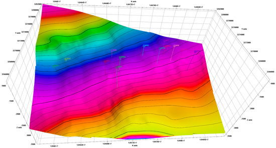
Figure 1.
Three−dimensional tectonic model.
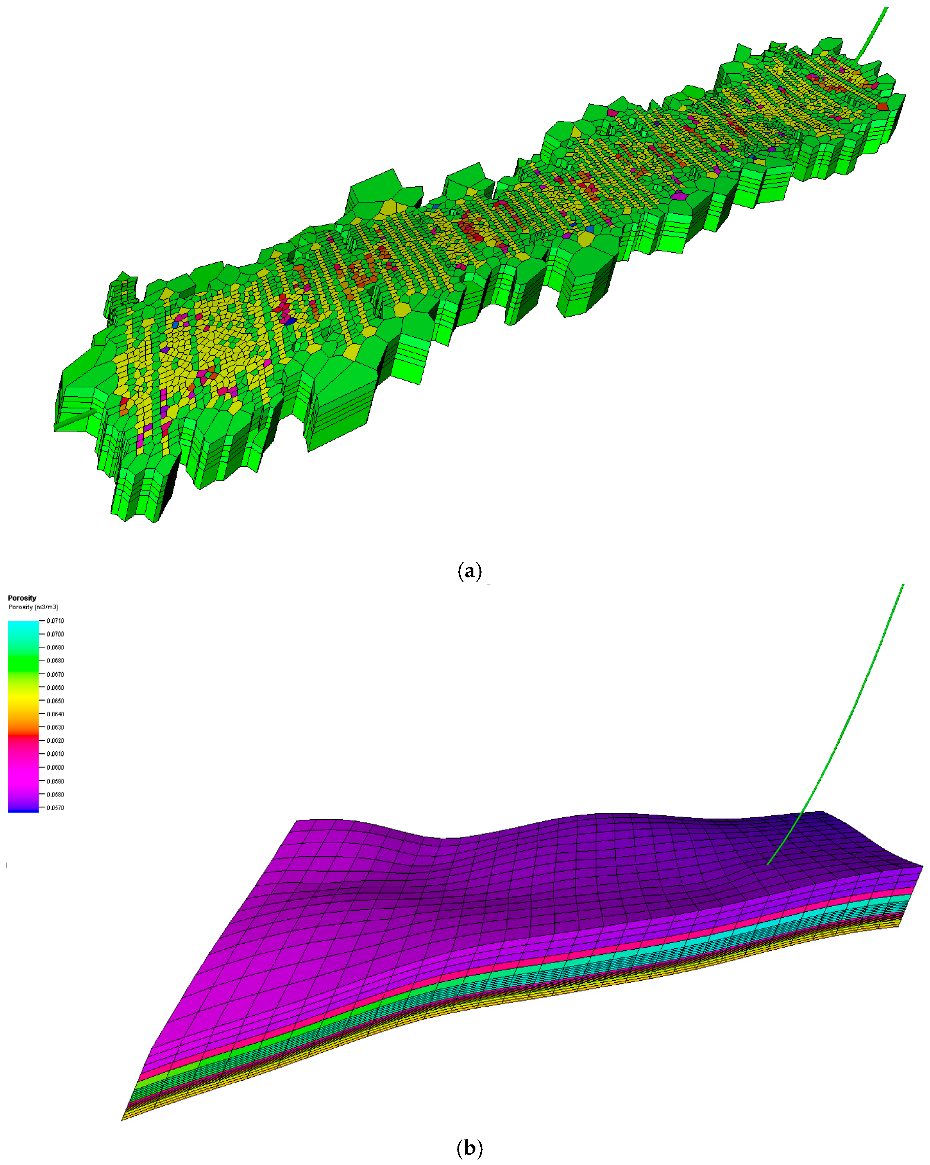
(4) The property model was established based on the structural model by discretizing the logging data, setting appropriate variograms, and using interpolation or stochastic simulation methods to predict the distribution of inter-well property parameters [31]. This approach was used to establish a three-dimensional property distribution model for the 13 wells in the South Sichuan areas (Figure 2).
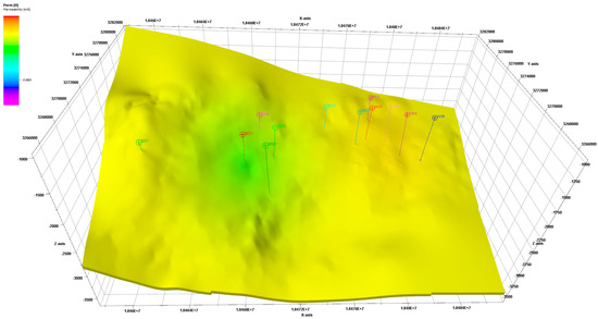
Figure 2.
Porosity property modeling.
4.2. Wellbore Modeling
4.2.1. UFM Governing Equations
The equilibrium model used to calculate the fracture height based on the pressure at different locations of the fracture is extended to a nonequilibrium model by considering the matching of the stress intensity factor to the fracture toughness of the corresponding layer, according to the method described by Kresse et al. [32]. The non-equilibrium height is increased by adding an apparent toughness proportional to the velocity at the top and bottom of the fracture, taking into account the pressure gradient generated by vertically oriented flow in the fracture tip region. The fracture width at any location z measured from the bottom of the fracture is given by Equation (1):
where is the fracture width as a function of depth at the current location, is the fluid pressure at the reference depth measured from the bottom of the fracture, and is the Young’s modulus.
In addition, the global volume balance condition by Equation (2) must be satisfied:
That is, the total amount of fluid pumped at time t is equal to the amount of fluid in the fracture network and the amount of fluid that leaked out of the fracture prior to time t. The boundary conditions are based on a net pressure of zero at the top of the fracture and a net pressure of zero at the top of the fracture. The boundary conditions are based on a net pressure of zero at the top of the fracture. The boundary condition requires that the flow rate, net pressure, and fracture width at the tops of all cracks be zero.
4.2.2. Wellbore Engineering Parameter Input and Calibration
In the study of wellbore flow, the setting of engineering parameters is crucial for accurately predicting flow characteristics and optimizing gas well production efficiency [33,34]. Therefore, based on the fracturing design, parameters for segmentation and cluster placement are established, and the perforation intervals of the target wells are clearly defined. Additionally, data related to the fracturing fluid properties, proppant properties, and completion tubing configurations are input into the model. Table 2 lists the key components of the input.
Table 2.
Key parameters of wellbore engineering.
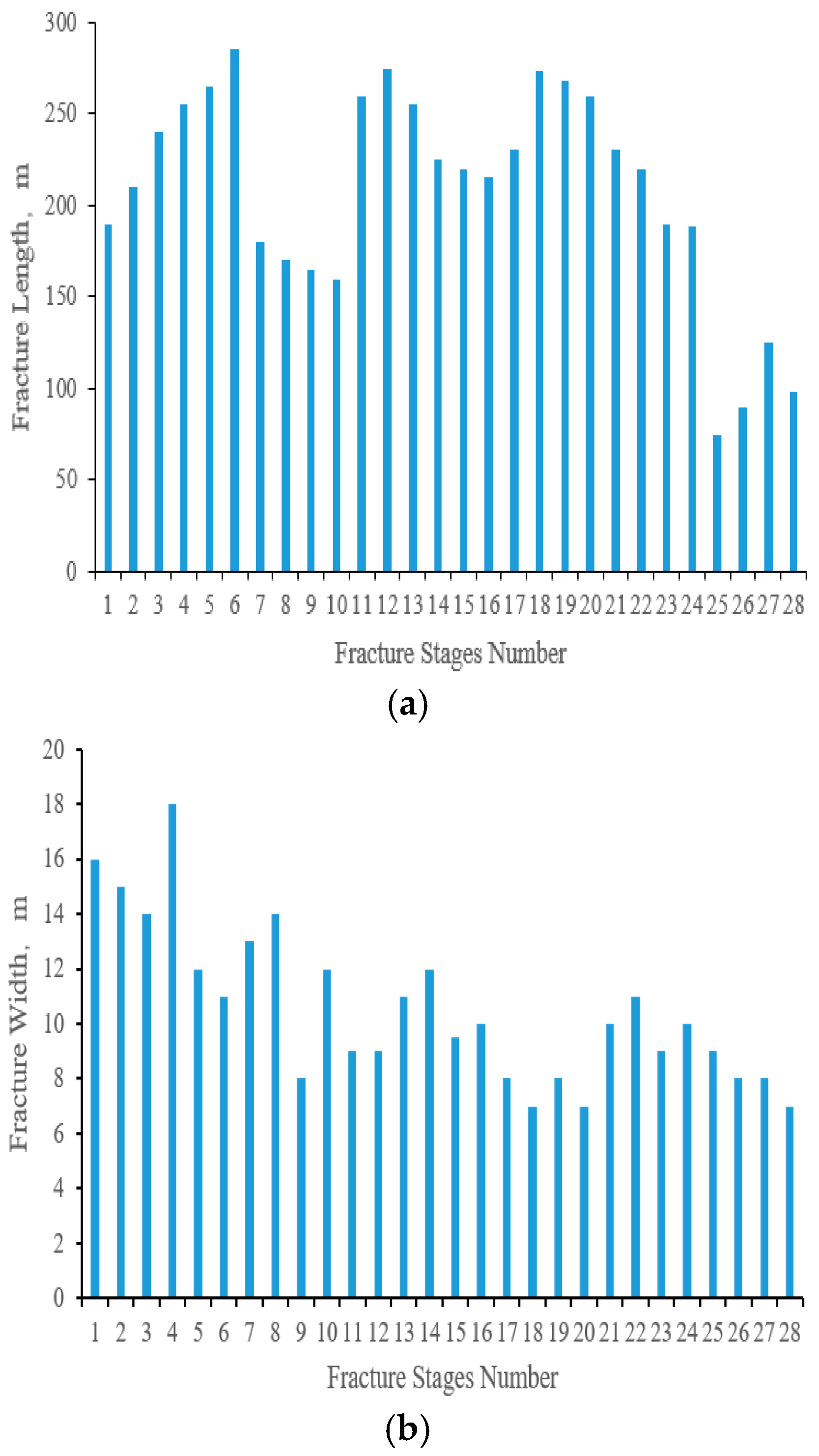
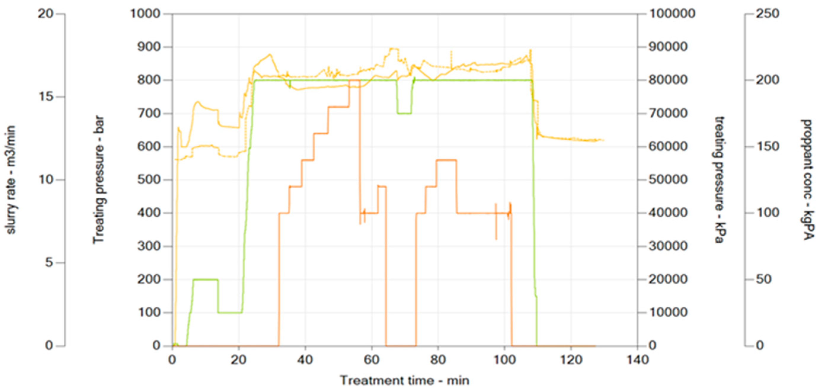
Using the pumping schedule from the fracturing design, appropriate fracturing fluids and proppants are selected to conduct simulations of fracture network propagation. The simulation accounts for inter-segment and inter-cluster stress interference and adjusts fracture height penetration based on actual in situ stress conditions. The UFM unstructured fracture propagation model is employed to simulate hydraulic fracture propagation during segmented and clustered fracturing (Figure 3). Following the sequence of fracturing operations, the model considers inter-well, inter-segment, and inter-cluster stress shadows to calculate the fracture propagation for each segment of the wells. The fracture length ranges from 70 to 290 m, with an average length of 210 m, while the fracture width ranges from 7 to 18 mm, with an average width of approximately 10.53 mm (Figure 4). The average fracture conductivity is 49.12 mD·m. By calibrating the model with the actual pumping schedule and comparing the simulated pressures with the actual fracturing pressures, most segments show good agreement (Figure 5). Through the input and correction of these wellbore engineering parameters, the wellbore model is refined and perfected.
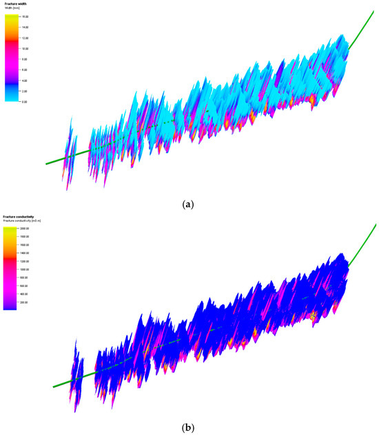
Figure 3.
Hydraulic fracturing expansion simulation scenario. (a) Distribution of fracture width. (b) Distribution of fracture conductivity.
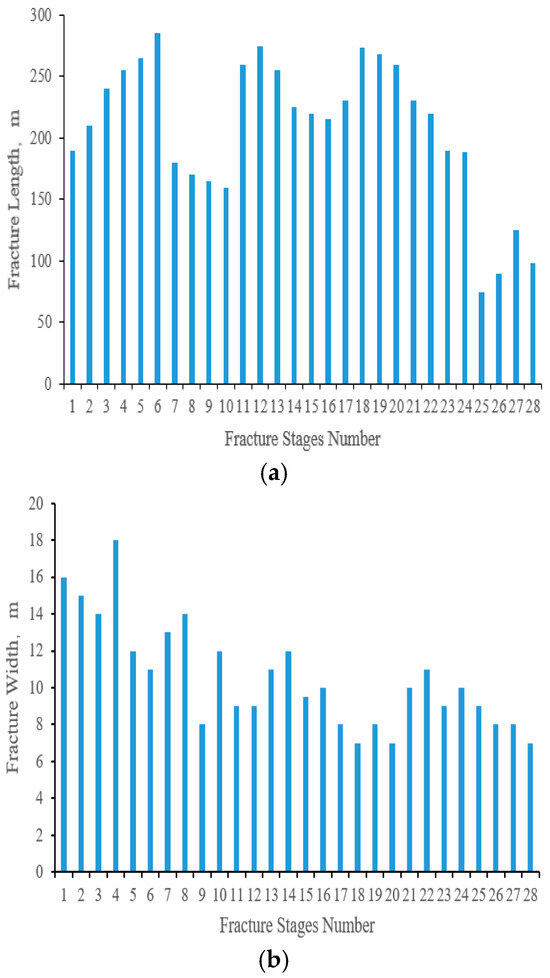
Figure 4.
Hydraulic fracturing expansion simulation results. (a) Distribution map of fracture length; (b) distribution map of fracture width.
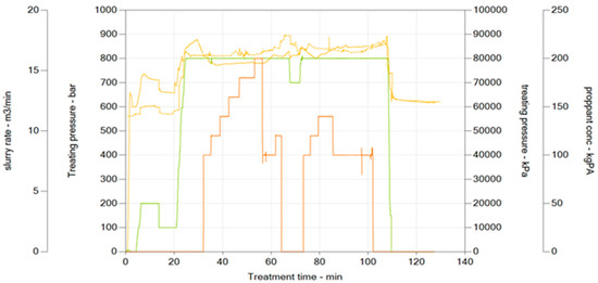
Figure 5.
Fracturing construction curve fitting.
4.3. Establishment of Gas Reservoir Models
Using the Petrel RE module, the reservoir near the target well was refined with enhanced gridding, coupled with an engineered fracture network to generate an unstructured grid and assign reservoir properties. Detailed property settings for each well were set using the software, and the development zones for each well were precisely delineated based on geological characteristics and reservoir properties.
Local grid refinement around the fractures was performed to achieve a detailed description of the reservoir near the fractures and more accurate simulation results, thereby providing a scientific basis for the efficient development of gas wells. A quadrilateral unstructured grid was employed, and the unstructured grid was divided according to the geological property model and fracture propagation simulation results (Figure 6). A numerical simulation grid model was established. To ensure the efficiency of numerical simulation, the fractures were equivalent, with an equivalent fracture grid size of 1 m.

Figure 6.
Grid partitioning. (a) Fracture propagation; (b) Geological property mode.
Different reservoir types correspond to distinct porosity and permeability characteristics, as well as relative permeability relationships. Moreover, there is a significant difference in relative permeability between the fractured and unfractured zones. To address this, different relative permeability curves are embedded into the model to differentiate between the fractured and unfractured zones. For the unfractured zone, a matrix relative permeability curve is assigned. The fluid in the fracture is dominated by fast flow with weak capillary forces, and Equation (3) is used as the model for embedding the relative permeability curves [35]:
where is the fracture residual gas saturation and is the fracture gas power law index.
Fluid in the matrix is dominated by slow osmosis, capillary forces dominate, and flow nonlinearity is strong [36]:
where is the matrix water saturation, is the matrix gas saturation, is the matrix bound water saturation, is the matrix residual gas saturation, and and are water and gas indices, respectively.
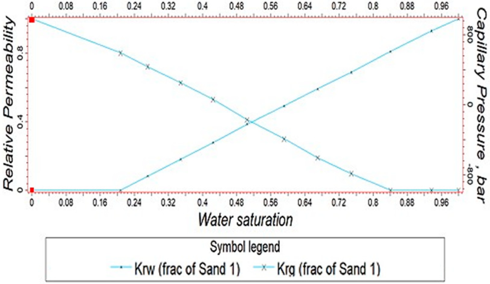
Since matrix relative permeability is difficult to obtain experimentally, it is typically initially assigned arbitrarily in numerical simulations and then adjusted through historical matching. The fracture relative permeability curve assigned to the fractured zone is shown in Figure 7.
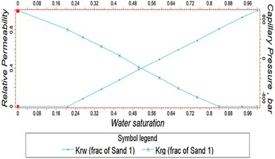
Figure 7.
Fracture − phase infiltration curves.
Due to the different sensitivities of the fracture and matrix to stress changes, a fracture is an open or semi-open structure that tends to deform when subjected to effective stresses, leading to a decrease in permeability. The control model of Equation (5) is used [37]:
where is the fracture permeability, is the initial fracture permeability, is the fracture stress sensitivity factor, is the original formation pressure, and is the formation pressure.
The pore structure of the matrix is stable, and the permeability varies less with stress, so the control model of Equation (6) is used [38]:
where is the matrix permeability, is the initial matrix permeability, and is the matrix stress sensitivity factor.
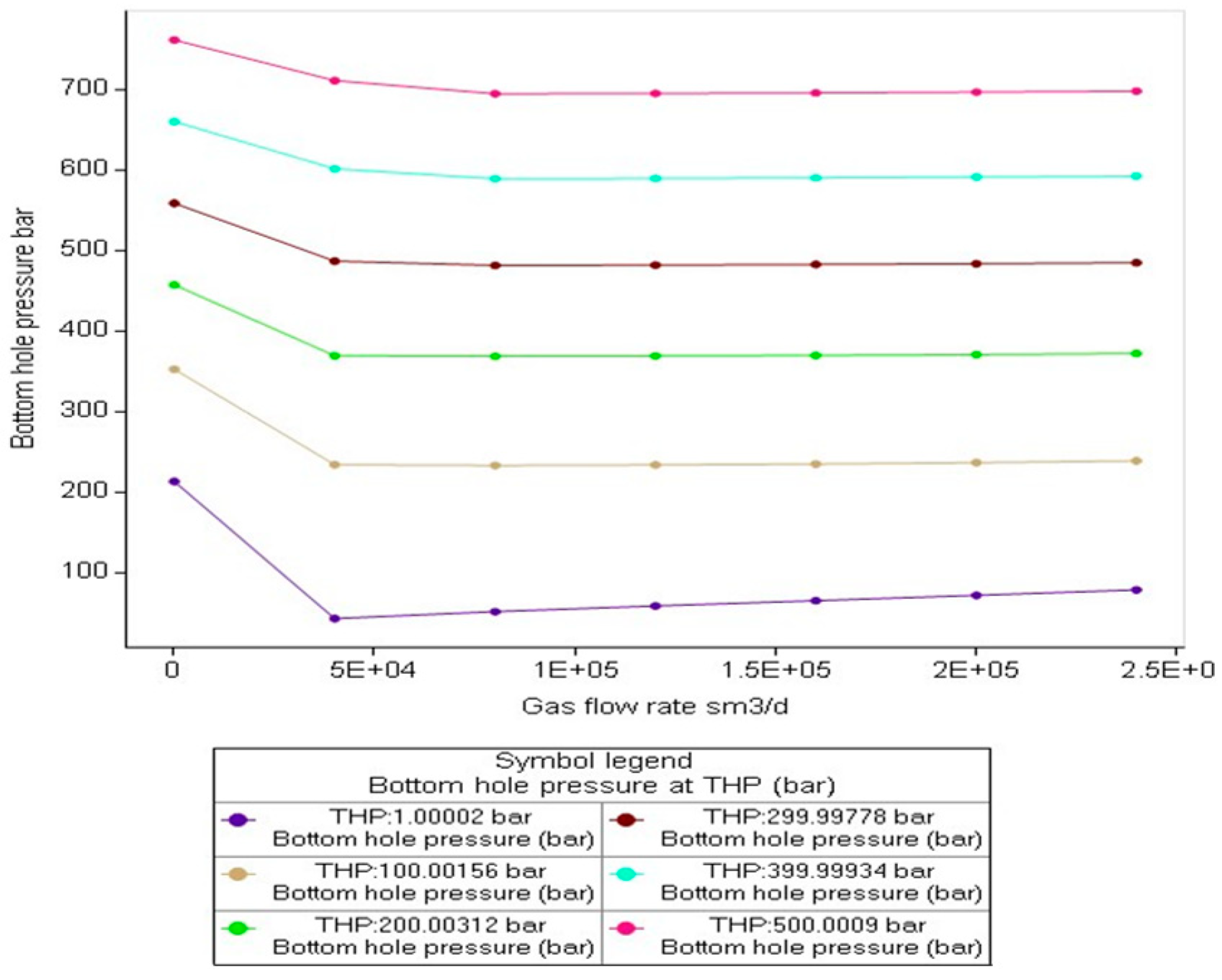
Therefore, different relative permeability and stress sensitivity curves are used for the fracture and matrix zones. To simulate the pressure variation from the wellhead to the bottom of the well and achieve historical matching of wellhead pressure, water production, and gas production, a wellbore flow VFP (vertical flow performance) model is established. The VFP model is fitted based on the relationship between the test pressure and gas and water production (Figure 8).
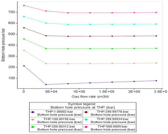
Figure 8.
Wellbore flow VFP model.
Through the grid division, local refinement, relative permeability curves, stress sensitivity, and the established VFP model, a complete gas reservoir model is constructed.
4.4. Validation of the Integrated Wellbore–Gas Reservoir Coupling Model
The corrected wellbore model is coupled with the established reservoir model. Subsequently, the Intersect unstructured grid reservoir simulation module is utilized to perform production history matching for individual wells on the platform. Historical gas production is used to fit the wellhead pressure and water production, with primary adjustments made to fracture and matrix permeability, water saturation, relative permeability curves, and stress sensitivity curves. The specific operation of historical matching is to prioritize the adjustment of fracture permeability, matrix permeability and water saturation to match the early production and pressure data. Due to the high sensitivity of the fracture permeability and water saturation parameters, the fracture permeability is adjusted in the range of ±50% without detracting from the reasonableness, and water saturation is adjusted in the range of ±10% by combining with the logging interpretation data; due to the slow flow of the matrix, the matrix permeability has lower sensitivity and is adjusted by ±20%. This is followed by the calibration of the stress sensitivity curve, fitting the decreasing trend of capacity in the middle and late stages by adjusting the sensitivity coefficients of the fracture and matrix, and finally fine-tuning the relative permeability curve to optimize the dynamic change in water content.
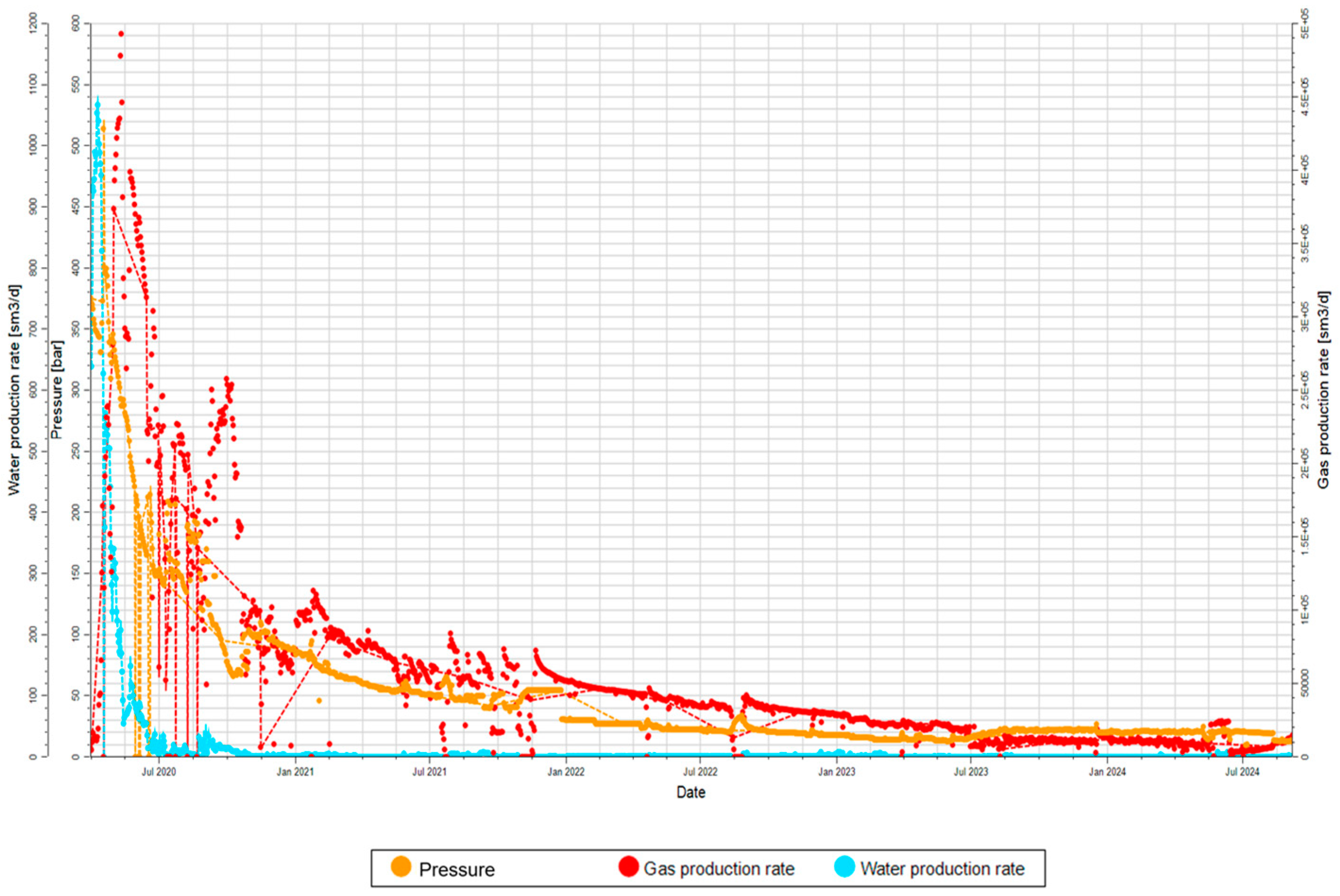
The geological model is employed to conduct production history matching for the 13 selected target wells (Figure 9 shows the fitting results for Well W01 in the south Sichuan block). The simulated trends in production and pressure align well with the actual production data of the wells. This validation confirms that the established integrated wellbore–gas reservoir coupling model is consistent with the actual conditions of the study block. It lays the groundwork for the subsequent analysis of the optimal pressurization timing and parameter optimization for compressors.
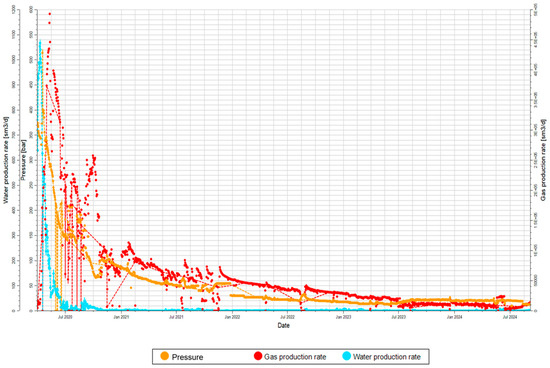
Figure 9.
Single-well fitting based on an established integration model.
5. Prediction of Pressurization Effects Based on an Integrated Model
Based on the integrated wellbore–gas reservoir coupling model established in this study, a simulation of the pressurization effects was conducted for the 13 target wells in the south Sichuan block (Table 3). A daily gas production rate of 4000 m3 was selected as the threshold for initiating pressurization. The wells were categorized into four classes (Classes I, II, III, and IV) according to the production increase after pressurization, with the boundaries for the four pressurization effects set at 20%, 10%, and 5%, respectively.
Table 3.
Comparison of production enhancement effects before and after pressurization.
Based on the classification criteria for the production increase, the following results were obtained:
(1) Class I Wells: Wells with a production increase exceeding 20%, including wells W02, W03, W04, and W07. These wells show significant production increases and make a substantial contribution to the overall field production.
(2) Class II Wells: Wells with a production increase between 10% and 20%, including wells S01 and S03. These wells exhibit noticeable production increases but have the potential for further improvement.
(3) Class III Wells: Wells with a production increase between 5% and 10%, including wells S02, S04, W06, and W09. These wells show moderate production increases and may require adjustments to their production enhancement strategies.
(4) Class IV Wells: Wells with a production increase below 5%, including wells W01, W05, and W08. These wells have relatively low production increases and may require further technical optimization.
6. Prediction of Pressurization Timing for Shale Gas Wells
6.1. Steps for Predicting Pressurization Timing in Shale Gas Wells
In the middle and late stages of shale gas well production, the rapid decline in bottom hole pressure often results in wellhead pressure falling below the gathering pipeline network pressure. This pressure deficiency can prevent the normal transportation of shale gas, thereby affecting the normal production of shale gas wells. To address this issue, the pressurization of shale gas wells is required.
Currently, most on-site operations divide shale gas blocks into different development zones for “rolling” development based on actual conditions. Under this “rolling” development model, the wellhead pressure and the gathering pipeline network pressure are constantly changing, making it difficult to determine the timing for pressurization. Therefore, it is necessary to integrate geological and reservoir engineering through joint analysis, adopting an innovative integrated wellbore–gas reservoir coupling model to determine the pressurization timing for shale gas wells.
The specific steps for predicting the pressurization timing of shale gas wells are as follows:
(1) Using an integrated geological and gas reservoir engineering approach, we combine a three-dimensional geological model, a mechanical model, and hydraulic fracture propagation simulation to establish an integrated wellbore–gas reservoir coupling model. This model is then verified by comparing it with actual production data to ensure its accuracy.
(2) Based on the existing decline patterns of gas production and wellhead pressure for shale gas wells, the integrated wellbore–gas reservoir coupling model is used to predict the changes in gas production at each future time point, thereby generating the estimated ultimate recovery (EUR) curve.
(3) By adjusting the efficiency of the compressor, the wellhead pressure can be effectively controlled. This enhances the instantaneous production flow rate of the shale gas well and optimizes its liquid-carrying capacity, ensuring effective shale gas extraction. To simulate and identify the optimal pressurization timing, different wellhead pressures are selected within the integrated wellbore–reservoir model to generate multiple EUR curves. By comparing the cumulative gas production values at the endpoints of these EUR curves, the best pressurization timing can be determined. The higher the cumulative production value, the better the corresponding pressurization timing.
6.2. Prediction of Pressurization Timing for Shale Gas Wells in the South Sichuan Block
Considering the actual conditions of shale gas wells in the South Sichuan Block, when the wellhead pressure drops below 4 MPa, it becomes difficult for the wells to continue producing gas.
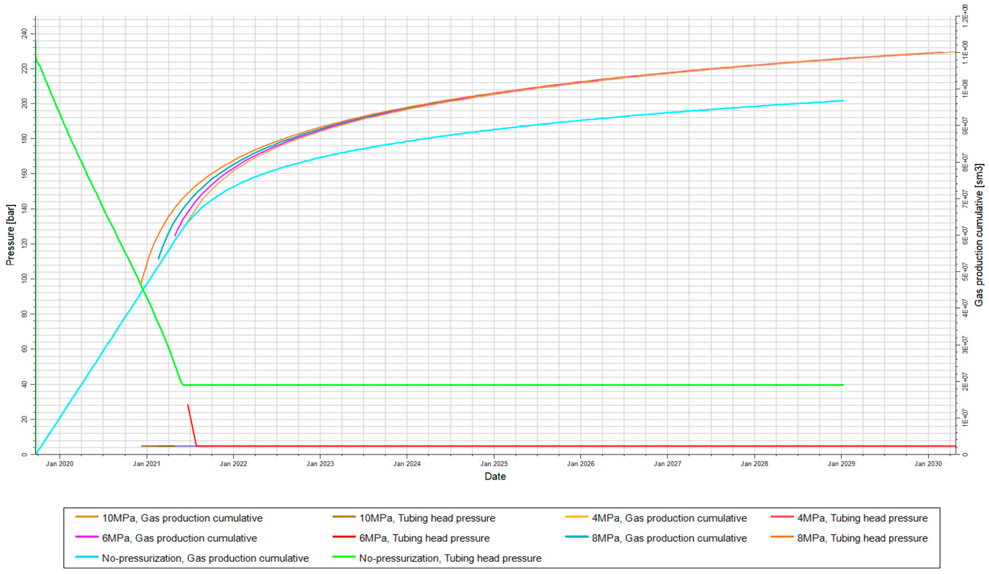
Additionally, taking economic factors into account, to prevent well losses, production must cease when the daily gas production of a shale gas well decreases to 3800 m3/d. Therefore, based on the integrated wellbore–gas reservoir coupling model established in this study, taking Well W01 in the South Sichuan Block as an example, four methods are adopted to optimize the timing of pressurization under the condition of ensuring that the wellhead pressure is below 4 MPa and the daily gas production remains above 3800 m3/d. These methods include initiating pressurization when the wellhead pressure drops to 10 MPa, 8 MPa, 6 MPa, and 4 MPa, respectively. Numerical simulations are conducted based on the established strategies, with the results shown in Figure 10 and Table 4.
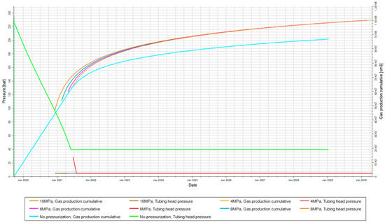
Figure 10.
Cumulative gas production vs. wellhead pressure graph.
Table 4.
Simulated EUR results for different pressurization timings.
When no pressurization is applied, it must be ensured that the wellhead pressure does not fall below the minimum allowable pressure of the gathering system. Considering the pipeline network pressure, the shale gas well must continue production at a wellhead pressure of 4 MPa. When the daily gas production decreases to below 3800 m3/d, the well is shut in. The EUR curve endpoint value at this point is 0.9694 billion cubic meters. According to on-site requirements, all wells in the block use the same model of pressurizer, which can reduce the bottom hole pressure of the shale gas well to 0.5 MPa. During normal production, when the bottom hole pressure drops to 10 MPa, the pressurizer is activated to reduce the bottom hole pressure to 0.5 MPa. The EUR curve shows a significant increase in production at this point. When maintaining production at a bottom hole pressure of 0.5 MPa until the daily gas production is insufficient to maintain economic viability (below 3800 m3/d), the well is shut in. The EUR curve endpoint value at this point is 1.1011 billion cubic meters. Compared to conditions of no pressurization, applying the pressurizer at a bottom hole pressure of 10 MPa increases the EUR by 0.1316 billion cubic meters, a growth of 13.58%. When the pressurizer is applied at a bottom hole pressure of 8 MPa, the EUR can be increased to 1.1020 billion cubic meters. Compared to no pressurization, the EUR increases by 0.1326 billion cubic meters, with a production increase of 13.68%. Applying the pressurizer when the bottom hole pressure drops below 6 MPa results in an EUR endpoint value of 1.1025 billion cubic meters. Compared to no pressurization, the EUR increases by 0.1330 billion cubic meters, a rise of 13.72%. When the pressurizer is applied at a bottom hole pressure of 4 MPa, the EUR reaches 1.1083 billion cubic meters. Compared to no pressurization, the EUR increases by 0.1388 billion cubic meters, with a production increase of 14.32%.
Therefore, as the pressurization timing is delayed from 10 MPa to 4 MPa, the cumulative gas production growth rate increases from 13.58% to 14.32%, and the EUR increment rises from 13.16 million cubic meters to 13.88 million cubic meters. It is evident that applying the pressurizer when the wellhead pressure drops to 4 MPa yields the best production enhancement effect.
7. Optimization of Pressurization Parameters for Shale Gas Wells
7.1. Selection of Pressurization Parameters for Shale Gas Wells
In the development of shale gas wells, the selection of pressurization parameters is crucial for enhancing the production efficiency and ultimate recovery rates. Typically, the location and pressure of the compressor are chosen as the optimization parameters. However, considering only the compressor location and pressure, while ignoring the impact of fluid flow in the reservoir, can compromise the accuracy of the optimized results.
Therefore, by fully considering the dynamic changes in wellhead pressure and gas production, this study proposes an innovative method of changing the pressurization regime by setting different pressurization rates, based on determining the optimal timing for pressurization. This method integrates both wellbore flow and reservoir seepage, resulting in more accurate optimized pressurization parameters that hold significant reference value for field applications.
7.2. Steps for Optimizing Pressurization Parameters of Shale Gas Wells
Based on determining the optimal pressurization timing, the pressurization regime is optimized by adjusting the pressurization rate of the compressor. The specific parameter optimization steps are as follows:
(1) First, it is necessary to obtain the power of the pressurizer used in the shale gas well and determine its maximum pressurization range. After obtaining the compressor power data, the maximum pressurization range is determined by combining the actual production data of the shale gas well (such as the wellhead pressure, cumulative gas production, etc.) and analyzing the performance of the pressurizer under different operating conditions (the stability and efficiency of the pressurizer at different wellhead pressures).
(2) On the basis of determining the optimal pressurization timing, the pressurization rate of the compressor is changed until it reaches the maximum pressurization range of the compressor. Four pressurization regimes are used for production dynamic predictions: average stepwise pressurization, accelerated stepwise pressurization, decelerated stepwise pressurization, and one-time pressurization. Average stepwise pressurization refers to the production of the compressor at the working pressure at the optimal pressurization timing. When production does not meet the economic limit acceptable to the well area, the efficiency of the pressurizer is increased at an average rate. Each adjustment increases the daily gas production. When the daily gas production is insufficient to meet the requirements of the well area, the pressurization efficiency is adjusted on average until the maximum pressurization range is reached. Accelerated stepwise pressurization involves gradually increasing the pressurization efficiency of the compressor from slow to fast. After each adjustment, when the daily production again reaches the minimum acceptable level of the well area, the pressurization efficiency is changed. Decelerated stepwise pressurization involves adjusting the pressurization efficiency of the compressor from fast to slow, and, similarly, the pressurization efficiency is changed when the daily production limit is reached. One-time pressurization involves directly adjusting the power of the pressurizer to the maximum pressurization efficiency at the optimal pressurization timing. When daily production is insufficient to meet the requirements of the well area, production is stopped after reaching the minimum daily production limit.
(3) On the integrated wellbore–gas reservoir coupling model with the determined optimal pressurization timing, five different pressurization regimes (no pressurization, average stepwise pressurization, accelerated stepwise pressurization, decelerated stepwise pressurization, and one-time pressurization) are set and input into the model to obtain five different EUR curves. By comparing these five different EUR curves, the optimal pressurization regime is determined.
7.3. Parameter Optimization for the South Sichuan Shale Gas Wells
To optimize the pressurization parameters for shale gas wells, taking well W01 in the South Sichuan Block as an example, this study adjusted the pressurization regime based on the determined optimal pressurization timing (when the wellhead pressure reaches 4 MPa) and the integrated wellbore–reservoir model. The compressor can reduce the wellhead pressure from 4 MPa to a minimum of 0.5 MPa. Four different pressurization regimes were tested through production dynamic prediction by changing the pressurization rate. These regimes include average stepwise pressurization, accelerated stepwise pressurization, decelerated stepwise pressurization, and one-time pressurization.
Considering that the minimum acceptable daily gas production in the South Sichuan Block is 3800 m3, the average stepwise pressurization regime involves starting the compressor when the wellhead pressure reaches 4 MPa during normal production to reduce the pressure to 3 MPa. Production continues until the daily gas production falls below 3800 m3, at which point the wellhead pressure is further reduced to 2 MPa. This process is repeated, with the pressure being reduced to 1 MPa and finally to 0.5 MPa, until the daily gas production no longer meets the requirements, at which point the well is shut in.
Accelerated stepwise pressurization involves starting the compressor when the wellhead pressure drops to 4 MPa. The compressor efficiency is then adjusted in sequence at wellhead pressures of 3.5 MPa, 3 MPa, 2.5 MPa, 1 MPa, and 0.5 MPa whenever the daily gas production falls below 3800 m3. Production continues until the daily gas production no longer meets the minimum requirement at a wellhead pressure of 0.5 MPa, at which point the well is shut in.
Decelerated stepwise pressurization is similar to the previous two regimes but changes the rate of pressurization, starting with a rapid increase followed by a gradual increase. The sequence of wellhead pressure adjustments is 2.5 MPa, 1.5 MPa, 1 MPa, and 0.5 MPa.
One-time pressurization involves starting the compressor when the wellhead pressure drops to 4 MPa and directly reducing the wellhead pressure to 0.5 MPa.
To compare the results after parameter optimization, the outcomes need to be contrasted with those of wells that have not undergone pressurization.
(1) Average stepwise pressurization (4 MPa→3 MPa→2 MPa→1 MPa→0.5 MPa)
(2) Accelerated stepwise pressurization (4 MPa→3.5 MPa→3 MPa→2.5 MPa→1 MPa→0.5 MPa)
(3) Decelerated stepwise pressurization (4 MPa→2.5 MPa→1.5 MPa→1 MPa→0.5 MPa)
(4) One-time pressurization (4 MPa→0.5 MPa)
(5) No pressurization (Normal Production)
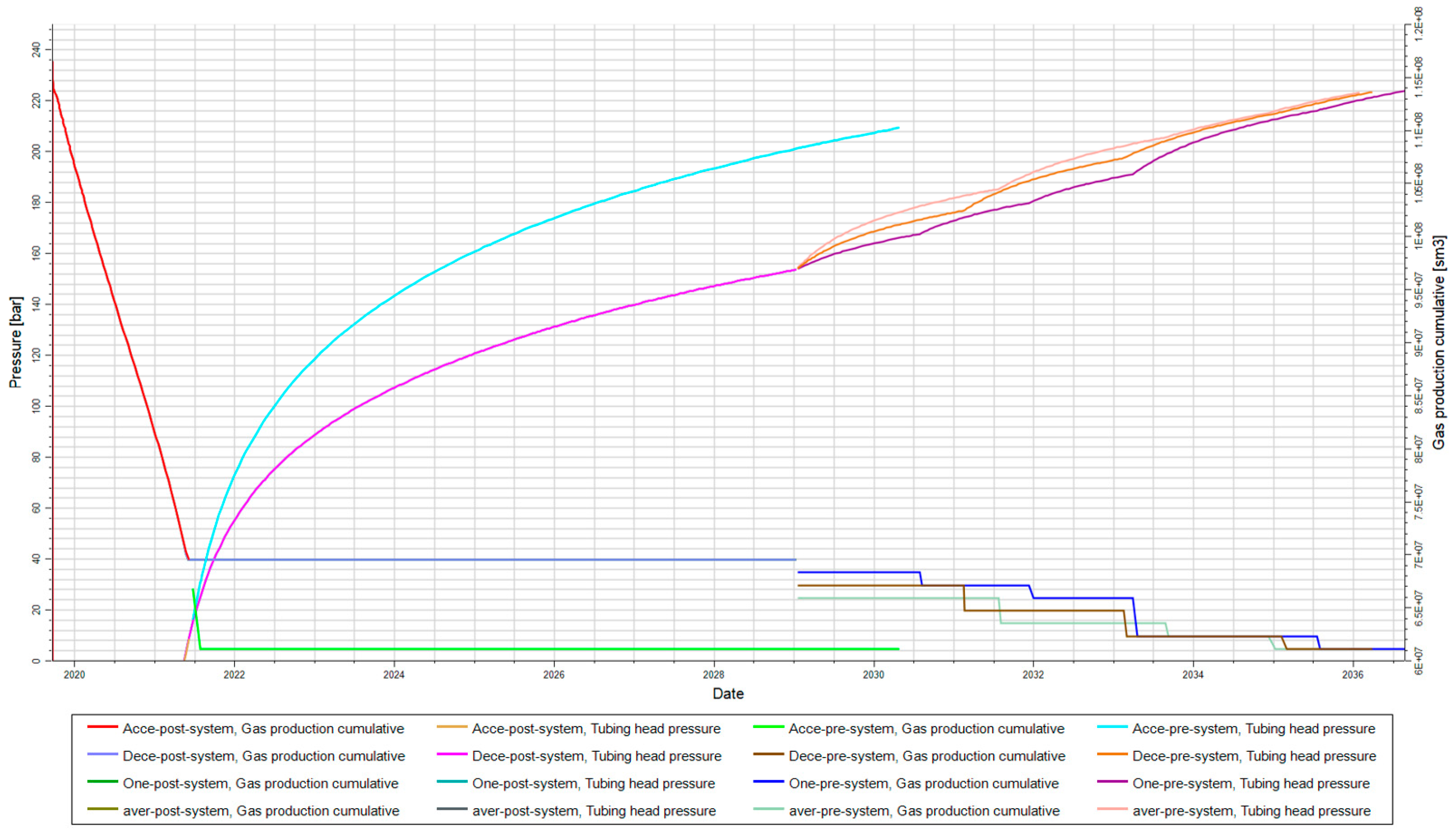
The pressurization regimes were implemented as strategies and input into the model, resulting in five distinct EUR curves (Figure 11). The EUR endpoint value for the well without pressurization is 0.9694 billion cubic meters of gas. For average stepwise pressurization, the EUR endpoint value is 1.1336 billion cubic meters of gas, which is an increase of 0.1642 billion cubic meters compared to no pressurization, representing a growth of 16.93%. The EUR curve endpoint for accelerated stepwise pressurization corresponds to 1.1381 billion cubic meters of gas, with an increase of 0.1687 billion cubic meters compared to no pressurization, resulting in a 17.40% increase after the measurement. For decelerated stepwise pressurization, the EUR reaches 1.1339 billion cubic meters of gas, which is an increase of 0.1645 billion cubic meters compared to before the measurement, with a 16.97% increase in cumulative gas production after the measurement. For one-time pressurization, the EUR curve endpoint value is 1.1025 billion cubic meters of gas, which is an increase of 0.1338 billion cubic meters compared to no pressurization, with a 14.32% increase in cumulative gas production.
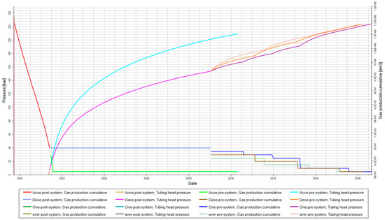
Figure 11.
Cumulative gas production vs. wellhead pressure graph.
By comparing the simulated EUR results under the five different pressurization regimes, accelerated stepwise pressurization achieves a higher EUR. Compared to one-time pressurization, the EUR is increased by 3.49 million cubic meters, and the cumulative gas growth rate rises from 14.32% to 17.40%, showing a significant enhancement in production (Table 5).
Table 5.
Simulated EUR results for different pressurization regimes.
8. Conclusions
(1) An integrated continuous flow model linking the reservoir, fractures, and wellbore after hydraulic fracturing was established by combining a three-dimensional geological model, a mechanical model, fracture propagation simulations, and reservoir numerical simulations. This integrated wellbore–gas reservoir coupling model enables comprehensive production dynamic analysis and prediction. The model couples the wellbore and reservoir, providing a holistic representation of fluid flow during production.
(2) Based on the established integrated wellbore-gas reservoir coupling model, the optimal pressurization timing was selected for wells in the South Sichuan Block through dynamic analysis. Taking well W01 as an example, the best pressurization timing was determined to be when the wellhead pressure drops to 4 MPa, with the production increase rate reaching 14.32% after the measurement.
(3) Under the condition of determined pressurization timing, the pressurization parameters were optimized, and the pressurization regime was adjusted. The analysis showed that the optimal pressurization regime is accelerated stepwise pressurization, which increases the production increase rate to 17.40%, showing a significant enhancement in production.
9. Prospects
Although this study has achieved some results in the construction of an integrated wellbore–gas reservoir coupling model and the optimization of pressurization timing and parameters, it has some limitations. First, this study mainly analyzes a single gas well and does not fully consider the mutual interference effect when multiple wells are pressurized at the same time, whereas, in actual production, multiple wells are often operated at the same time, and their interference may have an impact on the pressurization effect. Second, the fracture geometries used in the study are based on simulation results, which may show some deviation from the actual values, and different fracture geometries may have different effects on the production dynamics of gas wells. In addition, this study mainly focuses on shale gas wells, and the optimization of pressurization strategies for other types of reservoirs, such as condensate reservoirs, has not yet been addressed. Future research can be further carried out in the following directions: first, an in-depth study of the influence of multi-well interference effects on the pressurization effect, and the establishment of a multi-well coupling model for comprehensive analysis; second, further optimization and verification of the accuracy of fracture geometries in conjunction with the actual field data, to explore their sensitivity to the optimization of pressurization timing and parameters; third, to extend the research method to other types of reservoirs, such as condensate reservoirs, to explore the optimization methods of pressurization strategies under different reservoir conditions, and to provide more comprehensive technical support for oil and gas field development.
Author Contributions
Conceptualization, Y.P.; Methodology, Z.L.; Validation, W.L.; Formal analysis, Y.Y.; Investigation, Q.Z.; Resources, J.Z.; Writing—original draft, F.H.; Writing—review & editing, Y.C.; Visualization, H.M. All authors have read and agreed to the published version of the manuscript.
Funding
This study was supported by the National Natural Science Foundation of China (No. 52204051, U23B20156, 52304046, 52174033), the Science and Technology Cooperation Project of the CNPC-SWPU Innovation Alliance (No. 2020CX030202).
Data Availability Statement
The data are unavailable due to privacy.
Conflicts of Interest
Author Yusong Chen, Feng He, Yadong Yang and Qike Zheng was employed by Shale Gas Exploration and Development Department, CNPC Chuanqing Drilling Engineering Company Limited. The remaining authors declare that the research was conducted in the absence of any commercial or financial relationships that could be construed as a potential conflict of interest.
References
- Fan, Y.; Chen, J.; Xiang, J.; Ye, C.; Han, G. Intermittent Optimization of Shale Gas Wells Based on Reservoir–Wellbore Coupling. Processes 2025, 13, 247. [Google Scholar] [CrossRef]
- Su, H.; Zhang, K.; Nie, H.; Guo, S.; Li, P.; Sun, C. High-Quality Reservoir Space Types and Controlling Factors of Deep Shale Gas Reservoirs in the Wufeng–Longmaxi Formation, Sichuan Basin. Energy Fuels 2025, 39, 1106–1125. [Google Scholar]
- Daryasafar, A.; Shahbazi, K.; Ghadiri, M.; Marjani, A. Simultaneous geological CO2 sequestration and gas production from shale gas reservoirs: Brief review on technology, feasibility, and numerical modeling. Energy Sources Part A Recovery Util. Environ. Eff. 2025, 47, 1472–1489. [Google Scholar]
- Ju, Y.W.; Hou, X.G.; Han, K.; Song, Y.; Xiao, L.; Huang, C.; Zhu, H.J.; Tao, L.R. Experimental deformation of shales at elevated temperature and pressure: Pore-crack system evolution and its effects on shale gas reservoirs. Pet. Sci. 2024, 21, 3754–3773. [Google Scholar]
- Xu, Y.; Liu, X.; Hu, Z.; Duan, X.; Chang, J. Bottom-hole pressure drawdown management of fractured horizontal wells in shale gas reservoirs using a semi-analytical model. Sci. Rep. 2022, 12, 22490. [Google Scholar]
- Rahimi-Agham, S.; Chau, V.T.; Lee, H.; Nguyen, H.; Li, W.; Karra, S.; Rougier, E.; Viswanathan, H.; Srinivasan, G.; Bazant, Z.P. Branching of Hydraulic Cracks in Gas or Oil Shale with Closed Natural Fractures: How to Master Permeability. Proc. Natl. Acad. Sci. USA 2019, 116, 1532–1537. [Google Scholar]
- Liu, S.; Wu, J.; Yang, X.; Xie, W.; Chang, C. Evaluation and Application of Flowback Effect in Deep Shale Gas Wells. Fluid Dyn. Mater. Process. 2024, 20, 2301–2321. [Google Scholar]
- Duan, X.; Xu, Y.; Xiong, W.; Hu, Z.; Gao, S.; Chang, J.; Ge, Y. Experimental and numerical study on gas production decline trend under ultralong-production-cycle from shale gas wells. Sci. Rep. 2023, 13, 10726. [Google Scholar]
- Shi, W.; Zhang, C.; Jiang, S.; Liao, Y.; Shi, Y.; Feng, A.; Young, S. Study on pressure-boosting stimulation technology in shale gas horizontal wells in the Fuling shale gas field. Energy 2022, 254, 124364. [Google Scholar]
- Ma, X.; Wang, H.; Zhao, Q.; Liu, Y.; Zhou, S. “Extreme utilization” development of deep shale gas in southern Sichuan Basin, SW China. Pet. Explor. Dev. 2022, 49, 1377–1385. [Google Scholar]
- Zhang, C.; Chen, S.; Zhu, S.; Yan, X.; Wang, H.; Wang, Y.; Li, J.-S.; Nie, R.-S. Modelling pressure dynamics of oil–gas two-phase flow in double-porosity media formation with permeability-stress sensitivity. Sci. Rep. 2024, 14, 24418. [Google Scholar]
- Wang, H.; Xia, L. Optimization of pressure drop model for shale gas wells in area X based on correlation coefficient method. In IOP Conference Series: Earth and Environmental Science; IOP Conference Series: Earth and Environmental Science; IOP Publishing: Bristol, UK, 2021; Volume 12056. [Google Scholar]
- Zhang, J.; Guo, B. Use of Pressure Transient Analysis Method to Evaluate the Effectiveness of Fluid-Soaking in Multi-Fractured Shale Gas Wells. Preprints 2024. [Google Scholar] [CrossRef]
- Zhu, Q.; Lin, B.; Yang, G.; Wang, L.; Chen, M. Intelligent production optimization method for a low pressure and low productivity shale gas well. Pet. Explor. Dev. 2022, 49, 886–894. [Google Scholar]
- Wang, Q.; Zhao, J.; Hu, Y.; Li, Y.; Wang, Y. Optimization method of refracturing timing for old shale gas wells. Pet. Explor. Dev. 2024, 51, 213–222. [Google Scholar]
- Chen, Z.; Nie, S.; Li, T.; Lai, T.; Huang, Q.; Zhang, K. Torsional vibration response characteristics and structural optimization of shale gas compressor shaft system. Proc. Inst. Mech. Eng. Part E J. Process Mech. Eng. 2022, 236, 1256–1266. [Google Scholar]
- Drouven, M.G.; Grossmann, I.E. Mixed-integer programming models for line pressure optimization in shale gas gathering systems. J. Pet. Sci. Eng. 2017, 157, 1021–1032. [Google Scholar] [CrossRef]
- Hong, B.; Li, X.; Cui, X.; Gao, J.; Li, Y.; Gong, J.; Liu, H. General Optimization Model of Modular Equipment Selection and Serialization for Shale Gas Field. Front. Energy Res. 2021, 9, 711974. [Google Scholar]
- Zhou, J.; Zhang, H.; Li, Z.; Liang, G. A MINLP model for combination pressurization optimization of shale gas gathering system. J. Pet. Explor. Prod. Technol. 2022, 12, 3059–3075. [Google Scholar]
- Wu, K.; Yang, J.; Lin, Y.; Zhou, P.; Luo, Y.; Wang, F.; Liu, S.; Zhou, J. A Multi-Period Model of Compressor Scheme Optimization for the Shale Gas Gathering and Transportation System. Processes 2023, 11, 3101. [Google Scholar] [CrossRef]
- Fu, X.; Khairullin, M.K.; Wei, J.; Shamsiev, M.N.; Abdullin, A.I.; Zhou, X.; Gadilshina, V.R.; Nasybullin, A.V.; Sultanov, S.K. Characterization of vertical well fluid inflow in fractured porous reservoirs with bottom-hole pressure below bubble point pressure. Heat Mass Transf. 2025, 61, 14. [Google Scholar]
- Chen, S.; Yu, Z.; Li, Y.; Wang, Z.; Si, M. Optimization of a Typical Gas Injection Pressurization Process in Underground Gas Storage. Sustainability 2024, 16, 8902. [Google Scholar] [CrossRef]
- Chen, D.; Huang, C.; Wei, M. Shale Gas Production Prediction Based on PCA-PSO-LSTM Combination Model. J. Circuits Syst. Comput. 2024, 33, 1. [Google Scholar] [CrossRef]
- Wei, X.; Huang, W.; Liu, L.; Wang, J.; Cui, Z.; Xue, L. Low-rank coalbed methane production capacity prediction method based on time-series deep learning. Energy 2024, 311, 133247. [Google Scholar] [CrossRef]
- Werneck, L.F.; Heringer, J.D.; de Souza, G.; Amaral Souto, H.P. Numerical simulation of non-isothermal flow in oil reservoirs using a coprocessor and the OpenMP. Comput. Appl. Math. 2023, 42, 365. [Google Scholar] [CrossRef]
- Peng, Y.; Luo, A.; Li, Y.; Wu, Y.; Xu, W.; Sepehrnoori, K. Fractional model for simulating Long-Term fracture conductivity decay of shale gas and its influences on the well production. Fuel 2023, 351, 129052. [Google Scholar] [CrossRef]
- Peng, Y.; Zhao, J.; Sepehrnoori, K.; Li, Z. Fractional model for simulating the viscoelastic behavior of artificial fracture in shale gas. Eng. Fract. Mech. 2020, 228, 106892. [Google Scholar] [CrossRef]
- Peng, Y.; Zhao, J.; Sepehrnoori, K.; Li, Z.; Xu, F. Study of delayed creep fracture initiation and propagation based on semi-analytical fractional model. Appl. Math. Model. 2019, 72, 700–715. [Google Scholar] [CrossRef]
- Zou, T.; Zuo, Y.; Meng, L.; Liu, Y.; Xing, X.; Feng, J. Application of geological modeling technology in secondary development of old and complex fault block oilfields. Oil Gas Geol. 2014, 35, 143–147. [Google Scholar]
- Caumon, G.; Collon-Drouaillet, P.L.; Le Carlier de Veslud, C.; Viseur, S.; Sausse, J. Surface-Based 3D Modeling of Geological Structures. Math. Geosci. 2009, 41, 927–945. [Google Scholar]
- Li, Z.; Peng, Y.; Peng, H.; Peng, J.; Li, Z. Simulation of borehole shrinkage in shale based on the triaxial fractional constitutive equation. Geomech. Geophys. Geo-Energy Geo-Resour. 2022, 8, 65. [Google Scholar] [CrossRef]
- Kresse, O.; Weng, X. Numerical Modeling of 3D Hydraulic Fractures Interaction in Complex Naturally Fractured Formations. Rock Mech. Rock Eng. 2018, 51, 3863–3881. [Google Scholar]
- Peng, Y.; Ye, J.; Li, Y.; Chen, Y.; Li, Z.; Zhang, D. Development and Performance Evaluation of Novel Self-Degradable Preformed Particulate Gels with High-Temperature and High-Salinity Resistance. SPE J. 2025, 30, 1105–1115. [Google Scholar]
- Zhijun, L.; Haiyin, W.; Hongfeng, W. Forecasting of Distribution of Tectonic Fracture by Principal Curvature Method Using Petrel Software. In Proceedings of the 2012 International Conference of Modern Computer Science and Applications, Wuhan, China, 8 September 2012; pp. 405–411. [Google Scholar]
- Lomeland, F.; Ebeltoft, E.; Thomas, W.H. A New Versatile Relative Permeability Correlation. In Proceedings of the International Symposium of the Society of Core Analysts, SCA2005-32, Toronto, ON, Canada, 21–25 August 2005. [Google Scholar]
- Gong, Y.; Sedghi, M.; Piri, M. Two-Phase Relative Permeability of Rough-Walled Fractures: A Dynamic Pore-Scale Modeling of the Effects of Aperture Geometry. Water Resour. Res. 2021, 57, e2021WR030104. [Google Scholar]
- Ghanbarian, B.; Liang, F.; Liu, H.-H. Modeling gas relative permeability in shales and tight porous rocks. Fuel 2020, 272, 117686. [Google Scholar]
- Li, M.; Bi, G.; Zhan, J.; Dou, L.; Xu, H. A Semianalytical Two-Phase Imbibition Model in Dual-Porosity and Dual-Permeability Reservoirs. Geofluids 2021, 2021, 5589936. [Google Scholar]


Disclaimer/Publisher’s Note: The statements, opinions and data contained in all publications are solely those of the individual author(s) and contributor(s) and not of MDPI and/or the editor(s). MDPI and/or the editor(s) disclaim responsibility for any injury to people or property resulting from any ideas, methods, instructions or products referred to in the content. |
© 2025 by the authors. Licensee MDPI, Basel, Switzerland. This article is an open access article distributed under the terms and conditions of the Creative Commons Attribution (CC BY) license (https://creativecommons.org/licenses/by/4.0/).