Anomaly Monitoring Model of Industrial Processes Based on Graph Similarity and Applications

Abstract

Aiming at the strong spatio-temporal coupling relationship between data in the actual industrial production process, which leads to the problem of insufficient reliability and poor timeliness of traditional process anomaly monitoring methods, a time series anomaly monitoring model based on the graph similarity network with multi-scale features is proposed, which can react to the anomalies in the process in a timely and effective manner to guarantee production safety. First, a graph-building method for spatio-temporally coupled time-series data using multidimensional time-varying feature map embedding is designed to capture the dependence of the data on time, while the topology of the graph is utilized to learn the spatial coupling of the data; second, a graph similarity-based anomaly monitoring strategy is innovatively proposed to measure the anomalies of the process using the difference degree index between the standard normal process data and the monitoring data. Finally, the proposed method is validated using the standard normal operating condition data of the Tennessee-Eastman (TE) process as well as the standard fault data. The experimental results show that the proposed model can identify anomalies more quickly and accurately than other typical methods, which significantly improves the reliability and timeliness of industrial process anomaly monitoring.

1. Introduction

With the continuous expansion of the production scale of industrial processes, the abnormal monitoring of industrial process operation status is of great significance in improving product quality and ensuring production safety [1,2]. The distributed control system (DCS) is widely used in the field of industrial control, so the complex industrial process of multi-dimensional spatial and temporal coupling of real-time acquisition and processing of time series data has become a reality. The in-depth analysis of process data can accurately reflect the operating status of industrial processes, providing unprecedented opportunities for process anomaly monitoring and diagnosis.

Data-based process monitoring methods have become one of the hot directions in the research field of industrial operation conditions, but the existing anomaly monitoring methods face many challenges [3,4,5,6]. First, multivariate statistics-based process anomaly monitoring methods usually monitor whether the statistics exceed the control limits to determine whether the process is anomalous or not. For example, principal component analysis (PCA) detects anomalies by reducing dimensionality and reconstruction errors and is suitable for high-dimensional linear data [7,8]; independent component analysis (ICA) detects anomalies by separating independent components, which is suitable for complex, non-Gaussian signals [9]; partial least squares (PLS) detects process anomalies and assists in troubleshooting by extracting latent variables and monitoring residuals or statistics [10]. The above methods are based on linear assumptions that make it difficult to capture nonlinear relationships, while ignoring the dependence on time and space leading to insufficient modeling of temporal features, which affects their effectiveness in complex systems. Second, deep learning-based process anomaly monitoring methods such as convolutional neural networks predict target values by modeling the process through a black box model, and anomaly monitoring is performed by comparing the predicted values with the observed values. While CNNs are able to capture local patterns and spatial dependencies, their inherent local feel-good field design makes it difficult to model global spatio-temporal dependencies, especially in industrial processes where there are long-range dependencies between variables, and CNNs are often limited in their performance [11,12]. Long short-term memory (LSTM) networks are suitable for time-series data and are capable of capturing temporal dependencies. However, its weak ability to model spatial features and the significant increase in computational complexity and training time when dealing with high-dimensional multivariate data limit its application in real industrial scenarios [13,14].

Image-based anomaly monitoring techniques for robust processes also play an irreplaceable role. References [15,16] use a deep learning approach to visual modeling to address the limitations of traditional inspection methods on non-planar objects and the challenges of defect detection in the presence of data scarcity. Graph-based methods have significant advantages and complementarities over traditional image-based defect detection methods. Image-based methods excel in processing visual information, especially in surface defect detection (e.g., scratches and cracks), and are able to effectively capture localized features of the image. Graph-based methods are better able to capture complex nonlinear relationships and global dependency structures in multidimensional spatio-temporal data by representing the data as graph structures. The two complement each other and provide new research ideas and application prospects for industrial process anomaly monitoring. The complexity of multidimensional spatio-temporal data is not only reflected in the high dimensionality and nonlinearity, but also in the dynamic coupling relationship between variables and spatio-temporal heterogeneity, which puts forward higher requirements on the generalization ability and robustness of the model.

Industrial processes have their unique operational characteristics: first, production processes often need to be maintained in steady state or show periodic changes for a long time to ensure the stability of product quality; second, due to the high reliability of modern industrial systems, the probability of failures occurring is extremely low, leading to a scarcity of anomaly samples, which brings significant difficulties to data-driven anomaly detection methods. However, this specificity also provides new research ideas for anomaly monitoring. The properties of steady-state processes imply that when an abnormality occurs, there is a significant difference between the abnormal working condition and the standard normal working condition. Therefore, accurate identification of abnormal states in a production process can be achieved by effectively capturing this dissimilarity through mathematical methods [17,18]. Further, the measure of dissimilarity between working conditions can be transformed into a similarity calculation problem, which provides a quantifiable evaluation framework for anomaly detection. Although traditional similarity calculation methods (e.g., Euclidean distance, cosine similarity, dynamic time regularization) perform well in specific scenarios, their limitations gradually emerge when facing high-dimensional, nonlinear, and spatio-temporally heterogeneous industrial data [19,20,21,22,23,24]. It is often difficult for these methods to comprehensively capture the complex relationships among data, leading to their lack of reliability and timeliness in industrial process anomaly monitoring. Therefore, how to design more adaptable similarity measures by combining the specificity of industrial processes is still an important direction of current research.

The graph-based similarity computation method opens up a brand new research direction for similarity computation and demonstrates a wide range of application value in several academic fields. Graph similarity algorithms play a crucial role in diverse fields, such as social network analysis for community detection, bioinformatics for protein function inference, computer vision for image matching, and natural language processing for semantic analysis.Bai et al. proposed a new neural network-based method, designed to reduce the computational burden while maintaining good performance [25]. Graph similarity computation can effectively deal with high-dimensional, nonlinear, and spatio-temporally heterogeneous data by capturing global and local features in graph structures. Therefore, it is of significant research value to utilize the advantages of graph theory to understand the multidimensional spatio-temporally coupled time series data of industrial processes, and then to adapt to the specificity of industrial processes.

Based on the above analysis, this paper innovatively proposes the application of graph similarity to the field of non-smooth industrial process anomaly monitoring, in view of the difficulties faced by multidimensional spatio-temporal coupled time series data of industrial processes in anomaly monitoring. In this paper, we design a graph similarity-based industrial process anomaly monitoring model and application, aiming at extracting features on the time series, while capturing the spatio-temporal dependence and the complex coupling relationship between variables, to realize the effective monitoring of industrial process anomalies. Specifically, the model proposed in this paper constructs the spatio-temporal graph structure of the data by mapping the multivariate time series data in the 2D space to the graph space through the graph embedding strategy of multidimensional time-varying features. This strategy not only takes into account the temporal dependence of the data, but also captures the complex coupling relationships among variables by aggregating features through graph convolutional networks (GCN), thus realizing a comprehensive modeling of the spatio-temporal dependence. Unlike traditional image- or statistics-based approaches, the model in this paper can effectively handle high-dimensional, nonlinear, and spatio-temporally heterogeneous industrial data, overcoming the limitations of traditional methods in dealing with complex industrial process data. Further, this paper introduces the method of graph similarity computation, based on the traditional method of feature integration only in the two perspectives of global features of topology and local differences of nodes, and adds the difference features of the adjacency matrix to participate in the similarity analysis, which effectively solves the shortcomings of the traditional similarity computation method in the modeling of high-dimensional coupled data, noise interference, and nonlinear relationships among variables. Through this multi-level similarity analysis, the model is able to more accurately identify and monitor abnormal behaviors in industrial processes.

Experimental results show that the model proposed in this paper is not only able to accurately monitor process anomalies, but also has strong robustness and generalizability, which can adapt to the needs of industrial scenarios with few samples of anomalous data and high real-time requirements. The model outperforms existing benchmark methods on multiple industrial datasets, especially when dealing with high-dimensional, nonlinear coupled data. In addition, the computational efficiency of the model is high enough to meet the demands of real-time monitoring of industrial processes. This study provides a new framework and method for industrial process anomaly monitoring, which has important theoretical significance and practical application value. From the theoretical point of view, the anomaly monitoring model based on graph similarity provides a new idea for the analysis of multidimensional spatio-temporal coupled time series data, and extends the application scope of graph neural networks in industrial process monitoring. From the practical application point of view, the model can effectively improve the reliability and timeliness of industrial process anomaly monitoring, which provides a strong guarantee for the stability and safety of industrial production.

2. Materials and Methods

In this section, the relevant methods involved are introduced to facilitate a better understanding of the model architecture proposed in this paper.

2.1. Granger Causality and Mutual Information

Granger causality is a statistical method for testing causal relationships in time series data, proposed by economist Clive Granger. The core idea is that X can be considered to have Granger causality for Y if information about a time series X in the past significantly improves the predictive power of another time series Y. Specifically, tests of Granger causality are usually based on the F-test or chi-square test, which determines the significance of causality by comparing the goodness-of-fit (e.g., the residual sum-of-squares or log-likelihood values) of models that include and do not include the potential causal variables. The method is widely used in time series analysis to reveal dynamic dependencies among variables and provides a tractable framework for causal inference [26,27,28].

Suppose there are two time series ${\mathbf{X}}_{\mathbf{t}}$ and ${\mathbf{Y}}_{\mathbf{t}}$, where t denotes time. A regression model containing past values of ${\mathbf{X}}_{\mathbf{t}}$ and ${\mathbf{Y}}_{\mathbf{t}}$ is expressed as follows:

$$\begin{array}{c}\hfill {\mathbf{Y}}_{\mathrm{t}}={\beta }_0+\sum _{i=1}^p{\beta }_i{\mathbf{Y}}_{t-i}+\sum _{j=1}^{\mathrm{q}}{\gamma }_j{\mathbf{X}}_{t-j}+{\epsilon }_{2t},\end{array}$$

(1)

where $p,q$ is the lag order of ${\mathbf{Y}}_{\mathbf{t}}$, ${\mathbf{X}}_{\mathbf{t}}$; ${\beta }_i$, ${\gamma }_i$ is the regression coefficient; and ${\epsilon }_{2\mathrm{t}}$ is the error term, respectively. The F-statistic is calculated using the following formula:

$$\begin{array}{c}\hfill \mathrm{F}={\displaystyle \frac{(\mathrm{RSS}1-\mathrm{RSS}2)/\mathrm{q}}{\mathrm{RSS}2/(\mathrm{T}-\mathrm{p}-\mathrm{q})}},\end{array}$$

(2)

where T is the sample size; $p,q$ is the lag order of $Y_t,X_t$; and $RSS1,RSS2$ is the square of its residuals for the model without causality and the model with causality, respectively. If the F statistic is greater than the critical value, the original hypothesis is rejected and $X_t,Y_t$ are considered to have Granger causality.

Mutual information (MI), as a metric to quantify the interdependence between two random variables, centers on measuring the amount of information that one variable contains about the other, thus revealing the intrinsic correlation between the two. In contrast to traditional correlation coefficients, mutual information is able to capture non-linear dependencies between variables, not just linear correlations. This property makes it useful in high-dimensional data analysis by evaluating the correlation between the data variables and the target variable, thus filtering out variables that have a higher contribution to the model prediction. Let $\mathbf{X}$ and $\mathbf{Y}$ be two continuous random variables; the mutual information $I(\mathbf{X};\mathbf{Y})$ between $\mathbf{X}$ and $\mathbf{Y}$ can be expressed as

$$\begin{array}{c}\hfill I(\mathbf{X};\mathbf{Y})={\int }_{-\infty }^{+\infty }{\int }_{-\infty }^{+\infty }p(\mathbf{x},\mathbf{y})log\left({\displaystyle \frac{p(x,y)}{p_{\mathbf{X}}\left(x\right)p_{\mathbf{Y}}y}}\right)dxdy,\end{array}$$

(3)

where $p\left(x,y\right)$ is the joint probability distribution of $\mathbf{X}$ and $\mathbf{Y}$, and $p_{\mathbf{X}}\left(x\right)$ and $p_{\mathbf{Y}}\left(y\right)$ are the marginal probability distributions of $\mathbf{X}$ and $\mathbf{Y}$, respectively.

In the analysis of time series data, the combination of mutual information, which quantifies the coupling between two random variables, and Granger causality, which discerns the interdependence of the variables, provide a more comprehensive perspective for an in-depth understanding of the structure of time series data.

2.2. Autoencoder

Autoencoder is a neural network-based nonlinear dimensionality reduction technique widely used in data compression and feature extraction tasks. Its core idea is to map the original high-dimensional data to a low-dimensional potential space through the collaborative work of encoder and decoder, and reconstruct the original data in that space. This process can effectively capture the nonlinear structure in the data, thus significantly reducing the data dimensionality while retaining the main feature information and providing support for subsequent data analysis and modeling [29,30,31].

The basic steps of an autoencoder include data preprocessing, model training, and potential space extraction. First of all, the input data usually need to be normalized to eliminate the effect of the magnitude difference on the model training. The normalization formula is as follows:

$$\begin{array}{c}\hfill {\mathrm{S}}_{\mathrm{istd}}={\displaystyle \frac{{\mathrm{S}}_{\mathrm{i}}-{\mu }_i}{{\sigma }_i}},\end{array}$$

(4)

where ${\mathrm{S}}_i$ is the time series data of sensor i, ${\mu }_i$ is the mean value of the time series data of sensor i, and ${\sigma }_i$ is the standard deviation of the time series data of sensor i. The data matrix $S_N^{\prime }=\{S_{1std},\cdots ,S_{nstd}\}$ is obtained after the normalization is completed.

The training process of the autoencoder optimizes the model parameters by minimizing the reconstruction error. The reconstruction error is usually calculated using the mean square error (MSE) as the loss function, which is given in the following formula:

$$\begin{array}{c}\hfill Loss={\displaystyle \frac{1}{n}}\sum _{i=1}^n{∥x_i-{x_i}^{\prime }∥}^2,\end{array}$$

(5)

where $x_i$ is the original data, ${x_i}^{\prime }$ is the reconstructed data, and n is the number of samples.

During the training process, the encoder maps the input data ${\mathrm{S}}_{istd}$ to a low-dimensional potential space H, whose dimension is much lower than that of the original data. The potential space H is represented as follows:

$$\begin{array}{c}\hfill \mathbf{H}=f(S_{istd};{\mathbf{W}}_e),\end{array}$$

(6)

where f is the nonlinear transform function of the encoder and ${\mathbf{W}}_e$ is the weight parameter of the encoder. The decoder then reconstructs the original data from the potential space H and its output is

$$\begin{array}{c}\hfill {S_{istd}}^{\prime }=g(\mathbf{H};{\mathbf{W}}_d),\end{array}$$

(7)

where g is the nonlinear transformation function of the decoder and ${\mathbf{W}}_d$ is the weight parameter of the decoder.

Through training, the autoencoder is able to learn a low-dimensional representation of the data $\mathbf{H}$, which captures the main feature information of the data. Different from the traditional data dimensionality reduction methods, autoencoders are able to handle nonlinear data structures and, thus, usually perform better on complex datasets. In addition, the potential spatial dimensionality of the autoencoder can be flexibly adjusted according to practical needs, thus providing greater flexibility for data compression and feature extraction.

2.3. Graph Convolutional Network

Graph convolutional network (GCN) proposed by Kipf et al. [32] significantly improves the efficiency and maneuverability of the model by simplifying the spectral graph convolution operation. The core idea lies in iteratively updating the node representations using the aggregation mechanism of local neighborhoods to effectively capture the topological information in the graph structure. Specifically, GCN avoids complex frequency-domain transformations by approximating the spectral graph convolution as a linear combination of first-order neighborhoods, enabling the model to be operated directly in the null domain and reducing the computational complexity. This design not only preserves the global properties of the graph structure, but also enhances the expressive power of the model by realizing the gradual integration of higher-order neighborhood information through multi-layer stacking [33,34,35]. Define the graph structure as $\mathbf{G}=(\mathbf{V},\mathbf{E})$, where $\mathbf{V}$ denotes a node in the graph, $\left|\mathbf{V}\right|=n$, and $\mathbf{E}$ denotes an edge. The nodes are usually represented by the matrix $\mathbf{X}={\mathbf{R}}^{n\times m}$, n denotes the number of nodes, and m denotes the dimension of the features. Define its adjacency matrix $\mathbf{A}=\left[{\mathbf{a}}_{i,j}\right]\in {\mathbf{R}}^{n\times n}$ to be a square matrix of order n, where the value of ${\mathbf{a}}_{i,j}$ denotes whether there is an edge connection between vertex i and vertex j. Define the matrix $\tilde{\mathbf{A}}$ and the degree matrix $\tilde{\mathbf{D}}$ as follows:

$$\begin{array}{c}\hfill \tilde{\mathbf{A}}=\mathbf{A}+{\mathbf{I}}_n,\end{array}$$

(8)

$$\begin{array}{c}\hfill {\tilde{\mathbf{D}}}_{ii}=\sum _{j=1}^n{\tilde{\mathbf{a}}}_{ij},\end{array}$$

(9)

where ${\tilde{\mathbf{a}}}_{ij}\in \tilde{\mathbf{A}}$, ${\mathbf{I}}_n$ is a unit matrix of size $n\times n$ with diagonal element 1. Each layer of the convolution operation of GCN can be represented as

$$\begin{array}{c}\hfill {\mathbf{H}}^{(l+1)}=\sigma \left({\tilde{\mathbf{D}}}^{-{\displaystyle \frac{1}{2}}}\tilde{\mathbf{A}}{\tilde{\mathbf{D}}}^{-{\displaystyle \frac{1}{2}}}{\mathbf{H}}^{\left(l\right)}{\mathbf{W}}^{\left(l\right)}\right),\end{array}$$

(10)

where $\sigma$ is the ReLU activation function. When $l=0$, ${\mathbf{H}}^{\left(0\right)}$ is the input feature matrix, usually denoted as $\mathbf{X}$, where each column corresponds to the feature vector of a node. ${\mathbf{W}}^{\left(l\right)}$ is the trainable parameter matrix for linear transformation of the features. ${\tilde{\mathbf{D}}}^{-{\displaystyle \frac{1}{2}}}\tilde{\mathbf{A}}{\tilde{\mathbf{D}}}^{-{\displaystyle \frac{1}{2}}}$ is the normalized representation of the adjacency matrix $\tilde{\mathbf{A}}$, making the aggregation operation more stable. ${\mathbf{H}}^{\left(l\right)}$ is the graph node feature representation matrix at layer l. ${\mathbf{H}}^{(l+1)}$ is the updated graph node feature representation matrix.

3. Anomaly Monitoring Model for Industrial Processes Based on Graph Similarity

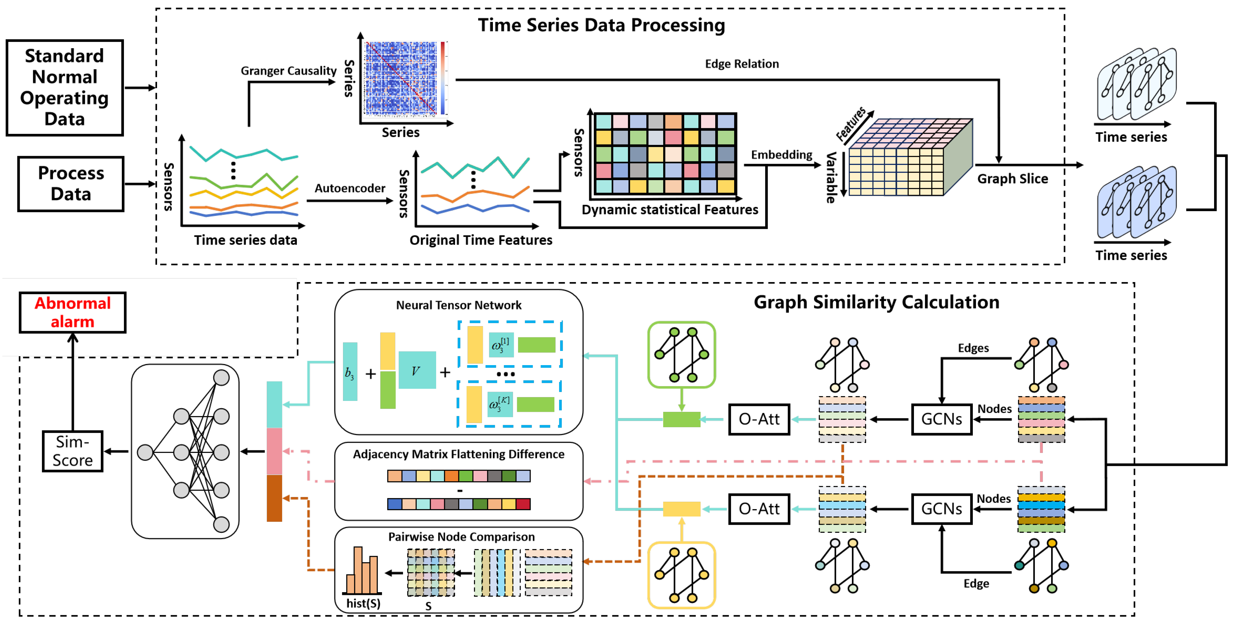
The time series anomaly monitoring model of the graph similarity network based on multi-scale features consists of two parts—the time series data processing module and graph similarity calculation module—and the model structure is shown in Figure 1. The time series data processing module takes two sets of time series data from standard normal working conditions and the monitoring process as input and completes the transformation from two-dimensional time series data to graph time series set through the multidimensional time-varying feature graph embedding process; the graph similarity computation module takes the above two sets of graph time series sets as input and obtains the similarity scores of the two graph structures in the same moment after a series of feature extraction and aggregation processes, and then converts them into graph differences to complete the process anomaly monitoring and alarm.

The multidimensional time-varying features proposed in this paper are defined as the historical data based on the moment t. The length of the time window is taken as m. The combination of the original time features of the data at the moment $\left\{t-n,t-n-1,\cdots ,t-1\right\}$ and the statistical features of the time series data computed based on the original time features are extracted as the feature representation of the data values of t at the current moment, and the multidimensional time-varying feature embedding is repeated for t as t progresses step by step in the time series, until t is the current moment. The graph structure usually consists of nodes, edges, edge weights, node features, and other elements. When mapping industrial process data into the graph space, each industrial sensor can be represented as a node in the graph structure, and the coupling relationship or physical connection between sensors can be treated as an edge connected to the node.

Complex industrial processes with dynamic and non-stationary features generate multi-dimensional spatio-temporal coupled time series data with high time dependence, based on which this paper proposes a time series data processing module to deeply extract the time dependence of the data, and at the same time, utilizes the graph structure to capture the spatial coupling relationship among sensors, and then monitors the process anomalies in a timely and accurate manner through graph similarity computation. Specifically, firstly, in the time series data processing module, Granger causality calculation is used to determine the dynamic dependency relationship among sensors, while data downscaling technology is used to construct a low-dimensional space; furthermore, a multidimensional time-varying feature map embedding strategy is adopted to expand the time series data in the two-dimensional space to the three-dimensional space and eventually mapped to the graph space, completing the graph structure of the multidimensional spatio-temporally coupled time series data. The graph structure provides a more intuitive expression for the visualization of data relationships, and at the same time, the graph space data can effectively capture the nonlinear coupling relationship between variables, thus enhancing the generalization ability and prediction accuracy of the model. Second, in the graph similarity computation module, node features of the graph structure are extracted using graph convolutional network aggregation to make them globally relevant. Further, global features at the graph level and local features at the node level are captured, respectively, using Neural Tensor Networks and histogram statistics, and are inputted to the fully connected layer for similarity score output through feature aggregation. Through the multi-level feature capture, feature aggregation, and fusion mechanism, the global structure and local details of the graph can be considered comprehensively, which significantly improves the accuracy and robustness of graph similarity calculation. In the absence of a large number of data anomaly markers, the model realizes unsupervised monitoring of industrial process anomalies by outputting the deviation score of the current production process from the standard normal production conditions as the basis for judging the anomalies. The model shows significant advantages in dealing with complex industrial process multidimensional spatio-temporal coupling time series data anomaly monitoring, which can effectively deal with complex industrial data, improve the accuracy and robustness of anomaly detection, and at the same time has a strong generalization ability, which is applicable to a variety of industrial scenarios. The overall algorithmic flow of the model is detailed in [Algorithm 1]. Through the combination of global and local features, the module can reflect the operating status of the system more comprehensively and provide reliable support for anomaly monitoring.

3.1. Time Series Data Processing

When dealing with multidimensional spatio-temporally coupled time series data of industrial processes, data dimensionality reduction and compression is a key step to improve the computational efficiency due to data redundancy and complexity. In this paper, the initially collected industrial sensor time series data are firstly represented as a set $S_{\mathrm{N}}=\{S_1,S_2,\cdots ,S_{\mathrm{n}}\}$. In order to reveal the potential dynamic linkages between sensors, the mutual information approach was first utilized to identify the complex coupling relationships between different variables in the time series that comprise the target variables for model prediction. Secondly, Granger causality analysis was used to explore the causal dependencies among the sensors. Next, an autoencoder is used to downscale the data. By minimizing the error between the input data and the reconstructed data, the self-encoder is able to learn an efficient low-dimensional representation of the data while capturing the nonlinear relationships in the data, thus retaining the key information in complex industrial data more effectively. By analyzing the distribution of potential spatial features and their contribution to the reconstruction error, sensor data that play a key role in the dimensionality reduction process can be identified, providing a more robust feature representation for subsequent anomaly detection.

The time-series causality analysis reveals the dynamic dependencies between sensor data, while the autoencoder helps to identify the variables that have a major influence by quantifying the contribution of each sensor data. Combining these methods can reduce the dimensionality of the data while retaining key information, thus improving the efficiency and accuracy of the subsequent analysis. The specific calculation formula is shown below:

$$\begin{array}{c}\hfill \mathrm{Granger}\mathrm{Causality}:{\mathbf{Y}}_{\mathrm{t}}={\beta }_0+\sum _{i=1}^p{\beta }_i{\mathbf{Y}}_{t-i}+\sum _{j=1}^{\mathrm{q}}{\gamma }_j{\mathbf{X}}_{t-j}+{\epsilon }_{2t}.\end{array}$$

(11)

$$\begin{array}{c}\hfill \mathrm{Autoencoder}\mathrm{Equation}:\stackrel{⌢}{\mathbf{X}}=f_{decoder}\left(f_{encoder}\right(\mathbf{X}\left)\right)\end{array}$$

(12)

.

By processing the industrial process sensor data, the first k main variables calculated by the autoencoder are calculated and the sorted first k sensor data are selected for normalization based on the contribution of the respective variables as the time series dataset ${\mathbf{S}}_K=\{S_1,S_2,\cdots ,S_k\}$ of the industrial process, where $k<n$, $S_i$ are the time series data of the sensor i.

For the t-moment data of $S_i$, the time window length $m=10$ is taken, and the original temporal features and statistical features of the time series data at the moment of $(S_i^{t-10},S_i^{t-9},\cdots ,S_i^{t-1})$ are used as the feature representation of the moment t. Multi-temporal dynamic feature embedding is repeated for t as t progresses step by step in the time series, so that the original time series data are extended to the three-dimensional space. The moment t data of $S_i$ embedded with dynamic multitemporal features can be expressed as

$${\mathbf{S}}_i^t=[{\mu }_i^t,Media{n}_i^t,Mod{e}_i^t,Ma{x}_i^t,Mi{n}_i^t,Q{1}_i^t,Q{2}_i^t,Q{3}_i^t,S_i^{t-1},S_i^{t-2},\cdots ,S_i^{t-10}].$$

(13)

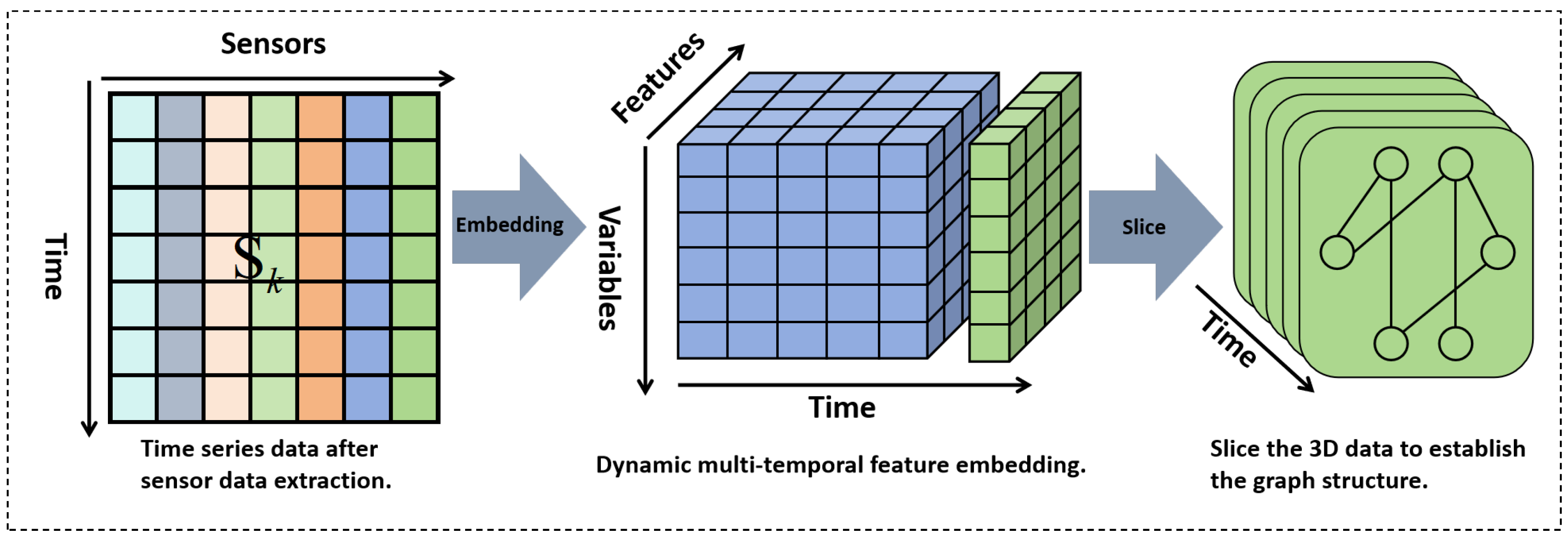
Multidimensional time-varying features are an effective structure for time domain oriented data processing, which can accurately capture the dependency and dynamic fluctuation of data on time series. The multidimensional time-varying feature graph embedding process proposed in this paper is shown in Figure 2.

The core of multidimensional time-varying feature graph embedding lies in mapping two-dimensional spatio-temporal data into the graph structure space, and constructing graph structures reflecting the system state at the current moment for the data in each time window. These time-ordered graph slices are concatenated through the time dimension to form a dynamic graph sequence, thus completely characterizing the spatial coupling properties and temporal evolution laws of sensor networks in industrial processes. This graph structure-based modeling approach has significant advantages: in the spatial dimension, the graph structure can effectively capture the complex correlations among sensors; in the temporal dimension, the dynamic graph sequence can accurately describe the state evolution of the system. By combining the theories and methods of graph theory and graph neural networks to characterize the macroscopic behavioral patterns and microscopic fluctuation characteristics of industrial data, it provides a powerful tool for the analysis and modeling of complex industrial systems.

3.2. Graph Similarity Calculation

In this section, the graph similarity calculation is described in detail. This includes the multidimensional spatial and temporal coupling of the industrial process of the standard normal operating conditions of the graph time series set and online monitoring data after time series data processing from the two-dimensional space mapped to the graph space, and the formation of graph time series set ${\mathbf{G}}_1=\{G_1^{t-n},G_1^{t-n-1},\cdots ,G_1^t\}$, ${\mathbf{G}}_2=\{G_2^{t-n},G_2^{t-n-1},\cdots ,G_2^t\}$, where ${\mathbf{G}}_1^i=(\mathbf{V},\mathbf{E})$, ${\mathbf{G}}_2^i=(\mathbf{V},\mathbf{E})$ denotes the graph structural data at the moment, including the nodes, node multidimensional time-varying features, edges, and other graph attributes. $G_1^i,G_2^i$ is used as the module input, and the graph convolutional network is used to reaggregate all node features based on neighboring nodes to obtain a new node multidimensional time-varying feature representation with global attributes, which is calculated as follows:

$$\begin{array}{c}\hfill conv\left({\mathbf{u}}_n\right)=f_1\left(\sum _{m\in N\left(n\right)}{\displaystyle \frac{1}{\sqrt{d_n{d}_m}}}{\mathbf{u}}_m{\mathbf{W}}_1^{\left(l\right)}+{\mathbf{b}}_1^{\left(l\right)}\right),\end{array}$$

(14)

where ${\mathbf{u}}_n\in {\mathbb{R}}^D$, $N\left(n\right)$ is the set of first-order neighbors of node n plus n itself, $d_n$ is the degree of node n plus 1, ${\mathbf{W}}_1^{\left(l\right)}\in {\mathbb{R}}^{D^l\times D^{l+1}}$ is the weight matrix associated with the l-th GCN layer, $b_1^{\left(l\right)}\in {\mathbb{R}}^{D^{l+1}}$ is the bias term, and $f_1(·)$ is an activation function such as $\mathrm{Re}\mathrm{LU}\left(\mathrm{x}\right)=\max (0,\mathrm{x})$.

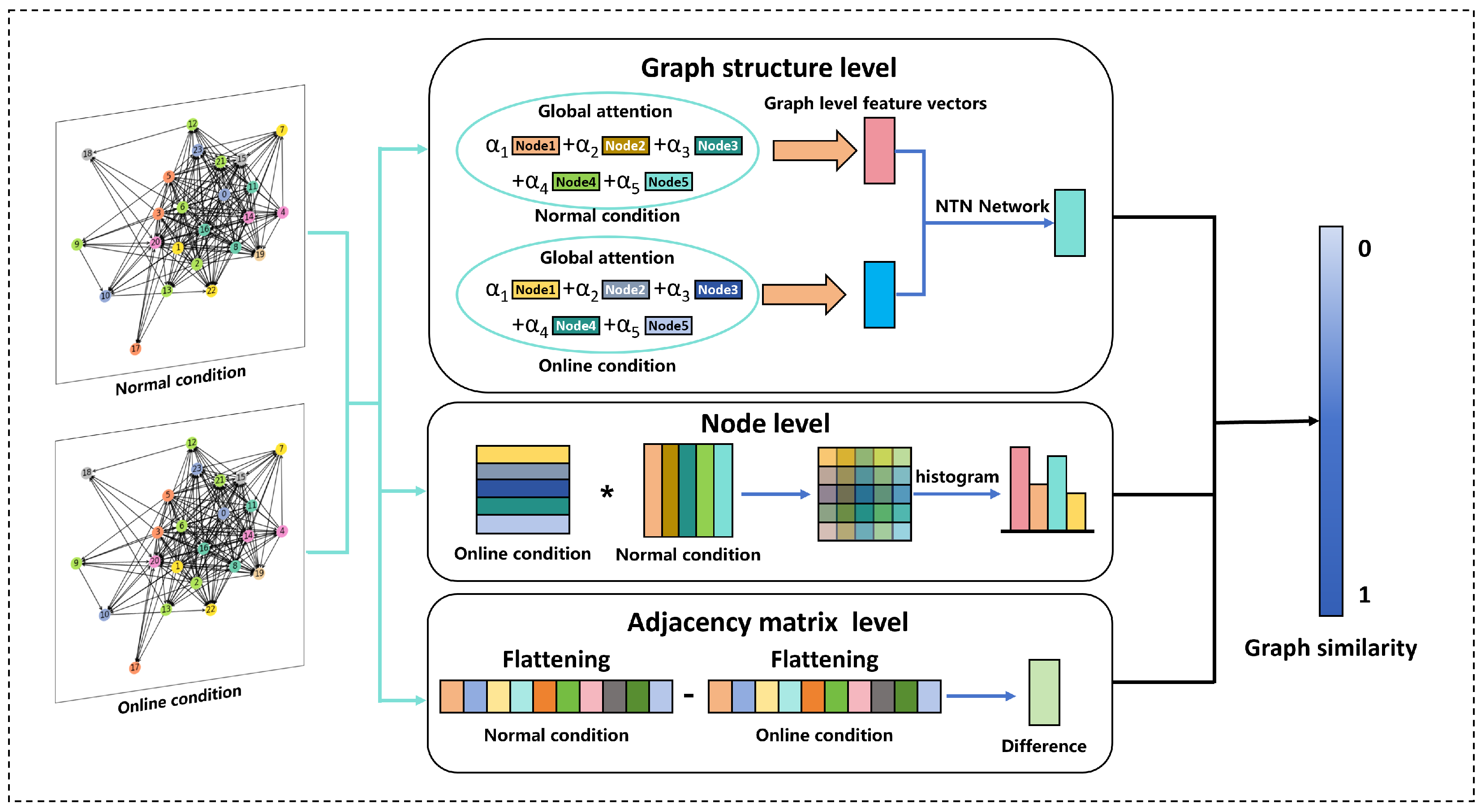
Overall, the graph convolution operation aggregates features from the first-order neighbors of a node, and when multiple graph convolution operations are performed, each node then has a feature representation of the global attributes. The graph similarity computation process after aggregation by GCN features is schematically shown in Figure 3.

3.2.1. Graph-Level Feature Aggregation

The graph-level feature aggregation can encode the structure and feature information of the graph, and through the aggregation of two graph level features, it can provide an important basis for judging the similarity between two graphs. In the initial stage of the graph similarity computation module, shown in Figure 1, different colors denote different node features, and after GCN, the node features are reaggregated and the colors are changed accordingly. After the graph structure has gone through multiple layers of GCN (three layers are taken in this paper), the node embeddings are ready to be fed into the Global Attention Awareness module (O-Att). In order to characterize each graph structure using a set of features, a weighted aggregation of the nodes’ features can be used. Therefore, in order to determine which nodes are more important and should receive more weights, we propose the Global Attention Awareness Module that allows the model to learn weights guided by a specific similarity metric.

The input node multidimensional time-varying features are represented as $U\in {\mathbb{R}}^{N\times D}$, where the nth row $u_n\in {\mathbb{R}}^D$ is the multidimensional time-varying feature representation of node n. First, compute the simple global average vector $c\in {\mathbb{R}}^D$ of the node features in the graph; then, perform a nonlinear transformation as follows:

$$\begin{array}{c}\hfill c=tanh\left(\left({\displaystyle \frac{1}{N}}\sum _{n=1}^N{\mathbf{u}}_n\right){\mathbf{W}}_2\right),\end{array}$$

(15)

where $W_2\in {\mathbb{R}}^{D\times D}$ is a learnable weight matrix. The global average vector C adaptively computes an attention weight for each node for the similarity measure of the global structural features of the graph by learning the weight matrix. For node n, take the inner product between the global average vector c and its node features, and the inner product result is used to decide that nodes that are similar to the global average vector should receive higher attention weights. Finally, the sigmoid function $\sigma \left(x\right)={\displaystyle \frac{1}{1+exp(-x)}}$ is applied to the above computed results to ensure that the attention weights are within the range (0, 1). Finally, the graph-level feature aggregation result H is the weighted sum of all node features. The above attention mechanism can be expressed as follows:

$$\begin{array}{c}\hfill \mathbf{h}=\sum _{n=1}^N{f}_2\left({\mathbf{u}}_n^T\mathbf{c}\right){\mathbf{u}}_n=\sum _{n=1}^N{f}_2\left({\mathbf{u}}_n^{T}tanh\left(\left({\displaystyle \frac{1}{N}}\sum _{m=1}^N{\mathbf{u}}_m\right){\mathbf{W}}_2\right)\right){\mathbf{u}}_n,\end{array}$$

(16)

where $f_2(·)$ is the sigmoid function $\sigma (·)$.

The weighted graph-level feature aggregation result $h_i,h_j$ is thus obtained for modeling the relationship between two graph-level embeddings using a neural tensor network (NTN):

$$\begin{array}{c}\hfill \vartheta ({\mathbf{h}}_i,{\mathbf{h}}_j)=f_3\left({\mathbf{h}}_i^T{\mathbf{W}}_3^{[1:K]}{\mathbf{h}}_j+\mathbf{V}\left[\begin{array}{c}{\mathbf{h}}_i\hfill \\ {\mathbf{h}}_j\hfill \end{array}\right]+{\mathbf{b}}_3\right),\end{array}$$

(17)

where $W_3^{[1:K]}\in {\mathbb{R}}^{D\times D\times K}$ is the weight tensor, $\left[ \right]$ denotes the tandem operation, $V\in {\mathbb{R}}^{K\times 2D}$ is a weight vector, $b_3\in {\mathbb{R}}^K$ is a bias vector, $f_3(·)$ is an activation function, K is a hyperparameter, and the control model is the number of interaction (similarity) scores generated for each graph embedding pair.

3.2.2. Comparison of Node-Level Features

Node-level information (e.g., node feature distributions and graph sizes) may be lost as a result of computing graph-level feature aggregation. In graph sequence data of industrial processes, the key to the difference between two graphs lies in the difference in node features, which is often difficult to reflect by graph-level features. Therefore, node-level feature comparison is also a key part of the process of computing graph similarity.

The pairwise interaction score between nodes is calculated by the following equation:

$$\begin{array}{c}\hfill S=\sigma \left({\mathbf{U}}_i{\mathbf{U}}_j^T\right),\end{array}$$

(18)

where $U_i\in {\mathbb{R}}^{N_i\times D}$, $U_j\in {\mathbb{R}}^{N_j\times D}$ is the characteristic representation of node i and node j. Since the node-level features are not normalized, a Sigmoid function is applied to ensure that the similarity score is in the range (0, 1). In order to ensure that the model’s representation of the graph structure is invariant, a more efficient and natural way of utilizing S needs to be considered. Therefore, it is taken to extract its histogram feature: $hist\left(s\right)\in {\mathbb{R}}^B$, where B is the hyperparameter (in this paper, $B=16$) that controls the bins in the histogram. The histogram feature vector, denoted as $\varsigma$, is normalized and output as a key part of the graph similarity computation.

3.2.3. Difference Computation After Adjacency Matrix Spreading

After obtaining the graph-level features and node differences, we focus our attention on the adjacency matrix in order to capture the more detailed differences between the two graphs. The adjacency matrices of the two graphs are flattened into one-dimensional vectors, where each element denotes the degree (i.e., the number of neighbors) of the corresponding node. Specifically, for graphs $G_1$ and $G_2$, their adjacency matrices are ${\mathbf{A}}_1$ and ${\mathbf{A}}_2$, respectively, where ${\mathbf{A}}_1,{\mathbf{A}}_2\in {\mathbb{R}}^{n\times n}$, and n is the number of nodes. First, calculate the degree vector for each node: ${\mathbf{D}}_1={\left[{\displaystyle \sum _{j=1}^n}{\mathbf{A}}_{1,ij}\right]}_{i=1}^n$, ${\mathbf{D}}_2={\left[{\displaystyle \sum _{j=1}^n}{\mathbf{A}}_{2,ij}\right]}_{i=1}^n$. Then, the values of the corresponding positions of these two degree vectors are subtracted to obtain a new vector:

$$\begin{array}{c}\hfill {\Delta }_D={\mathbf{D}}_1-{\mathbf{D}}_2,\end{array}$$

(19)

where the length of ${\Delta }_D$ is the number of nodes n and each element represents the difference between the degrees of the corresponding nodes in the two graphs.

Through the above calculation, the difference relationship between the neighboring matrices of two graphs is obtained more intuitively, which provides the basis for graph similarity calculation.

3.2.4. Similarity Score Calculation and Exception Alarm

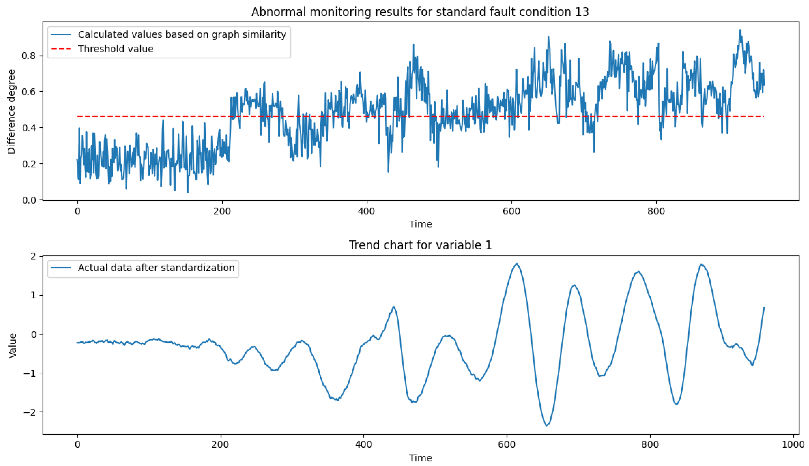
The coarse global information from graph-level feature aggregation is combined with the fine-grained information captured by node-level feature comparisons as well as the difference features of the adjacency matrix in order to provide a comparative, comprehensive graph structure characterization of the model. In the final stage, a standard multi-layer fully connected neural network is applied to gradually reduce the dimensionality of the similarity score vector. Finally, a score ${\stackrel{⌢}{s}}_{ij}$ ∈ R is predicted and compared to the ground truth similarity score using the following mean square error loss function:

$$\begin{array}{c}\hfill \zeta ={\displaystyle \frac{1}{\left|\vartheta \right|}}\sum _{(i,j)\in \vartheta }({\stackrel{⌢}{s}}_{ij}-s(G_1^i{G}_2^i))\end{array},$$

(20)

where $\vartheta$ is the set of training graph pairs and $s\left(G_1^i{G}_2^i\right)$ is the true similarity between $G_1^i,G_2^i$, obtained by normalizing the Euclidean distance of the node vectors:

$$\begin{array}{c}\hfill s\left(G_1^i{G}_2^i\right)=Normalization\left(d\left(G_1^i{G}_2^i\right)\right),\end{array}$$

(21)

where $d\left(G_1^i{G}_2^i\right)=\sqrt{{\displaystyle \sum _{k=1}^n}{(p_k-q_k)}^2}$ is the Euclidean distance formula; $p_k,q_k$ denotes the coordinate values of node p and node q in the kth dimension, respectively; and n denotes the number of dimensions of the space.

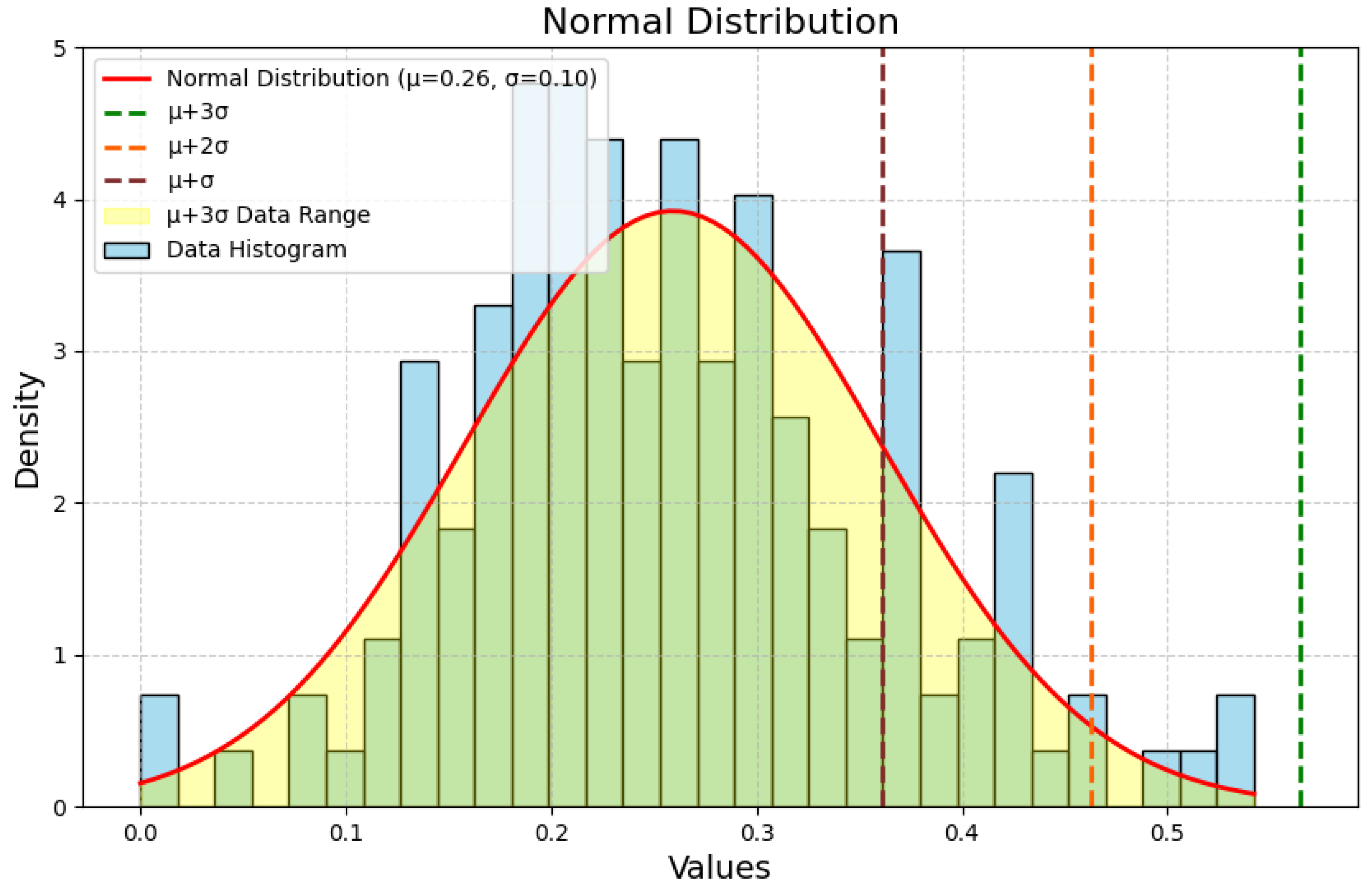
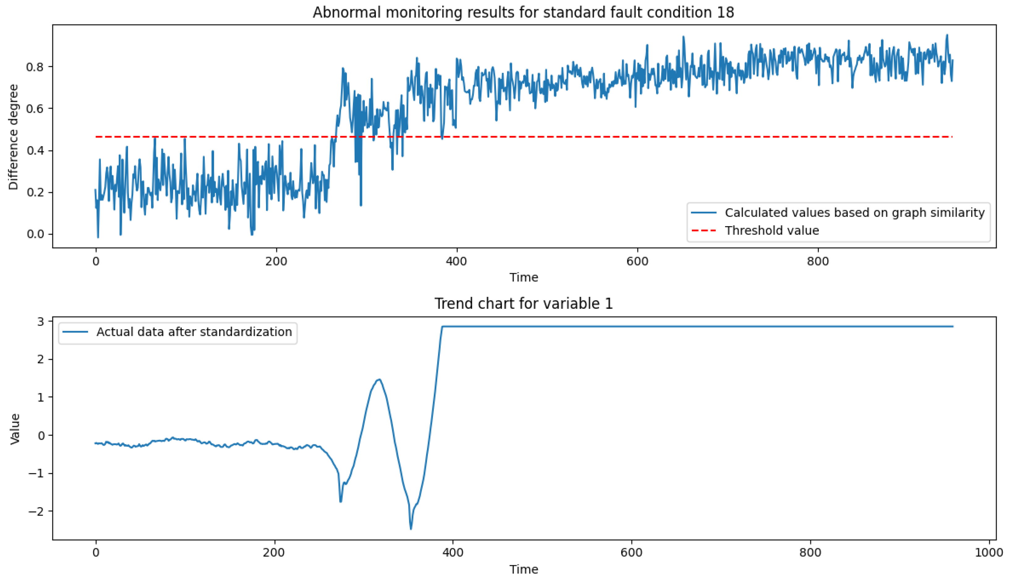
The calculated similarity score ${\stackrel{⌢}{s}}_{ij}$ ∈ R transformed into the difference score between [0, 1], with larger values indicating larger differences. Analyze the distribution of the data variability under normal operating conditions and transform it into a normal distribution, and select $\mathit{\mu }+3\mathit{\sigma }$ of the variability distribution under normal operating conditions as the threshold for anomaly monitoring. The implementation process is described in Section 4.2.1. By comparing the deviation of the difference score calculated by the model with the overrun threshold, the abnormal state at the current moment is determined.

3.3. Application Steps

This section summarizes about the process algorithms and application steps proposed in this paper, detailed process analysis as [Algorithm 1].

Algorithm 1 Anomaly monitoring model of industrial processes based on graph similarity and applications.

Require:  1.  $S_{st}=\{S_1,S_2,\cdots ,S_n\}$: Standard normal operating conditions time series data.  2.  $S_{online}=\{S_1,S_2,\cdots ,S_n\}$: Online monitoring of time series data.  3.  m: The length of the time window. Ensure:  1.  Trained model.  2.  Graph Discrepancy Score.  3.  Abnormal Alarms. 1: Initialize the time window and graph model. 2: (1) Offline Modeling: 3: 1. Preprocessing: 4: Granger causality and mutual information were applied to calculate the coupling between variables. 5: Apply Autoencoder to reduce dimensionality of $S_{st},S_{online}$, resulting in $S_{k1},S_{k2}$. 6: 2. Multidimensional time-varying feature graph embedding: 7: for each time step t in $\mathrm{T}$ do 8:     if $t\ge 10$ then 9:         for each sensor i in $S_{k1},S_{k2}$ do 10:            Feature1 = $\{S_{\mathrm{i}}^{t-10},S_{\mathrm{i}}^{t-9},\cdots ,S_{\mathrm{i}}^{t-1}\}$ 11:            Feature2 = statistics($\{S_{\mathrm{i}}^{t-10},S_{\mathrm{i}}^{t-9},\cdots ,S_{\mathrm{i}}^{t-1}\}$) 12:            Feature = concat[Feature1, Feature2] 13:            ${Graph}^t$ = $Data$ (Feature, [$Granger\_causalit{y}_{i,j}^t$]) 14:         end for 15:     else 16:         continue 17:     end if 18: end for 19: 3. Model Training: 20:    Train the Model using Graph_set. 21:    Label = Euclidean distance(Nodes) 22:    Graph Similarity Calculation 23: (2) Online anomaly monitoring and location tracing: 24:    Online monitoring data preprocessing. 25:    Apply the trained model to compute graph similarity. 26:    Comparison of graph similarity calculations with overrun thresholds.

Note:

• $S_i^t$: Data of sensor i at time t.
• $S_K$: Sensor data after dimensionality reduction.
• Feature1: Raw time characteristics of dynamic data.
• Feature2: Dynamic statistical characteristics of dynamic data.
• Feature: Multidimensional time-varying characteristics of time series data.
• ${Graph}^t$: Graph structure of data at time t.
• Graph_set: A set of graph sequences after time series data are mapped to graph space.

4. Experimental Applications

This section validates the validity and reliability of the application of the graph similarity network time series anomaly monitoring model based on multi-scale features proposed in this paper based on Tennessee-Eastman (TE) process data. The dataset used and a discussion of the experimental results are presented in the following section.

4.1. Introduction to the Tennessee-Eastman (TE) Process Dataset

Based on the actual chemical reaction process, Eastman Chemical Company has developed an open and challenging chemical modeling simulation platform, the Tennessee-Eastman (TE) simulation platform. The data generated by this platform are time-varying, strongly coupled, and nonlinear, and they are widely used to test control, monitoring, and troubleshooting models of complex industrial processes. A schematic diagram of the TE process is shown in Figure 4.

The TE process dataset consists of a training set and a test set, and the training set and test set data consist of data from 22 different simulation runs, respectively, with each sample datum containing 12 manipulated variables, 22 continuous process measurement variables, and 19 component measurement variables. The training set samples are numbered as d00.dat to d21.dat, and the test set samples are numbered as d00_te.dat to d21_te.dat, where d00.dat and d00_te.dat are the samples under normal operating conditions. d00.dat training samples are obtained under 25 h running simulation. The total number of observations is 500; d00_te.dat test samples were obtained under 48 h running simulation and the total number of observations is 960. d01.dat to d21.dat are training set samples with faults and d01_te.dat to d21_te.dat are test set samples with faults. Each sample in the training set∖test set represents a fault, where the training set samples with faults were obtained under a 25 h running simulation. The simulation starts without faults and faults are introduced at the 1 h moment of the simulation time, but the observations are collected only after the introduction of the faults, i.e., there are only 480 observations. The test set samples with faults were obtained under a 48 h running simulation; the faults were introduced at the 8 h time moment and a total of 960 observations were collected, of which the first 160 observations were normal data.

4.2. Experimental Analysis and Discussion of Results

4.2.1. Experimental Modeling

Considering the diversity of normal operating conditions data distribution, the combination of normal operating conditions time series data and some fault conditions time series data in the dataset is used as the training set to model and train the model.

Mutual information is a statistical tool used to quantify the correlation between two variables, which reveals the extent to which information about one variable can be predicted or understood when information about the other variable is known. Thus, the use of mutual information can quantify the nonlinear relationship between two variables and help identify the information transfer relationship between them. Granger causality was used to determine the causal relationship between the sensors selected by the above process. Specifically, we first utilize the mutual information between variables as a screening tool to identify groups of variables with strong coupling relationships and construct an undirected graph structure based on it. Mutual information can capture the global nonlinear dependencies between variables and is suitable for high-dimensional and nonlinear data, thus ensuring that the graph structure can comprehensively reflect the coupling strength between variables. Next, we optimize the undirected graph structure to a directed graph structure by calculating the causal relationship between the above variables with connectivity through Granger causality. Granger causality is able to capture the dynamic causality in the time series, which further enhances the accuracy of the graph structure. The advantage of this approach is that it can significantly improve the accuracy and robustness of anomaly detection. First, the introduction of mutual information ensures that the graph structure can comprehensively capture the nonlinear dependencies among variables, while the optimization of Granger causality further enhances the accuracy of the graph structure. Second, by filtering the strong coupling relations and optimizing the directed edges, the noise interference can be effectively filtered and the robustness of the model in the noisy environment can be enhanced. In addition, the method is highly generalized and scalable, providing a more effective solution for data compression and dimensionality reduction in industrial process anomaly monitoring. A maximum lag order of nine was chosen, and the relationship test was selected as residual squared and F-test with a p-value less than 0.05, and this was used as the edge of the connection between the nodes. The causality results are shown in Figure 5.

Dimensionality reduction and data compression operations on sensor datasets using autoencoder. The selection of potential dimensions with a cumulative explanatory power of 80% of the autoencoder reconstruction error and the eventual selection of 24 sensor variables as key features that can effectively characterize industrial processes significantly reduces the dimensionality of the data. The selection results are shown in Figure 6 and

Table 1. Results of the TE process autoencoder extraction of sensor variables, numbered in order of largest to smallest explained variance ratios.

Node Number	Sensor Number	Sensor Name
0	44	Total feed volume
1	6	Reactor pressure
2	18	Stripper Steam Flow
3	36	Product component D
4	7	Reactor level
5	28	Reactor feed component C
6	29	Empty material component A
7	1	Material D Flow
8	45	Compressor recirculation valve
9	25	Reactor feed component D
10	19	Compressor power
11	15	Stripper pressure
12	48	Stripper gas flow
13	14	Stripper Level
14	51	Condenser cooling water flow
15	39	Product component G
16	26	Reactor feed component E
17	41	D feed volume
18	27	Reactor feed component F
19	10	Vapor/liquid separator temperature
20	12	Vapor/liquid separator pressure
21	32	Empty material component E
22	34	Empty material component G
23	49	Steam Valve for Stripper Tower

.

From the above Granger causality calculation results and with reference to expert experience, a multidimensional time-varying feature graph embedding work is carried out based on the main influencing variables in the downscaling results of the autoencoder data, which extends the two-dimensional time-series data to the three-dimensional space, and then maps them to the graph space, so as to establish a set of graph sliced sequences based on the multi-temporal features, where each layer of the graph structure is schematically shown in Figure 7.

The industrial condition data from the TE dataset are individually built into a set of graph slice sequences based on multi-temporal features according to the above steps. The proposed industrial process anomaly monitoring model based on graph similarity computation takes two time series sets of the same length as inputs; feeds the stable graph slice sequence set into the model for offline training; and retains the better model parameters to complete the online monitoring task on process data after training, where the inputs for the online monitoring task are the standard normal working condition data and online data. The Loss curve of offline model training is shown in Figure 8.

The distribution of the degree of variability of the data under normal operating conditions was analyzed and transformed into a normal distribution, the results of which are shown in Figure 9.

The red curve in the figure shows the distribution of normalized variability under normal working conditions, and the brown, orange, and green vertical lines are the positions of $\mu +\sigma$, $\mu +2\sigma$, and $\mu +3\sigma$, respectively. In the normal distribution, about 99.7% of the data fall within the range of $\mu +3\sigma$, while in industrial production, $\mu +3\sigma$ is known as the control limit that is often used for anomaly identification. In the distribution of the degree of variation of normal operating conditions for the dataset used in this paper, $\mu +3\sigma$ covers almost 100% of the data and is, therefore, more representative. Thus, in the revised manuscript, we chose $\mu +3\sigma$ for the distribution of the degree of variability of normal operating conditions as the threshold for anomaly monitoring. In all proposed responses, we used $\mu +3\sigma$ as the threshold for anomaly monitoring to complete the experimental analysis.

4.2.2. Anomalous Monitoring Results

After analyzing the TE process fault samples, it is concluded that fault condition 01 is a step-steady state change, which can characterize the actual production conditions of the process transient anomalies, such as the material changes to correct the re-entry of the steady state; fault condition 06 is a step change, which can be characterized by sudden-type faults in actual production conditions, such as mechanical failures, steep pressure increases, etc.; fault condition 13 is a sinusoidal change, which can characterize slow-change faults in actual production conditions, such as slow drift in sensor accuracy, pipe leakage, etc.; fault condition 18 contains both step and sinusoidal, two types of process parameter changes. Therefore, this paper selects the test set data of fault conditions 01, 06, 13, and 18 (data length of 960) as the validation dataset to verify the reliability of the model proposed in this paper. Figure 10, Figure 11, Figure 12 and Figure 13 show the anomaly monitoring of the above faulty working conditions by the proposed model in this paper, respectively. The upper part of the figure shows the comparison of the discrepancy monitoring value and the threshold value between the faulty condition and the normal condition, where the blue line represents the real-time monitoring value of the discrepancy and the orange line represents the over-limit threshold value; the lower part is the standardized result of variable 1 under the condition, and the combination of the two parts can accurately reflect the trend of the process data over time and the anomalous situation. Due to the hysteresis of industrial processes, after injecting faults into the system, the anomalies propagate slowly in the industrial topology; further, after a period of time, the anomalies occur slowly in a trend similar to the change of slopes, and the model responds quickly and sends out an anomaly alarm when the set threshold is exceeded.

Figure 10 demonstrates the anomaly monitoring of the model proposed in the article for the standard fault condition 01. In this case, variable 1 shows a sinusoidal oscillatory trend at moments 160–500, followed by a steady state at moments 500–960. The anomaly monitoring results show that in the 160–500 moments of abnormal fluctuations in process data to the upper and lower peaks of the graph, variance reaches its maximum and the model reacts to it; then, in the process of convergence to the steady state, the variance will gradually decrease and fall back to within the threshold line of the overrun limit, in which there are still small fluctuations in the process data, and the model quickly senses and monitors the changes in the graph variance.

Figure 11 shows in detail the monitoring results for faulty condition 06. Before the fault is injected (moments 0–160), the discrepancy variance value maintains at a normal level and fluctuates slightly following the change of variables. After the fault is injected at moment 160, the discrepancy monitoring value changes with the system step change and remains abnormal thereafter, clearly indicating the sensitive response of the model to the fault. It is worth noting that despite the fault being injected at moment 160, the model’s detection value does not change immediately, and it is not until about moment 210 that the model’s prediction changes significantly. This delay phenomenon can be explained by analyzing the system response at the initial stage of fault injection. At the initial stage of fault injection, the macroscopic performance of the whole industrial process does not change significantly and immediately, despite the change detected by the sensors of variable 1, which is consistent with the system inertia in the real production process. After about 280 moments, the value of variable 1 reaches a new stable level and remains stable thereafter. The maintenance of this stabilization period suggests that once the system has adapted to the faulty state, its behavior will stabilize until appropriate corrective actions are taken. The model proposed in this paper is able to deeply extract the temporal and spatial coupling of production data and is able to capture and issue timely alarms in case of process anomalies, which is of great practical application value for improving the reliability and safety of industrial processes.

In an in-depth analysis of the standard fault condition 13, we observed that after the introduction of the fault in the system at the moment of time point 160, the production data started to exhibit significant non-stationary sinusoidal oscillatory characteristics and this oscillatory pattern contrasted with the stable or cyclic variation trend that the system exhibits under normal operating conditions. Over time, the amplitude of data oscillations under faulty conditions gradually increases due to the drift of key reaction dynamics parameters, showing a continuous change in the dynamic characteristics of the system. By comparing the sequence of data plots under abnormal conditions and standard normal conditions, it can be found that the difference between the two shows a trend of gradual increase accompanied by oscillation, and when the oscillation falls back to the normal region, the difference between the conditions also decreases. The model accurately identifies and follows the abnormal changes between the conditions and quantifies them as difference scores, which provides a reliable basis for monitoring the anomalies.

The experimental results for the standard fault condition 18 are shown in Figure 13. In an exhaustive analysis of the anomaly monitoring results for the standard fault condition 18, by looking at the trend plot of variable 1, we find that after the introduction of the fault, the data undergo a half-sinusoidal variation followed by a significant jump and then stabilize. Characterizing anomaly changes using the degree of dissimilarity means that the magnitude of the dissimilarity value varies with the fluctuation of the anomaly over time, and when the anomaly variable remains stable, the degree of dissimilarity between the cases also remains stable within a certain range because the graph similarity calculation is oriented towards the influence of global variables with spatio-temporal coupling relationships.

4.2.3. Control Experiments

In this paper, three groups of controlled experiments are set up to verify the effectiveness of the proposed model. The first group is a control experiment of anomaly monitoring based on the data of standard fault condition 01 using the traditional cosine similarity calculation method in the form of similarity measure with the model proposed in this paper. The second group is a control experiment of anomaly monitoring based on the data of standard fault condition 01 using the PCA through the multivariate statistics of the over-limit determination method with the model proposed in this paper. The third group is a control test using traditional statistical and deep learning methods based on data from standard fault conditions 06, 13, and 18, with FNR and FPR as benchmarks, against the model proposed in this paper. The experimental results are shown below.

In the first set of control experiments, the anomaly detection method based on cosine similarity is used to analyze the process data of standard anomaly condition 01. Specifically, we converted the cosine similarity results for each time point into a difference degree value in the interval [0, 1], where a larger difference degree value indicates a more significant difference between the data at the two time points. Figure 14 illustrates the results of this experiment, where the red scatter marks the detected anomalies, the red dashed line indicates the preset threshold line, and the blue curve depicts the trend of the degree of dissimilarity over time. In this experiment, 80% of the cosine similarity is set as the overrun threshold and converted to the value of the dissimilarity in the interval [0, 1]. Through Figure 14, it can be observed that the traditional cosine similarity-based anomaly detection method shows significant limitations in complex industrial process data, mainly in the form of higher false alarms and omissions, while there is no significant difference between normal and anomalous data. Specifically, in the range of 200 to 960 time points, the system incorrectly marks some normal data points as abnormal, indicating that the cosine similarity calculation method fails to adequately capture the local features and global coupling relationships of the data. Meanwhile, some of the actual abnormal data points are not effectively identified, further revealing that the method is difficult to accurately capture the abnormal signals in industrial data with strong spatio-temporal coupling relationships. This experiment demonstrates the limitations of the traditional similarity calculation method in dealing with complex industrial process data.

The results of the second set of control experiments are shown in Figure 15, which demonstrates the results of monitoring the squared prediction error (SPE) statistic of PCA for standard abnormal operating condition 01. During the training of the PCA model, it was determined through several experiments that 80% of the variance was retained and the reconstruction error was set to 90%. This parameter choice effectively reduces the dimensionality of the data while retaining most of the important information, thus allowing the model to achieve optimal performance. After moment point 170, the PCA model responds to the abnormalities of the industrial conditions. Although variable 1 stabilizes after the 500th moment, other variables of the overall industrial process will still be out of the normal range at some moments, which are captured by the system and labeled as abnormal states. The PCA model is able to differentiate the abnormal data to a certain extent, but there are still false alarms and omissions. Meanwhile, when observing the results of PCA in the normal state (the first 160 moments), there are still some false alarms. This result suggests that the PCA model has some limitations in dealing with the spatial coupling relationships and time dependence of the data. Specifically, PCA, as a linear dimensionality reduction method, mainly relies on the second-order statistical properties of the data (i.e., covariance matrix), which makes it difficult to adequately capture the nonlinear relationships and dynamic properties in the data, and its detection may be less than ideal. In addition, the PCA model has a high sensitivity to outliers, which may lead to an increase in false alarms. Despite the advantages of PCA in terms of dimensionality reduction and feature extraction, its limitations may lead to a decrease in the accuracy of anomaly detection when dealing with complex industrial process data and may not be able to adequately capture the nonlinear relationships and dynamic properties in the data, which may lead to poor performance in the anomaly detection task. We should explore more adaptive and better methods to address the above limitations.

The results of the third set of control experiments are shown in

Table 2. Results of the third group of controlled experiments.

Methods	PCA		CNN		LSTM		GCN		GAT		Proposed Model
Index	FNR	FPR	FNR	FPR	FNR	FPR	FNR	FPR	FNR	FPR	FNR	FPR
Test1	0.132	0.113	0.061	0.200	0.091	0.107	0.085	0.096	0.077	0.093	0.080	0.078
Test2	0.155	0.160	0.164	0.180	0.129	0.180	0.115	0.158	0.132	0.146	0.107	0.134
Test3	0.128	0.193	0.121	0.180	0.116	0.207	0.115	0.187	0.106	0.155	0.097	0.142

, which were conducted by principal component analysis (PCA), convolutional neural network (CNN), and long short-term memory network (LSTM) against the method proposed in this paper.

Table 2 systematically compares the performance of six methods (PCA, CNN, LSTM, GCN, GAT, and the method proposed in this paper) on multiple faulty conditions, focusing on evaluating two key metrics, FNR and FPR, to measure the accuracy and robustness of the model in anomaly detection tasks. The experimental data show that the model proposed in this paper (Sim-GNN) demonstrates significant performance advantages in all the tests, while achieving a good balance between FPR and FNR, both of which are at a low level.

In contrast, PCA, as a linear dimensionality reduction method, has a higher FNR (e.g., FPR of 0.132 in Test1), and the difference between FPR and FNR is more obvious, although it performs better in FPR (e.g., FPR of 0.113 in Test1). This indicates that PCA has some limitations in dealing with high-dimensional and nonlinear data, and it is difficult to adequately capture the complex structure and dynamic properties in the data. CNN and LSTM—although they perform better in local feature extraction and time-series modeling, and are able to capture long-term dependencies in time series—have deficiencies in dealing with spatially coupled data modeling with a global structure. This results in large values of its FPR and FNR, which affects the overall performance of the model in anomaly detection tasks. In addition, GCN and GAT, as graph neural network methods, outperform PCA, CNN, and LSTM in terms of FNR and FPR, but are still not as good as Sim-GNN. Despite their ability to capture spatial dependencies in the data, GCN and GAT have limitations in dealing with complex spatio-temporal coupling relationships.

In summary, the model proposed in this paper is able to better model the global structure and spatio-temporal coupling relationship in industrial processes by combining the advantages of graph neural networks, and effectively deal with temporal dependence and spatial dependence, thus achieving better performance in anomaly detection tasks. This result shows that Sim-GNN has high accuracy and robustness in dealing with complex industrial process data, providing new ideas and methods for future anomaly detection research.

5. Conclusions

In this paper, a graph similarity network time series anomaly monitoring model based on multi-scale features is proposed, while introducing a multi-dimensional time-varying feature embedding method based on historical data and a data building graph structure method based on data reduced dimensionality and causality calculation. Based on this, an inter-graph similarity calculation method by aggregating global features, node differences, and neighbor matrix differences is designed for process anomaly monitoring applications. The reliability and timeliness of the proposed method in real-world scenarios are verified by standard normal operating condition data as well as standard fault data of the Tennessee-Eastman (TE) process. The proposed method for multidimensional spatio-temporal coupling time series data, and unsupervised and accurate monitoring of abnormal conditions with fewer model parameters, effectively reduces the false alarms and omissions of normal measurement points under abnormal conditions of industrial processes and provides strong technical support for intelligent monitoring and fault diagnosis of industrial processes.

References

1. Yang, T.; Yi, X.; Lu, S.; Johansson, K.H.; Chai, T. Intelligent manufacturing for the process industry driven by industrial artificial intelligence. Engineering 2021, 7, 1224–1230. [Google Scholar] [CrossRef]
2. Liu, J.; Ren, Y. A general transfer framework based on industrial process fault diagnosis under small samples. IEEE Trans. Ind. Inform. 2020, 17, 6073–6083. [Google Scholar] [CrossRef]
3. Dai, X.; Gao, Z. From model, signal to knowledge: A data-driven perspective of fault detection and diagnosis. IEEE Trans. Ind. Inform. 2013, 9, 2226–2238. [Google Scholar] [CrossRef]
4. Ding, S.X. Data-driven design of monitoring and diagnosis systems for dynamic processes: A review of subspace technique based schemes and some recent results. J. Process Control 2014, 24, 431–449. [Google Scholar] [CrossRef]
5. Jiang, M.; Wang, K.; Sun, Y.; Chen, W.; Xia, B.; Li, R. MLGN: Multi-scale local-global feature learning network for long-term series forecasting. Mach. Learn. Sci. Technol. 2023, 4, 045059. [Google Scholar]
6. Qin, S.J. Survey on data-driven industrial process monitoring and diagnosis. Annu. Rev. Control 2012, 36, 220–234. [Google Scholar] [CrossRef]
7. Jing, C.; Hou, J. SVM and PCA based fault classification approaches for complicated industrial process. Neurocomputing 2015, 167, 636–642. [Google Scholar]
8. Ibebuchi, C.C.; Obarein, O.A.; Abu, I.O. Application of autoencoders artificial neural network and principal component analysis for pattern extraction and spatial regionalization of global temperature data. Mach. Learn. Sci. Technol. 2024, 5, 015009. [Google Scholar]
9. Zhou, P.; Zhang, R.; Xie, J.; Liu, J.; Wang, H.; Chai, T. Data-driven monitoring and diagnosing of abnormal furnace conditions in blast furnace ironmaking: An integrated PCA-ICA method. IEEE Trans. Ind. Electron. 2020, 68, 622–631. [Google Scholar]
10. Wang, X.; Kruger, U.; Lennox, B. Recursive partial least squares algorithms for monitoring complex industrial processes. Control Eng. Pract. 2003, 11, 613–632. [Google Scholar]
11. Li, Z.; Liu, F.; Yang, W.; Peng, S.; Zhou, J. A survey of convolutional neural networks: Analysis, applications, and prospects. IEEE Trans. Neural Netw. Learn. Syst. 2021, 33, 6999–7019. [Google Scholar] [CrossRef] [PubMed]
12. Jiao, J.; Zhao, M.; Lin, J.; Liang, K. A comprehensive review on convolutional neural network in machine fault diagnosis. Neurocomputing 2020, 417, 36–63. [Google Scholar] [CrossRef]
13. Yu, J.; Liu, X.; Ye, L. Convolutional long short-term memory autoencoder-based feature learning for fault detection in industrial processes. IEEE Trans. Instrum. Meas. 2020, 70, 3505615. [Google Scholar] [CrossRef]
14. Tang, Y.; Wang, Y.; Liu, C.; Yuan, X.; Wang, K.; Yang, C. Semi-supervised LSTM with historical feature fusion attention for temporal sequence dynamic modeling in industrial processes. Eng. Appl. Artif. Intell. 2023, 117, 105547. [Google Scholar] [CrossRef]
15. Mao, W.L.; Chiu, Y.Y.; Lin, B.H.; Wang, C.C.; Wu, Y.T.; You, C.Y.; Chien, Y.R. Integration of deep learning network and robot arm system for rim defect inspection application. Sensors 2022, 22, 3927. [Google Scholar] [CrossRef]
16. Liu, S.; Ni, H.; Li, C.; Zou, Y.; Luo, Y. DefectGAN: Synthetic Data Generation for EMU Defects Detection with Limited Data. IEEE Sens. J. 2024, 24, 17638–17652. [Google Scholar] [CrossRef]
17. Rao, S.; Wang, J. A comprehensive fault detection and diagnosis method for chemical processes. Chem. Eng. Sci. 2024, 300, 120565. [Google Scholar] [CrossRef]
18. Md Nor, N.; Che Hassan, C.R.; Hussain, M.A. A review of data-driven fault detection and diagnosis methods: Applications in chemical process systems. Rev. Chem. Eng. 2020, 36, 513–553. [Google Scholar] [CrossRef]
19. Dokmanic, I.; Parhizkar, R.; Ranieri, J.; Vetterli, M. Euclidean distance matrices: Essential theory, algorithms, and applications. IEEE Signal Process. Mag. 2015, 32, 12–30. [Google Scholar] [CrossRef]
20. Mussabayev, R. Optimizing Euclidean Distance Computation. Mathematics 2024, 12, 3787. [Google Scholar] [CrossRef]
21. Xia, P.; Zhang, L.; Li, F. Learning similarity with cosine similarity ensemble. Inf. Sci. 2015, 307, 39–52. [Google Scholar]
22. Zheng, L.; Jia, K.; Wu, W.; Liu, Q.; Bi, T.; Yang, Q. Cosine similarity based line protection for large scale wind farms part II—The industrial application. IEEE Trans. Ind. Electron. 2021, 69, 2599–2609. [Google Scholar] [CrossRef]
23. Atluri, G.; Karpatne, A.; Kumar, V. Spatio-temporal data mining: A survey of problems and methods. ACM Comput. Surv. (CSUR) 2018, 51, 83. [Google Scholar]
24. Li, H.; Liu, J.; Yang, Z.; Liu, R.W.; Wu, K.; Wan, Y. Adaptively constrained dynamic time warping for time series classification and clustering. Inf. Sci. 2020, 534, 97–116. [Google Scholar] [CrossRef]
25. Bai, Y.; Ding, H.; Bian, S.; Chen, T.; Sun, Y.; Wang, W. Simgnn: A neural network approach to fast graph similarity computation. In Proceedings of the Twelfth ACM International Conference on Web Search and Data Mining, Melbourne, VIC, Australia, 11–15 February 2019; pp. 384–392. [Google Scholar]
26. Sahinoglu, O.; Kumluca Topalli, A.; Topalli, I. Discovering Granger causality with convolutional neural networks. J. Intell. Manuf. 2024, 1–14. [Google Scholar] [CrossRef]
27. Geweke, J. Measurement of linear dependence and feedback between multiple time series. J. Am. Stat. Assoc. 1982, 77, 304–313. [Google Scholar]
28. Chen, Y.; Rangarajan, G.; Feng, J.; Ding, M. Analyzing multiple nonlinear time series with extended Granger causality. Phys. Lett. A 2004, 324, 26–35. [Google Scholar]
29. Zhao, C. Perspectives on nonstationary process monitoring in the era of industrial artificial intelligence. J. Process Control 2022, 116, 255–272. [Google Scholar]
30. Wang, Y.; Yao, H.; Zhao, S. Auto-encoder based dimensionality reduction. Neurocomputing 2016, 184, 232–242. [Google Scholar]
31. Zheng, S.; Zhao, J. A new unsupervised data mining method based on the stacked autoencoder for chemical process fault diagnosis. Comput. Chem. Eng. 2020, 135, 106755. [Google Scholar]
32. Kipf, T.N.; Welling, M. Semi-supervised classification with graph convolutional networks. arXiv 2016, arXiv:1609.02907. [Google Scholar]
33. Guo, S.; Lin, Y.; Feng, N.; Song, C.; Wan, H. Attention based spatial-temporal graph convolutional networks for traffic flow forecasting. AAAI Conf. Artif. Intell. 2019, 33, 922–929. [Google Scholar]
34. Defferrard, M.; Bresson, X.; Vandergheynst, P. Convolutional neural networks on graphs with fast localized spectral filtering. In Proceedings of the 30th International Conference on Neural Information Processing Systems, Barcelona, Spain, 5–10 December 2016. [Google Scholar]
35. Atwood, J.; Towsley, D. Diffusion-convolutional neural networks. In Proceedings of the 30th International Conference on Neural Information Processing Systems, Barcelona, Spain, 5–10 December 2016. [Google Scholar]
Figure 1. Schematic structure of graph similarity-based industrial process anomaly monitoring model.
Processes 13 01043 g001
Figure 2. Multi-dimensional time-varying feature graph embedding.
Processes 13 01043 g002
Figure 3. Schematic diagram of the graph similarity calculation process.The numbers 1–23 in the topology on the left side of the figure represent the numbering of the variables, and the * in Node level represents matrix multiplication.
Processes 13 01043 g003
Figure 4. Schematic of the Tennessee-Eastman (TE) process.
Processes 13 01043 g004
Figure 5. Results of Granger causality calculation for TE process variables.
Processes 13 01043 g005
Figure 6. Autoencoder dimensionality reduction of TE process sensor data.
Processes 13 01043 g006
Figure 7. Graph structure creation.The numbers 1–23 in the figure are the numbers of the variables.
Processes 13 01043 g007
Figure 8. Loss curve.
Processes 13 01043 g008
Figure 9. Plot of normal distribution after standardization of variance values for normal operating conditions.
Processes 13 01043 g009
Figure 10. Experimental results of abnormal monitoring for standard fault condition 01.
Processes 13 01043 g010
Figure 11. Experimental results of abnormal monitoring for standard fault condition 06.
Processes 13 01043 g011
Figure 12. Experimental results of abnormal monitoring for standard fault condition 13.
Processes 13 01043 g012
Figure 13. Experimental results of abnormal monitoring for standard fault condition 18.
Processes 13 01043 g013
Figure 14. Anomaly monitoring results based on cosine similarity.
Processes 13 01043 g014
Figure 15. PCA squared prediction error (SPE) anomaly monitoring results.
Processes 13 01043 g015