Enhanced Prediction of Muscle Activity Using Wearable Textile Stretch Sensors and Multi-Layer Perceptron

Abstract

This study investigates the use of surface electromyography (sEMG) sensors in measuring muscle activity and mapping it onto wearable textile stretch sensors using a basic deep learning model, the Multi-Layer Perceptron (MLP). Wearable sensors are gaining attention for their ability to monitor physiological data while maintaining user comfort. A three-stage experimental approach was employed to evaluate the mapping process. In the first stage, the impact of applying a low-pass finite impulse response (FIR) filter was assessed by comparing filtered and unfiltered sEMG data. The results showed minimal impact on accuracy (R-squared ~ 0.77), as RMS preprocessing effectively reduced noise. In the second stage, adding tensile velocity data improved the model’s predictive performance (R-squared ~ 0.80), emphasizing the importance of integrating dynamic variables. In the third stage, data from multiple muscle groups, including the biceps brachii, forearm muscles, and triceps brachii, were incorporated, achieving the highest R-squared value of ~0.94. These findings establish wearable textile stretch sensors as reliable tools for monitoring muscle activity during exercise. By demonstrating improved accuracy with a basic MLP model, this study provides a foundation for advancing wearable health monitoring systems and exploring additional physiological parameters and activities.

1. Introduction

Wearable sensors are designed to be directly attached to the body or embedded in clothing and accessories, enabling the real-time collection and analysis of physiological, environmental, and kinematic data, such as heart rate, respiration rate, blood pressure, and electrocardiograms [1,2,3].

However, widely used high-performance wearable devices, such as IMU, EMG, and ECG sensors, are typically rigid and require bulky measurement equipment, which can cause discomfort during daily activities [4,5]. To address these limitations, recent studies have explored the use of machine learning techniques to establish connections between data obtained from conventional rigid wearable sensors and more flexible wearable sensors [6,7,8]. For instance, by mapping acceleration, angular velocity, elbow angle, and ECG signals collected from rigid sensors onto textile stretch sensors—a type of flexible wearable sensor—this approach may enable the estimation of various signals using only the more comfortable and flexible sensor [9,10].

Still, even with the application of machine learning, mapping high-resolution signals that exhibit subtle and complex variations—such as IMU, EMG, and ECG—to stretch sensors, which operate on the relatively simple principle of resistance changes due to strain, remains a significant challenge [11]. In particular, predicting EMG signals using stretch sensors is even more difficult than predicting ECG or IMU signals. ECG signals typically exhibit relatively consistent periodicity and amplitude, while IMU signals tend to correlate directly with changes in body angles, making their relationship with stretch sensors more apparent. In contrast, EMG signals consist of subtle electrical signals generated by muscle fibers, making them highly susceptible to noise [12]. Additionally, even under identical measurement conditions, their periodicity and amplitude can vary due to factors such as muscle structure, fatigue, skin properties, and activity level.

This is one of the main reasons why many related studies have focused on replacing the rigid electrodes of sensors with flexible alternatives. These studies aim to develop electrodes that enhance flexibility and comfort while maintaining reliable signal acquisition [13,14,15,16,17]. Meanwhile, some studies have explored the possibility of mapping textile stretch sensor data to EMG signals. However, rather than utilizing stretch sensors as independent predictive devices, these studies primarily focus on analyzing the correlation between the two signals or employing stretch sensors as auxiliary measurement tools [9,18].

To address these challenges, this study aims to map data between flexible textile stretch sensors and rigid surface electromyography (sEMG) sensors using a Multi-Layer Perceptron (MLP), a fundamental deep learning model capable of learning nonlinear relationships [19]. Additionally, it investigates how causal relationships within a dataset related to muscle activity during exercise affect the model’s predictive performance. MLP functions as a causal model that estimates and maps relationships between causes and effects [20]. In this study, textile stretch sensors are designated as the cause, while sEMG sensors are considered the effect. Furthermore, by validating the mapping performance using a basic deep learning model such as MLP, this study explores the potential for applying more advanced machine learning techniques in future research.

This study selected the biceps barbell curl exercise, which targets the biceps brachii, for data collection in the mapping process. The data mapping procedure was divided into three stages, and the mapping accuracy was compared across each stage.

In the first stage, the effect of additional noise reduction on mapping accuracy was analyzed by comparing sEMG signals with and without the application of a low-pass FIR filter.

In the second stage, tensile velocity data from the textile stretch sensor were added to the dataset corresponding to the cause, and the mapping accuracy was evaluated. Tensile velocity was calculated using the sensor’s sampling frequency, and the added variable served to expand the causal relationships within the dataset.

In the third stage, data from the forearm muscles and triceps brachii were incorporated into the existing biceps brachii dataset. This stage aimed to analyze the impact of expanding causal relationships among supporting muscle groups on mapping accuracy.

2. Experiment Method

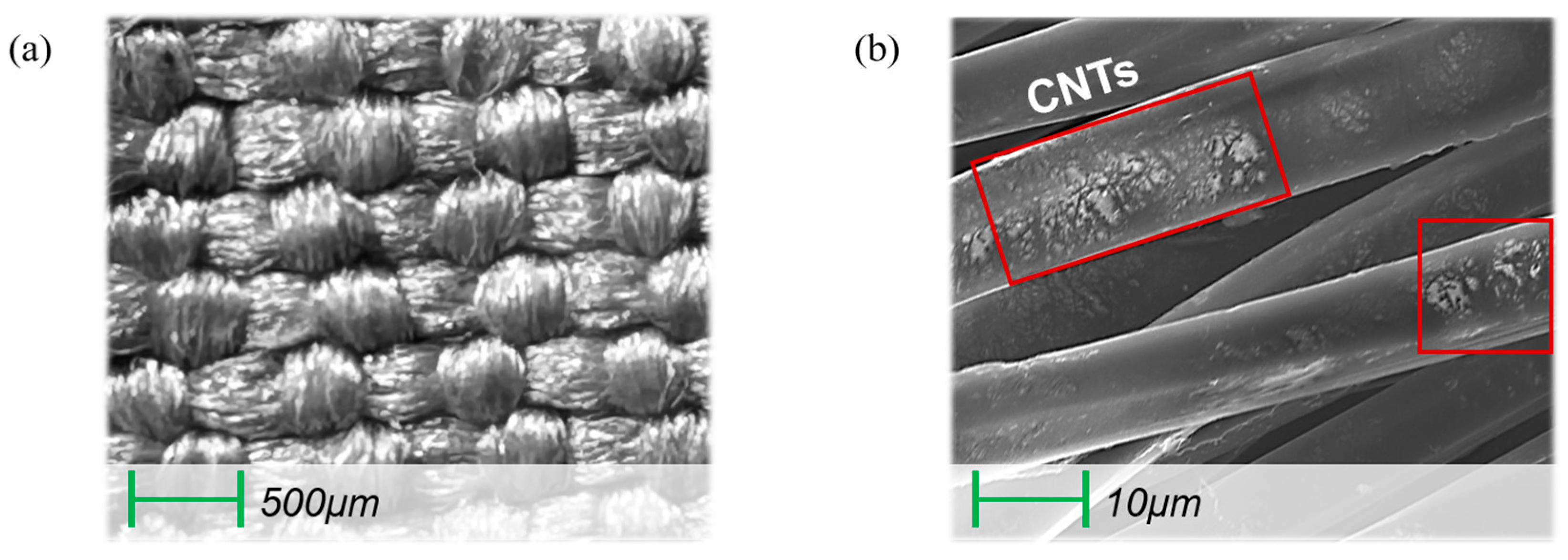
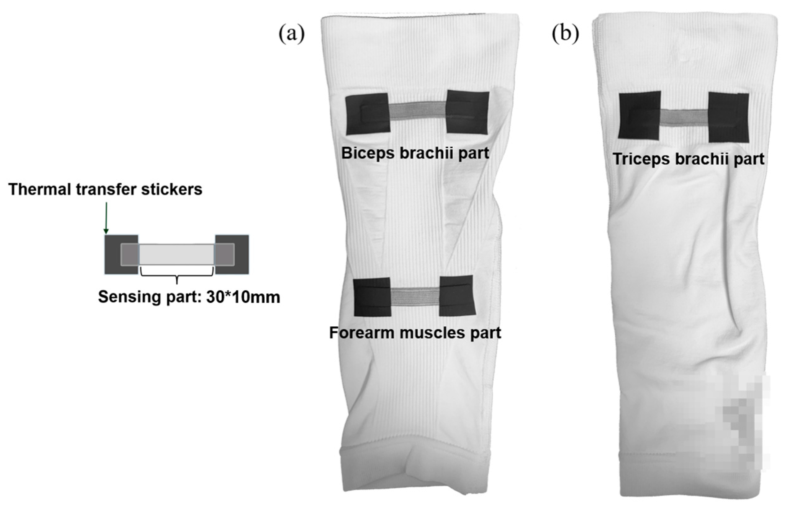
2.1. Fabrication of Textile Stretch Sensors and Application to Arm Sleeve

The E-band (KOLON Co., Ltd., Seoul, Republic of Korea), used as the base material for the textile stretch sensor, is composed of 80% PET and 20% elastane and is woven into a ring shape to provide excellent elasticity and resilience. To impart conductivity to this non-conductive fiber, the E-band was dip-coated with a single-walled carbon nanotube (SWCNT) ink (0.1 wt%). SWCNT, a cylindrical carbon nanostructure known for its exceptional electrical conductivity, is widely used in textiles to enhance conductivity [21,22]. The dip-coating process utilized a water-based SWCNT solution (0.1 wt%) that was stirred at 1000 rpm for 3 h using a magnetic stirrer to ensure uniform dispersion and prevent bubble formation. The E-band was then immersed in the SWCNT solution for 1 h. Following this, a padding machine was employed to ensure deep penetration of the CNT particles into the knit structure. The residual moisture was subsequently removed using a two-way drying machine, which dried the material at 100 °C for 5 min with a circulating fan speed of 1500 rpm. Figure 1 illustrates the dip-coating process used to fabricate the textile stretch sensor.

Three textile stretch sensors were fabricated to measure muscle stretch during the biceps barbell curl exercise, specifically targeting the biceps brachii, triceps brachii, and forearm muscles. Figure 2 illustrates a microscopic image of the dip-coated E-band.

The sensors were affixed to the arm sleeve using thermal transfer stickers. To ensure smooth data collection, it is important that the arm sleeve’s Young’s modulus is higher than that of the E-band, which serves as the stretch sensor. If the sleeve’s modulus is similar to or lower than that of the E-band, other areas of the sleeve may stretch during exercise, potentially interfering with accurate data collection. Considering these factors, the Adidas ADSL-13023 arm sleeve, composed of 92% polyamide and 8% elastane, was selected. Figure 3 shows the fabricated textile stretch sensor attached to the arm sleeve in the exercise measurement area.

During the biceps barbell curl, the distance between CNT particles within the textile stretch sensor dynamically changes, alternately moving closer together or farther apart. This fluctuation causes the sensor’s resistance to increase when tensile force is applied and to return to its initial value during the relaxation phase. The three textile stretch sensors affixed to the arm sleeve experience varying degrees of stretch depending on their attachment points, resulting in distinct resistance changes. Figure 4 illustrates the movement-induced response of the textile stretch sensors when integrated into the arm sleeve.

The biceps barbell curl exercise was conducted at a pace set by a metronome at 50 beats per minute, repeated five times over a duration of 12 s. Resistance data from the textile stretch sensor were acquired using the Arduino Mega 2560 Rev3 (Arduino.cc, Monza, Italy) at a sampling frequency of 370 Hz. Measurements were recorded simultaneously from both ends of the sensing portion, utilizing three channels to capture data from the three sensor attachment points. A fixed resistor of 10 kΩ was employed based on the voltage division principle to ensure accurate resistance measurements.

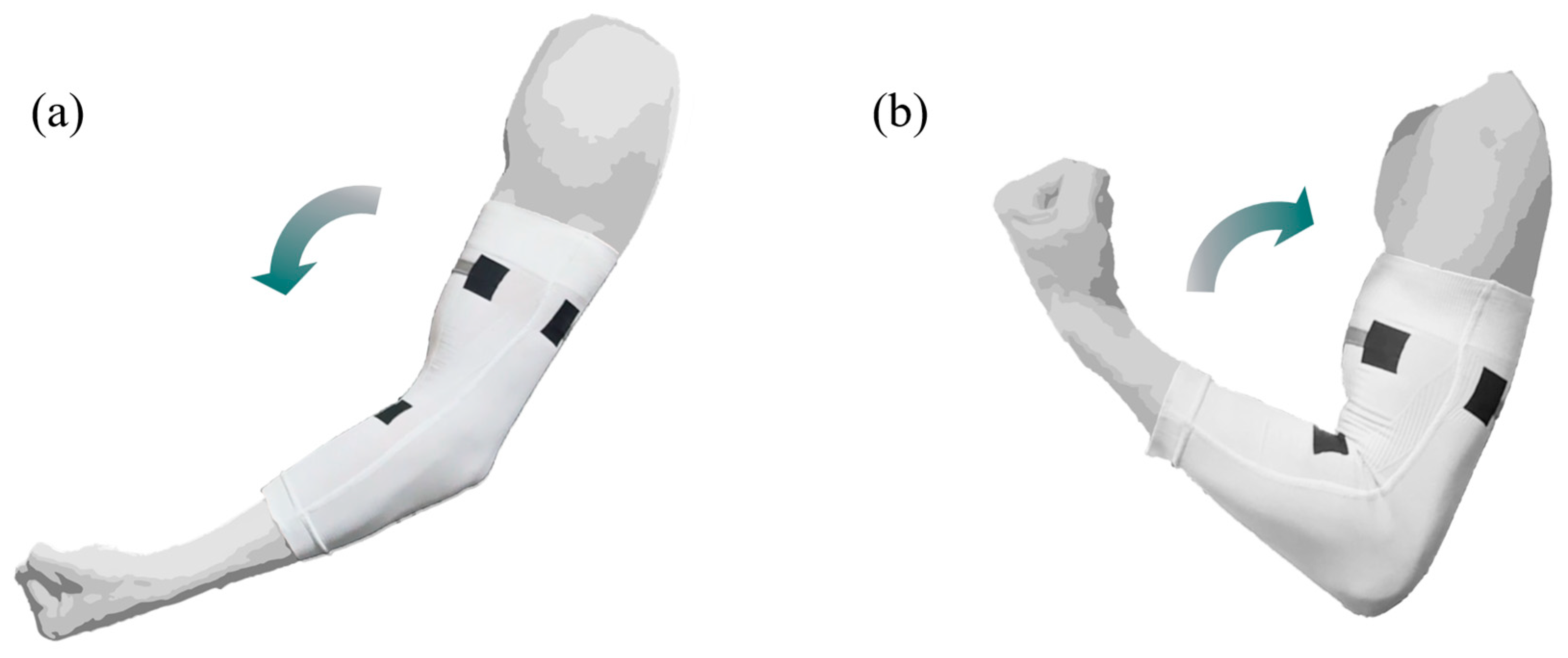
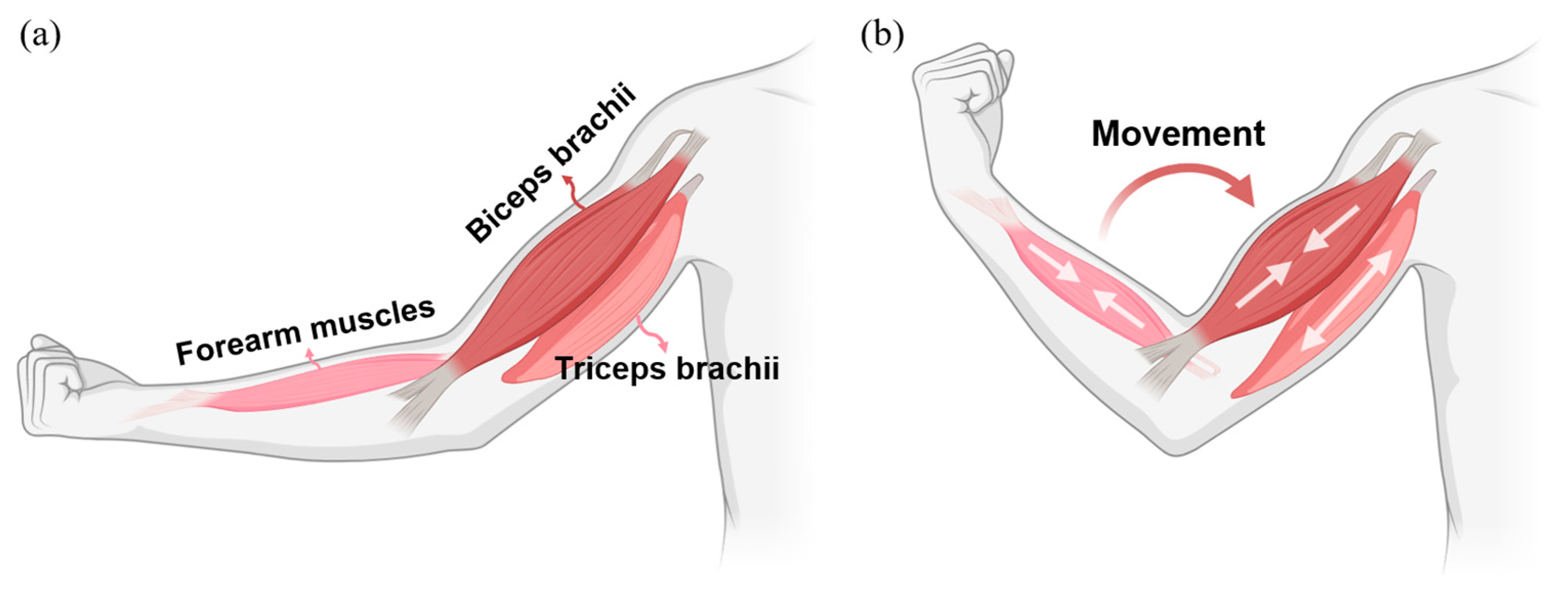
2.2. sEMG Data Collection

sEMG measures the electrical signals generated by muscle fibers through electrodes attached to the skin’s surface, providing a record of muscle activity. As the number of activated muscle fibers increases, both the amplitude of the measured signal and the force generated by the muscle rise correspondingly. However, raw sEMG data often oscillate around the y = 0 line, which can lead to zero-sum issues in calculations such as mean and standard deviation. To address this, sEMG signals are commonly normalized using the root mean square (RMS) method before further analysis (Equation (1)). In Equation (1), $N$ represents the number of samples, and $x_i$ denotes the data values.

$$RMS=\sqrt{{\displaystyle \frac{1}{N}}\sum _{i=1}^N{x}_i^2}$$

(1)

The biceps barbell curl exercise primarily targets the biceps brachii while also engaging the forearm muscles (including the brachioradialis and flexor carpi radialis) and the triceps brachii (Figure 5a). When lifting the barbell, the muscle fibers of the biceps brachii and forearm muscles contract, while those of the triceps brachii relax [23] (Figure 5b).

sEMG sensors (Delsys, Inc., Natick, MA, USA) were attached to the three muscles identified in Figure 5a. To minimize the influence of skin conditions during measurement, hair was removed from each attachment site, and residual skin oils were cleansed with alcohol pads. The biceps barbell curl exercise was performed at a metronome pace of 50 beats per minute, repeated five times over a duration of 12 s. Voltage data collected from the sEMG sensors were normalized to RMS values using EMGworks^® Software (Version 4.8.0), Delsys, Inc., Natick, MA, USA). The sampling frequency was set to 1111 Hz with 16-bit resolution, and the RMS window length was fixed at 0.25 s. To ensure consistency with the textile stretch sensor data in terms of time series and data size, the normalized sEMG data were subsequently downsampled to 370 Hz using MATLAB 2023a (MathWorks Inc., Natick, MA, USA).

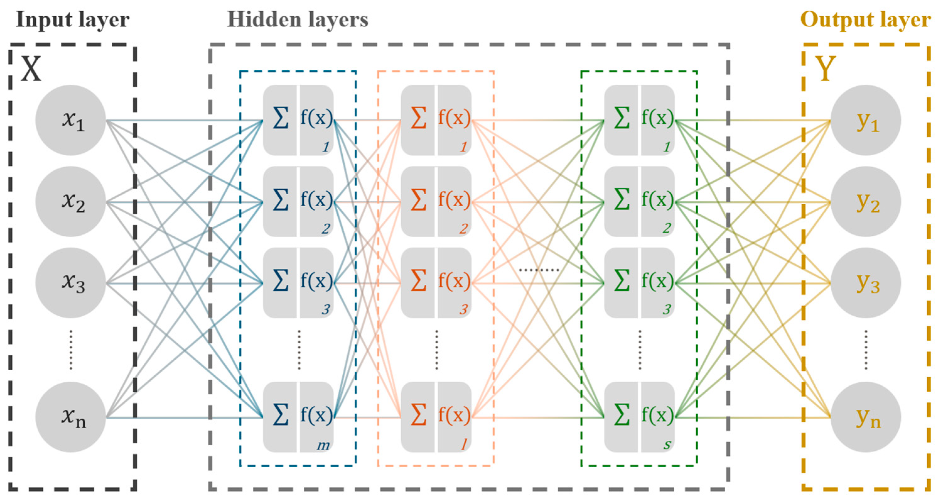
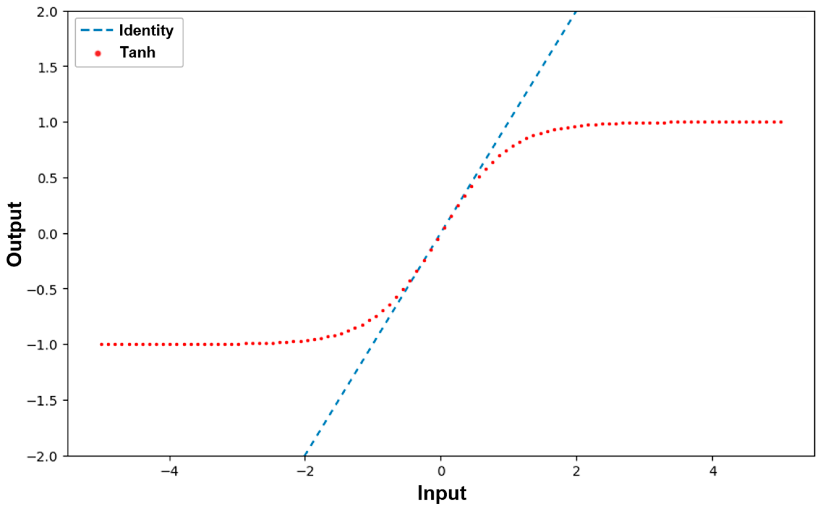
2.3. MLP Learning Process with Causal Relationship Data

The artificial neural network (ANN), which forms the core structure of the MLP, functions as a tool for approximating mathematical relationships. It operates by utilizing matrices composed of real-valued vectors as input and output layers [24]. Within the network, nodes process the input vector values using weights, biases, and activation functions, forwarding the computed values to subsequent layers. Upon reaching the output layer, backpropagation optimizes the weights and biases to minimize the error between actual and predicted values. A schematic representation of the MLP is shown in Figure 6, where the sigma value within each hidden layer node represents the computations involving bias and weights, and f(x) denotes the activation function. The input layer matrix X and output layer matrix Y are composed of vectors x and y, respectively.

In this study, the backpropagation algorithm was utilized, with Mean Squared Error (MSE) serving as the loss function to quantify the difference between the actual and predicted output values. To minimize the loss function, the Levenberg–Marquardt algorithm was employed due to its efficiency in handling nonlinear optimization problems [25]. The formula for MSE is presented in Equation (2). $N$ represents the number of samples, $y_i$ denotes observed values, and ${\widehat{y}}_i$ represents predicted values.

$$MSE={\displaystyle \frac{1}{N}}\sum _{i=1}^N{\left(y_i-{\widehat{y}}_i\right)}^2$$

(2)

Equation (3) presents the formula for the Levenberg-Marquardt algorithm. In this equation, $x_{k+1}$ represents the updated parameter vector at iteration $k+1$, while $x_k$ denotes the parameter vector at iteration $k$, The Jacobian matrix is represented by J, $F$ denotes the difference between observed and predicted values, μ is the damping parameter, and I represents the identity matrix.

$$x_{k+1}=x_k-{\left(J^{T}J+\mu I\right)}^{-1}{J}^{T}F$$

(3)

To ensure sufficient training, the hyperparameters were configured as follows: epoch = 1000, learning rate = 0.01, minimum gradient of the loss function = 1 × 10⁻⁴⁰, and momentum constant = 1 × 10⁻⁴⁰. The dataset was divided into training, validation, and test sets in a ratio of 70:15:15.

In deep learning algorithms, varying activation functions across hidden layers can sometimes improve model accuracy. However, to minimize the influence of activation function differences on model performance, this study uniformly applied the Hyperbolic Tangent (Tanh) function to all four hidden layers (Equation (4)). The Tanh function, commonly used in deep learning, restricts the output range between −1 and 1 while maintaining symmetry around 0, which helps stabilize the learning process in complex neural networks.

$$Tanh x={\displaystyle \frac{\mathit{sinh}x}{\mathit{cosh}x}}={\displaystyle \frac{e^x-e^{-x}}{e^x+e^{-x}}}$$

(4)

The network architecture included 10 nodes in each hidden layer. Given the model’s purpose of predicting continuous values, the identity function was applied in the output layer to produce output values identical to the input values. The model architecture, including the number of hidden layers, nodes per layer, and activation functions, was not predetermined by theoretical derivations but was empirically optimized based on prior research and experimental validation [26,27]. These parameters were selected to align with the dataset characteristics while ensuring model stability and generalization. Figure 7 illustrates the graphs of the activation functions utilized in the network. All algorithms and computations were implemented using MATLAB.

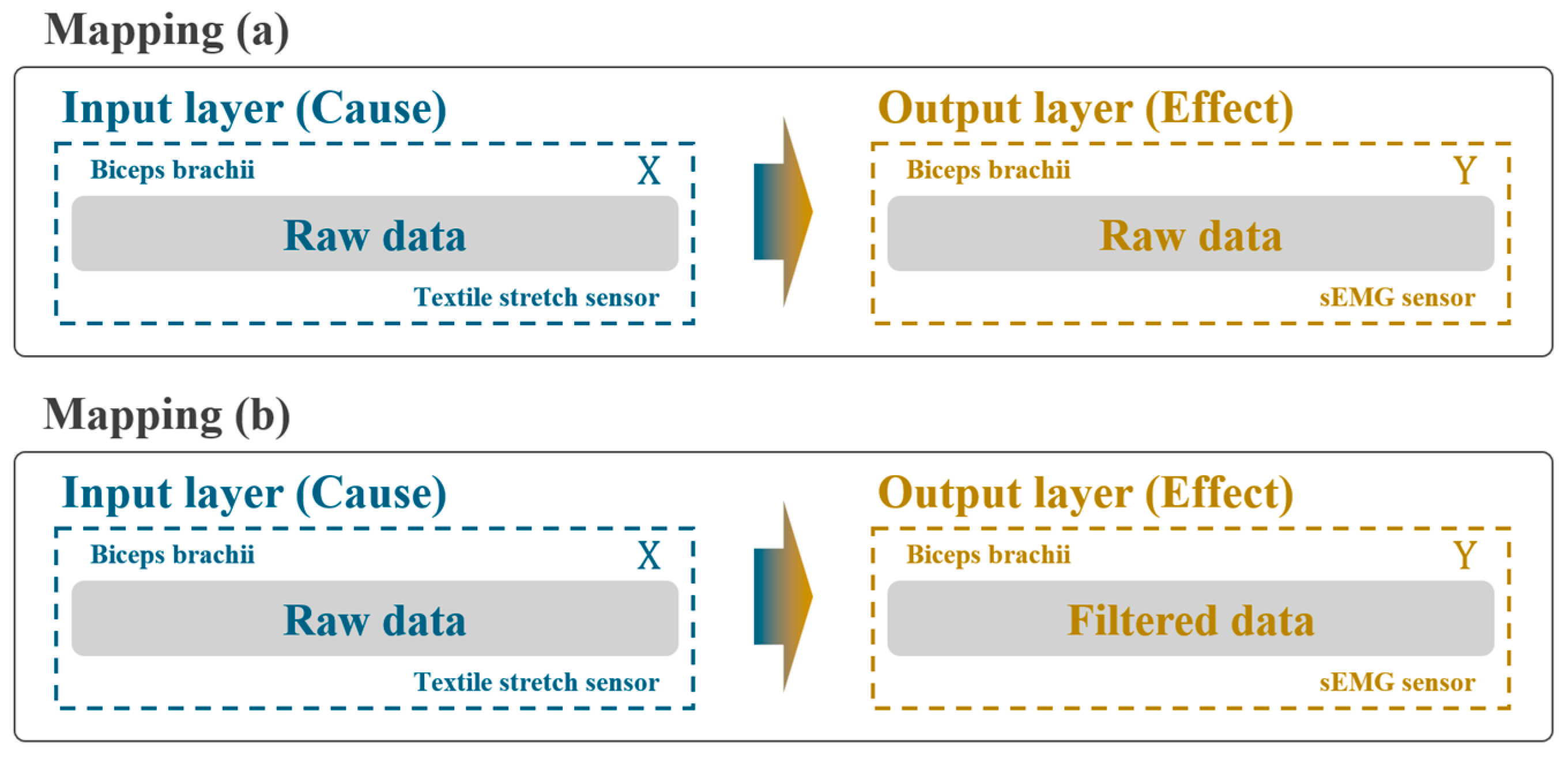
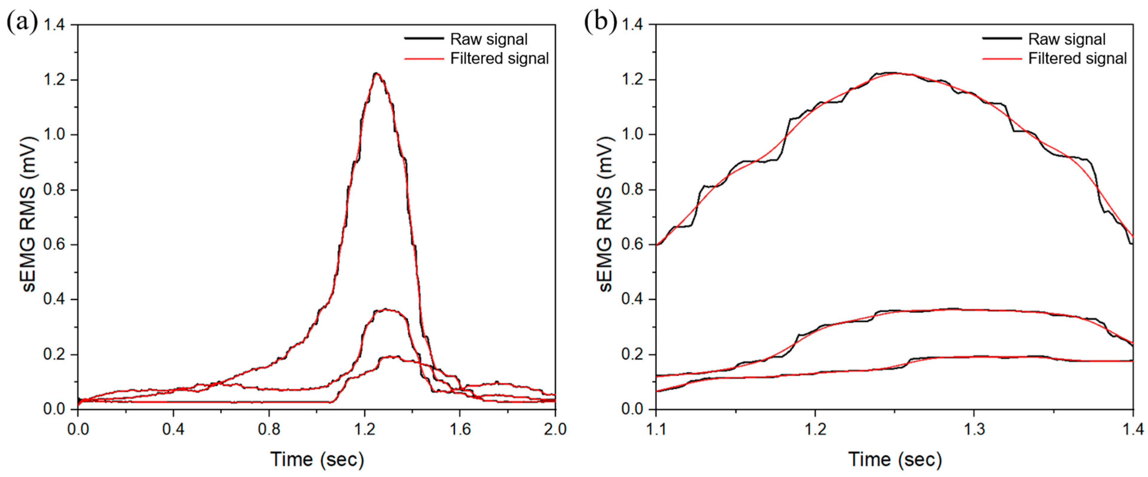
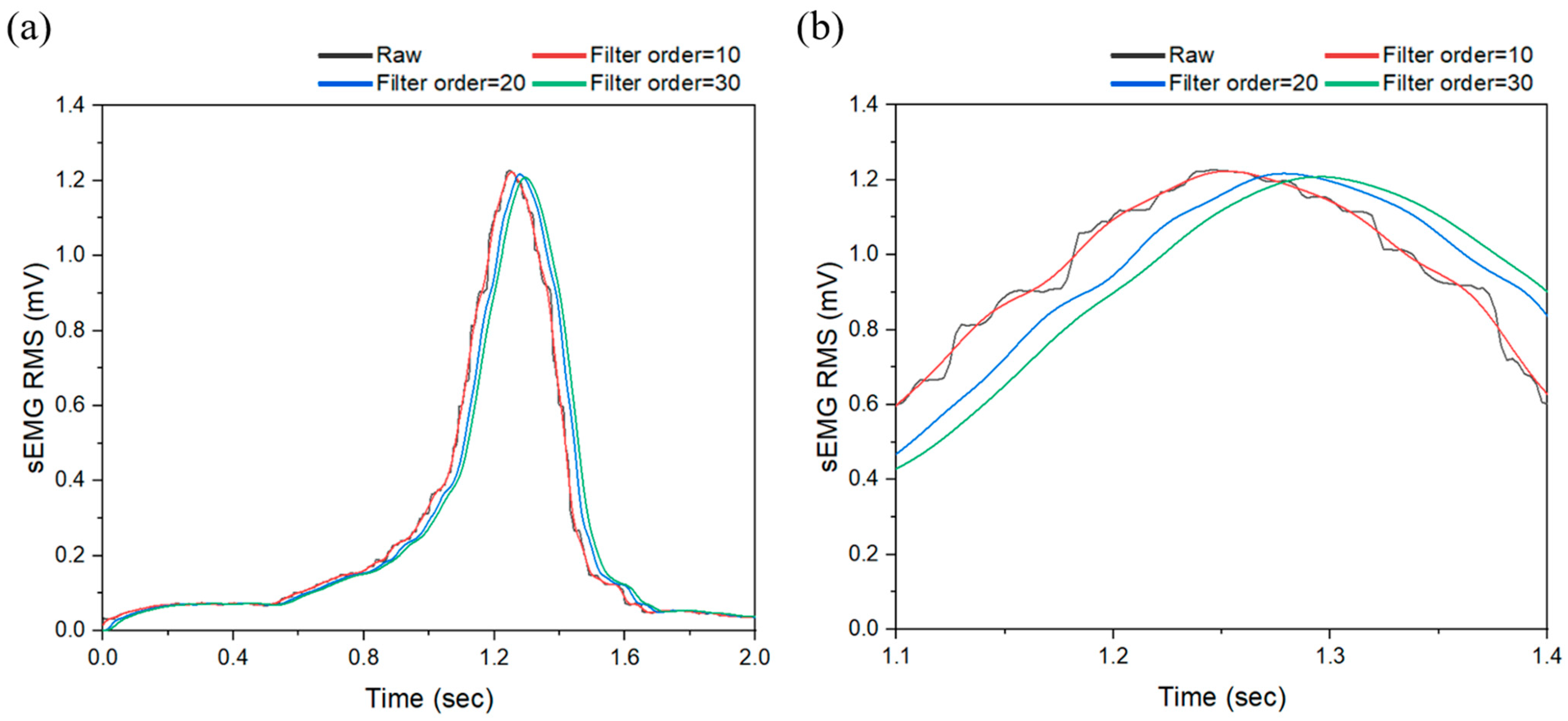
2.3.1. First Stage: Effect of Low-Pass FIR Filter

The first stage evaluates the accuracy of the trained model by comparing the results with and without the application of a low-pass FIR filter during the mapping of textile stretch sensor data to the sEMG data collected from the biceps brachii.

The low-pass FIR filter is a type of finite impulse response filter that allows low-frequency signals to pass while attenuating high frequencies, enabling the removal of noise and the enhancement of meaningful signal features [28]. By highlighting the underlying trends and key characteristics of the data, this filtering process is expected to improve the accuracy of machine learning models [29].

For this study, the cutoff frequency of the low-pass FIR filter was set to 3 Hz. Given that the biceps barbell curl exercise was performed at a frequency of 0.417 Hz in synchronization with the metronome, signals above 3 Hz were classified as noise, except for potential measurement errors [30]. This implementation was carried out using MATLAB’s built-in algorithm, and the formula for the low-pass FIR filter is presented in Equation (5). y(n) represents the output signal, x(n) represents the input signal, $b_k$ denotes the FIR filter coefficients, and N − 1 signifies the value obtained by subtracting the delay from the length of the FIR filter.

$$y\left(n\right)={\sum }_{k=0}^{N-1}{b}_{k}x(n-k)$$

(5)

Figure 8 illustrates the schematic diagram for Stage 1. In Mapping (a), raw sEMG signals were directly mapped, whereas in Mapping (b), sEMG signals were preprocessed using a low-pass FIR filter before mapping. The sEMG data utilized for subsequent mapping stages were selected based on the results of Stage 1, depending on whether raw or filtered data demonstrated better performance.

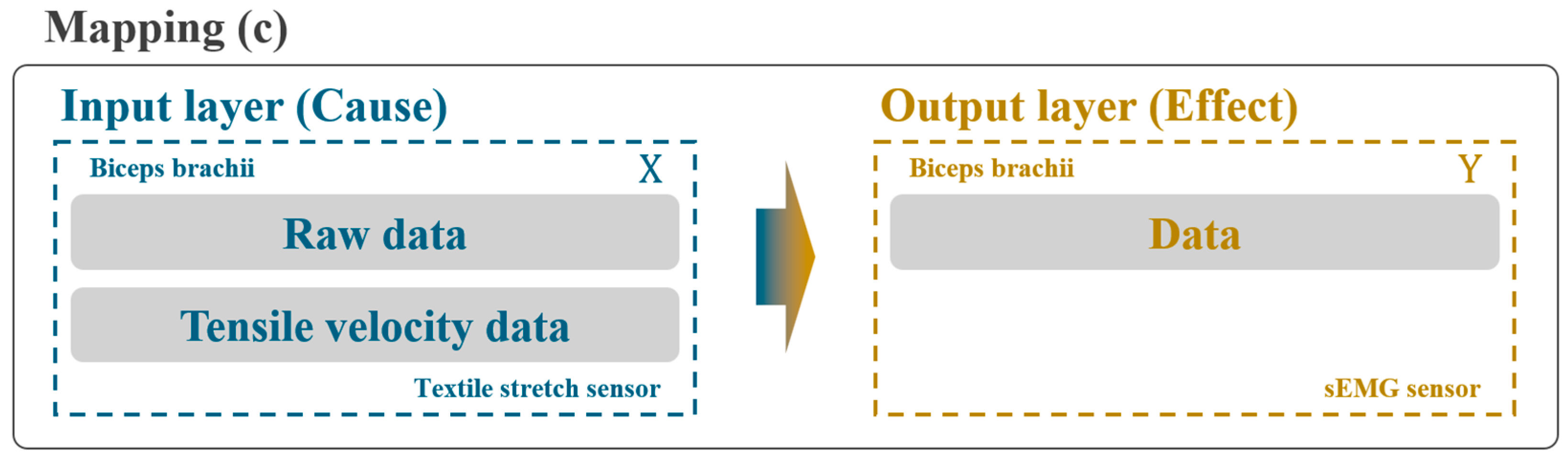
2.3.2. Second Stage: Integration with Tensile Velocity Data

In the second stage, the tensile velocity data of the textile, calculated based on the sampling frequency, were incorporated into the textile stretch sensor data collected from the biceps brachii. By adding tensile velocity data to the input layer matrix corresponding to the cause, the vector $x_n$, which previously formed the matrix X, is expanded into a two-dimensional vector (Figure 6).

The resistance values measured using the textile stretch sensors were normalized using the relative change in resistance, as defined in Equation (6). $R_0$ represents the initial resistance value, and $R_f$ denotes the measured resistance value. In the elastic region of the textile stretch sensor, the strain value is linearly proportional to ${\displaystyle \frac{∆R}{R_0}}$.

$$Relative change in resistance={\displaystyle \frac{R_f-R_0}{R_0}}={\displaystyle \frac{∆R}{R_0}}$$

(6)

A value proportional to the tensile velocity can be derived by dividing ${\displaystyle \frac{∆R}{R_0}}$ by the sampling frequency, as shown in Equation (7).

$$Tensile velocity\propto {\displaystyle \frac{{\left(\frac{∆R}{R_0}\right)}_{k+1}-{\left(\frac{∆R}{R_0}\right)}_k}{Sampling frequency}}$$

(7)

Figure 9 presents the schematic diagram for Stage 2. In Mapping (c), the relationship between matrix X, composed of two-dimensional vectors as nodes, and matrix Y, composed of one-dimensional vectors as nodes, was established. Subsequently, the mapping results were compared with those approaches from Stage 1 that exhibited superior accuracy.

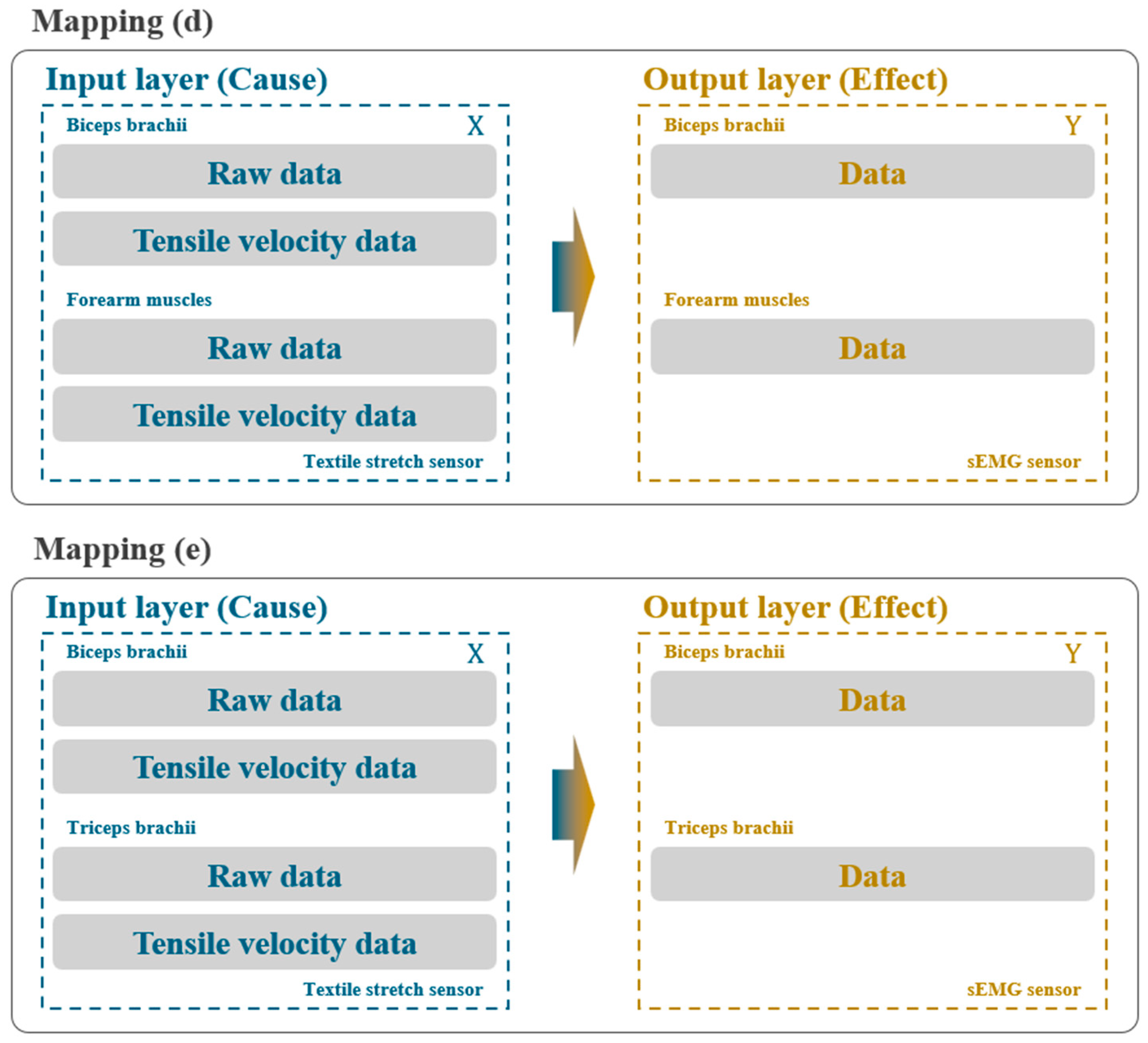
2.3.3. Third Stage: Expanding Dataset for Mapping Accuracy Comparison

In the third stage, additional datasets measured from regions other than the biceps brachii were incorporated into the dataset used in Mapping (c), and new mappings were performed. Figure 10 illustrates the schematic diagrams of mappings (d) and (e). In Mapping (d), data from the textile stretch sensors on the forearm muscles, along with tensile velocity data, were added to the input layer, while sEMG data from the corresponding area were added to the output layer. As a result, the matrix X representing the cause consists of 4-dimensional vectors, while the matrix Y representing the effect consists of 2-dimensional vectors. Similarly, in Mapping (e), data from the triceps brachii were incorporated into both the input and output layers. The accuracy of the trained models from mappings (d) and (e) was then compared to the results obtained in Stage 2.

Finally, mapping was conducted by incorporating the datasets from all measured areas into both the input and output layers. Figure 11 illustrates the schematic diagram for Mapping (f). In this mapping, data from textile stretch sensors on the forearm muscles and triceps brachii, along with tensile velocity data, were added to the input layer, while the corresponding sEMG data were added to the output layer. As a result, the matrix X, representing the cause, consists of 6-dimensional vectors, while the matrix Y, representing the effect, consists of 3-dimensional vectors. Among the mapping methods used in this study, Mapping (f) demonstrates the strongest causal relationship between the datasets.

3. Results

3.1. Textile Stretch Sensor Data Results

To evaluate the mechanical and electrical properties of the textile stretch sensor, the arm sleeve and dip-coated E-band were subjected to 100% elongation from 30 mm to 60 mm at a controlled speed of 1 mm per second using a universal testing machine (UTM). Figure 12a illustrates the strain–stress curves for both the arm sleeve and the dip-coated E-band, highlighting their elastic behavior under applied stress. Additionally, Figure 12b presents the graph showing the relative change in resistance as a function of the elongation of the dip-coated E-band, demonstrating its sensitivity to strain.

For the E-band, the modulus’s R-squared value decreased to 0.95 or below at strain levels of 80% or higher, defining its elastic region up to 80% strain. At this point, Young’s modulus was measured to be 0.2622. In contrast, the arm sleeve maintained an R-squared value of 0.99 even at 100% strain, with a Young’s modulus of 0.4732.

Figure 13 illustrates the variation in tensile data measured through three textile stretch sensors over time. The maximum value of ${\displaystyle \frac{∆R}{R_0}}$ was recorded as 0.853, corresponding to a strain of 12.53% (see Figure 12b).

RMS and standard deviation were employed to quantify the amplitude values of the textile stretch sensor data corresponding to each muscle (Figure 14). The RMS values for the forearm muscles, biceps brachii, and triceps brachii were 0.446, 0.232, and 0.178, respectively. Similarly, the standard deviations were 0.3142 for the forearm muscles, 0.1322 for the biceps brachii, and 0.1053 for the triceps brachii.

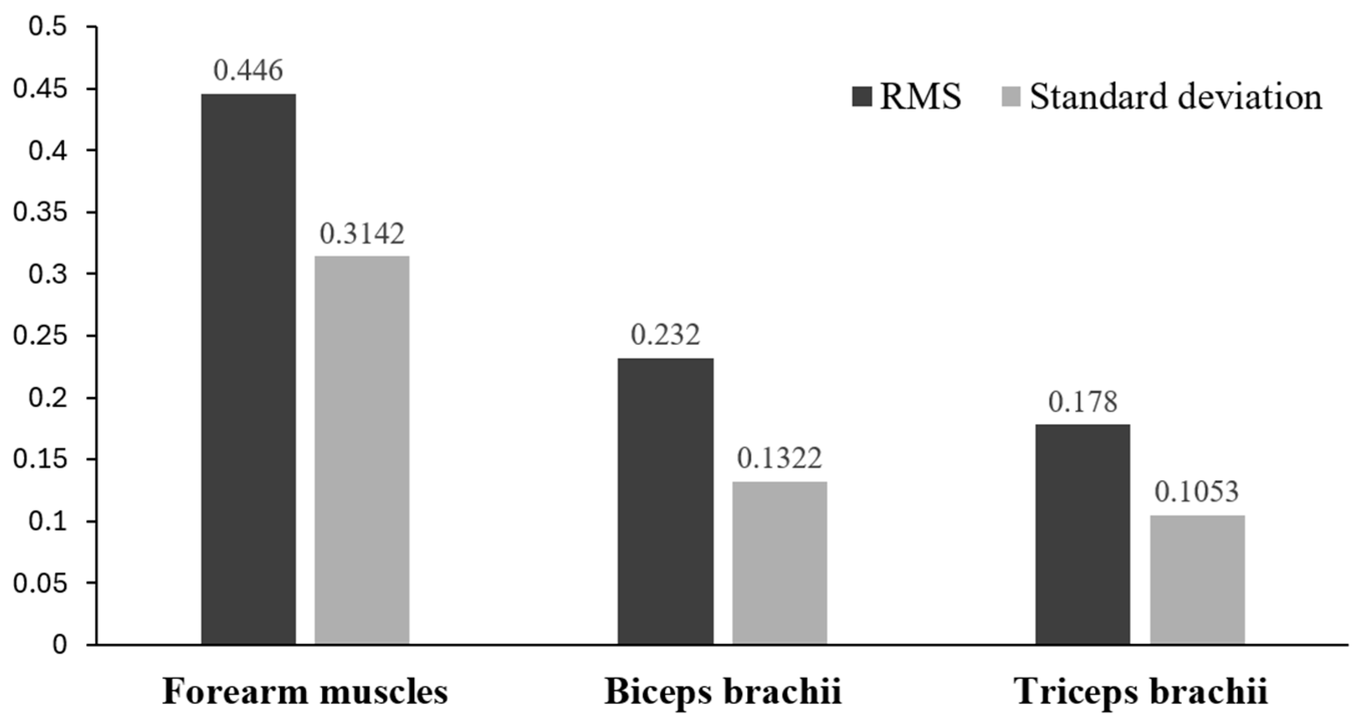
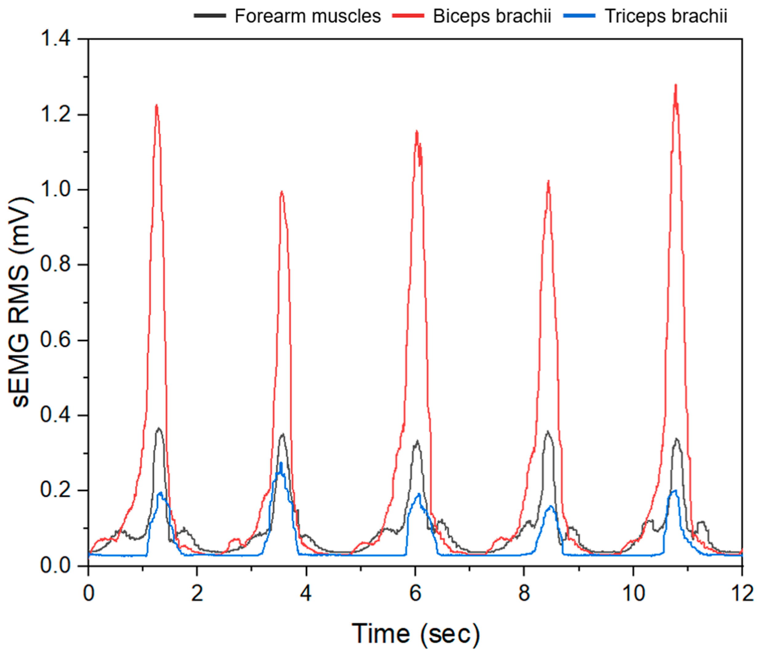
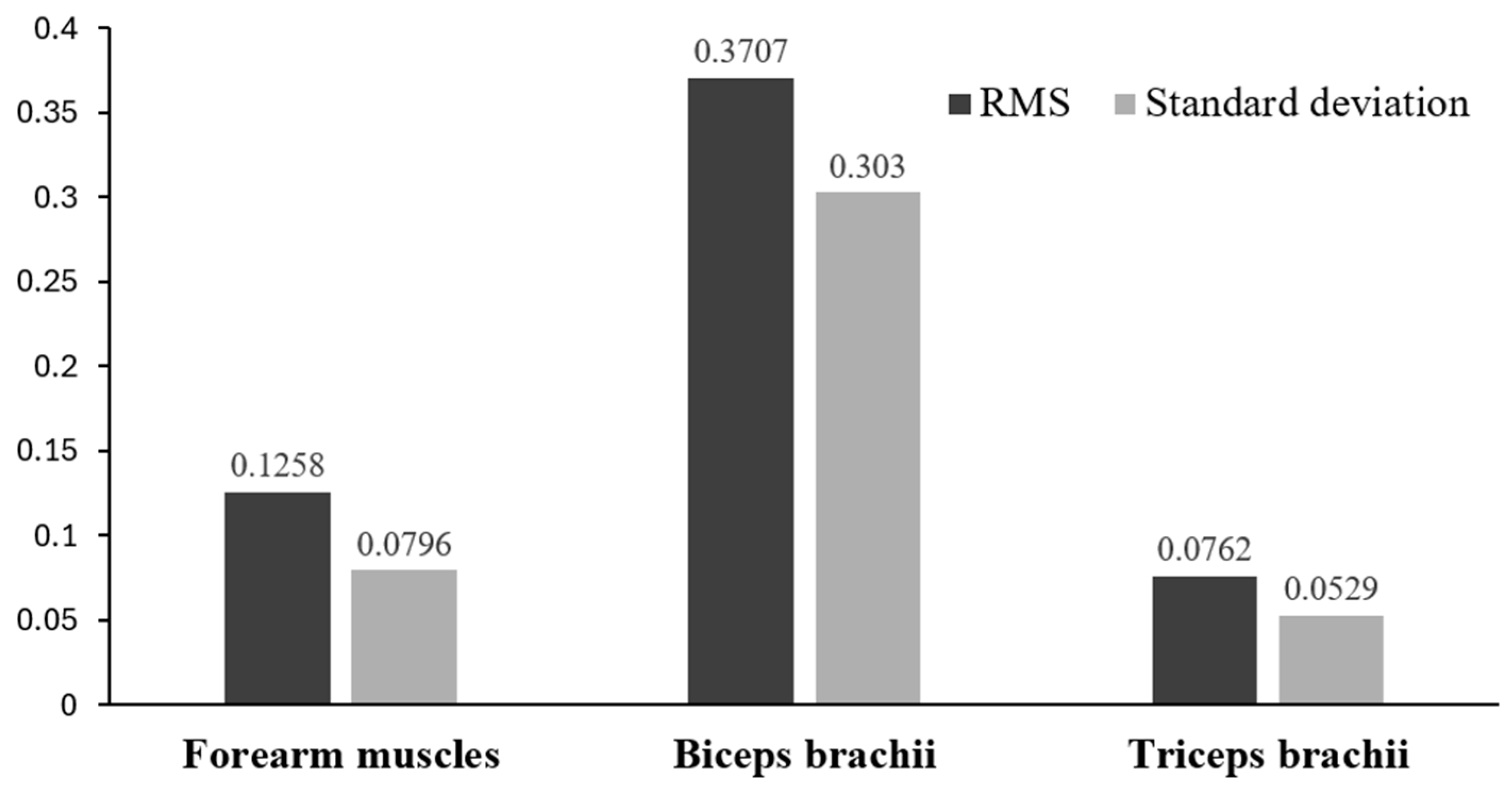
3.2. sEMG Data Results

Figure 15 illustrates the temporal variation of electromyographic signals measured using three sEMG sensors. During the biceps barbell curl exercise, the peak values of the sEMG signals varied, reflecting differences in contraction strength among the muscles.

Figure 16 presents the quantification of sEMG signal amplitude values using RMS and standard deviation. The RMS values for the forearm muscles, biceps brachii, and triceps brachii were 0.1258, 0.3707, and 0.0762, respectively. Similarly, the corresponding standard deviations were 0.0796 for the forearm muscles, 0.3030 for the biceps brachii, and 0.0529 for the triceps brachii.

Figure 17 illustrates the analysis of the collected sEMG data using fast Fourier transform (FFT) and power spectral density (PSD). The highest peak for each muscle was observed at 0.417 Hz, corresponding to the metronome rhythm used during the exercise.

In the FFT analysis of the biceps brachii, the amplitude at the highest peak observed at 0.417 Hz was 0.301. The PSD analysis revealed that the power in the 0.417 Hz band was 0.5254 dB/Hz, which is approximately 3.82 times greater than the average power across the frequency band. The results of the FFT and PSD analyses for the forearm muscles, biceps brachii, and triceps brachii are summarized in

Table 1. FFT and PSD analysis of measured muscles.

Muscle	Peak Frequency (Hz)	Peak Amplitude (Arb. Units)	PSD at Peak (dB/Hz)	Total PSD (dB/Hz)
Forearm muscles	0.417	0.082	0.0411	0.0158
Biceps brachii	0.417	0.301	0.5254	0.1374
Triceps brachii	0.417	0.047	0.0134	0.0058

.

Figure 18 presents comparison graphs of sEMG data with and without the application of a low-pass FIR filter with a cutoff frequency of 3 Hz. A magnified section of the time series is included to visually highlight the differences in signal characteristics before and after the filter application.

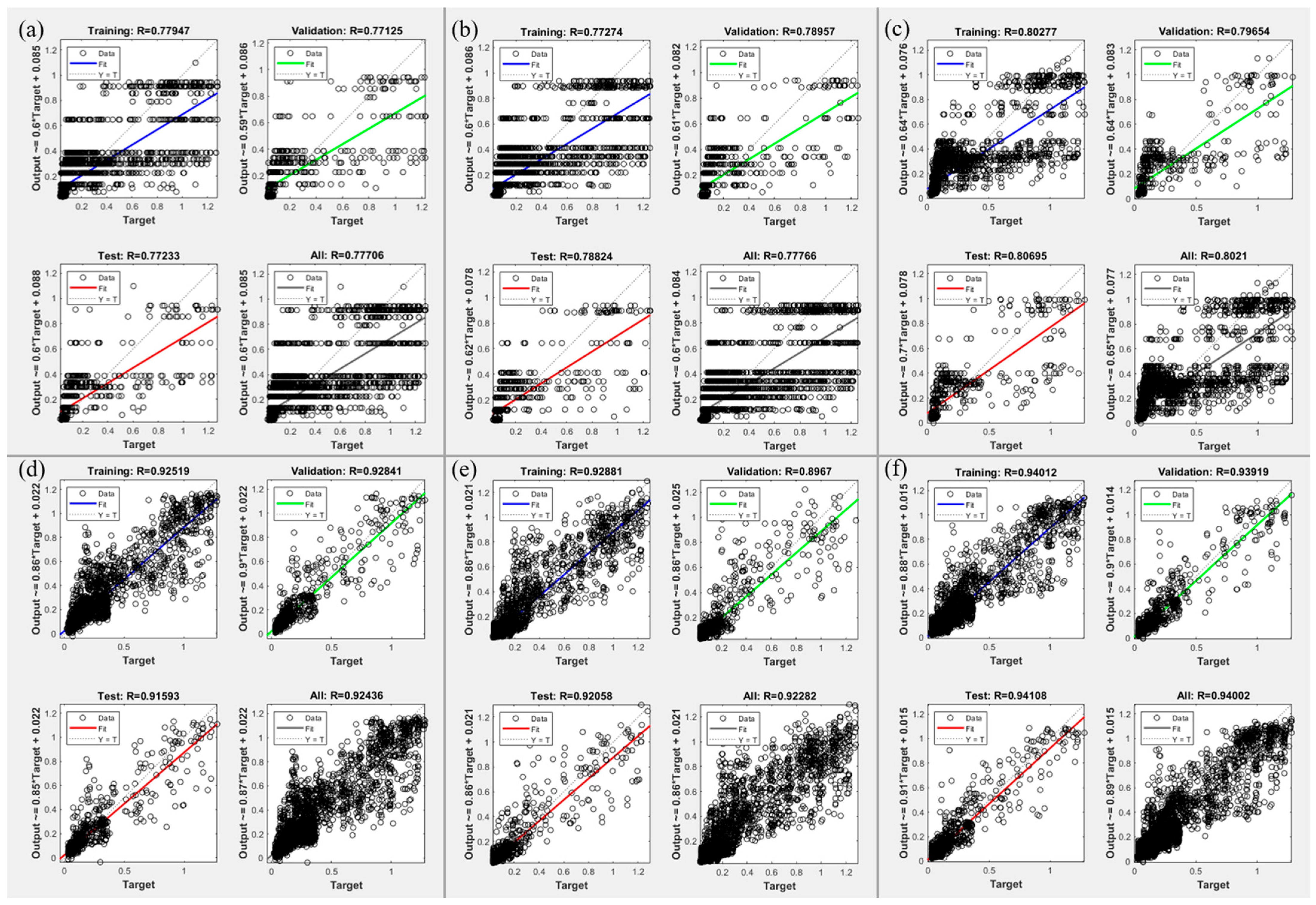
3.3. MLP: Mapping Accuracy Results

3.3.1. Result of First Stage: Low-Pass FIR Filter Application

The R-squared value obtained through mapping serves as a statistical indicator of the model’s fitness, representing the proportion of variability in the dependent variable explained by the model. This value ranges between 0 and 1, with higher values indicating a better model fit to the data.

In Mapping (a), direct mapping was performed between the biceps brachii’s textile stretch sensor data and sEMG raw data. The R-squared values of the MLP regression model were 0.77947 for the training dataset, 0.77125 for the validation dataset, and 0.77233 for the test dataset. Conversely, in Mapping (b), a low-pass FIR filter was applied to the sEMG data prior to mapping. The corresponding R-squared values were 0.77274 for the training dataset, 0.78957 for the validation dataset, and 0.78824 for the test dataset.

Although Mapping (b) employed a low-pass FIR filter to reduce noise in the data, the difference in R-squared values compared to Mapping (a) was minimal. To further investigate the impact of the cutoff frequency, additional mappings were performed using a cutoff frequency lower than the original 3 Hz. The results of these mappings, along with those of Mapping (a), are presented in

Table 2. Mapping results of textile stretch sensor and sEMG data according to cutoff frequency differences.

Mapping	Cutoff Frequency (Hz)	Training ($R^2$)	Validation ($R^2$)	Test ($R^2$)
a	-	0.77947	0.77125	0.77233
b	3	0.77274	0.78957	0.78824
	2.5	0.76703	0.75108	0.74565
	2	0.76198	0.74913	0.77064
	1.5	0.76829	0.73518	0.74350
	1.0	0.76244	0.75156	0.76698
	0.5	0.75180	0.75726	0.79812
	0.1	0.76282	0.79705	0.72023

.

The FFT analysis revealed that even when the peak at 0.417 Hz (Figure 17b), representing the highest peak, passed through a stop band exceeding 0.1 Hz, the difference in mapping results remained negligible. As a result, the filter order of the cutoff frequency was adjusted to investigate its impact. Figure 19 illustrates the comparison graphs between the raw signal and the results when the filter order, initially set to 10, was modified to 20 and 30, respectively, while maintaining the cutoff frequency at 3 Hz.

As the filter order increased, a group delay phenomenon was observed, causing the graph to shift to the right, as shown in Figure 19. The FIR filter applies a window function to the input signal during filtering, and an increase in filter order results in an extended window length. This extension leads to group delay as the input signal propagates to the output. Figure 19b illustrates the results when a filter order of 10 was applied.

Based on the Stage 1 experiment results, the mapping patterns appeared consistent regardless of whether the low-pass FIR filter was applied to the RMS-processed sEMG signals. Therefore, for subsequent stages, raw sEMG data were used for training.

3.3.2. Result of Second Stage: Effect of Tensile Velocity Data

In Mapping (c), the input layer was expanded into a two-dimensional vector by incorporating tensile velocity data of the textile with the textile stretch sensor data from the biceps brachii. The R-squared values of the MLP regression model were 0.80277 for the training dataset, 0.79654 for the validation dataset, and 0.80695 for the test dataset, representing increases of 0.02330, 0.02529, and 0.03462, respectively, compared to the results of Mapping (a).

The experiments in Stage 2 confirmed that adding tensile velocity data to the cause dataset in the input layer improved the overall accuracy of the model. The learning curve for Mapping (c), as shown in Figure 20, illustrates rapid convergence during the initial training epochs, followed by gradual stabilization across the training, validation, and test datasets. The R-squared values for the training dataset reached a stable state at approximately 50 epochs, with similar trends observed for the validation and test datasets.

3.3.3. Result of Third Stage: Effect of Multi-Muscle Data Integration

In Mapping (d), textile stretch sensor data and tensile velocity data from the forearm muscles were added to the input layer, alongside the data from the biceps brachii. The corresponding sEMG data from the forearm muscles were added to the output layer for mapping. The R-squared values of the MLP regression model were 0.92519 for the training dataset, 0.92841 for the validation dataset, and 0.91593 for the test dataset, representing increases of 0.12242, 0.13187, and 0.10898, respectively, compared to Mapping (c).

Similarly, in Mapping (e), the dataset of the triceps brachii was added for mapping. The R-squared values of the MLP regression model were 0.92881 for the training dataset, 0.89670 for the validation dataset, and 0.92058 for the test dataset. Compared to Mapping (c), these values increased by 0.12604, 0.10016, and 0.11363, respectively. However, compared to Mapping (d), the R-squared values showed increases of 0.00362 and 0.00465 for the training and test datasets, respectively, while the validation dataset exhibited a decrease of 0.03171.

Lastly, in Mapping (f), the data from all measured areas were integrated for mapping. The R-squared values were 0.94012 for the training dataset, 0.93919 for the validation dataset, and 0.94108 for the test dataset, making it the model with the highest accuracy among the approaches tested. The results of Mappings (c) to (f) are summarized in

Table 3. Comparison of R-squared values for different mapping approaches: (c) to (f).

Mapping	Training ($R^2$)	Validation ($R^2$)	Test ( $R^2$)
(c)	0.80277	0.79654	0.80695
(d)	0.92519	0.92841	0.91593
(e)	0.92881	0.89670	0.92058
(f)	0.94012	0.93919	0.94108

.

Figure 21 presents the regression analysis results of the models utilizing MLP. Among the mappings, Mapping (f), which integrated data from all muscle groups, achieved the highest R-squared value of approximately 0.94.

4. Discussion

The results of this study indicate that mapping muscle activity using textile stretch sensors and a basic deep learning model, MLP, is a feasible approach. Although MLP is a relatively simple model, it demonstrated a meaningful level of accuracy in predicting sEMG signals. As shown in Table 3, the highest R² value (~0.94) was achieved in Mapping (f), where data from multiple muscle groups—including the biceps brachii, forearm muscles, and triceps brachii—were collectively used. This suggests that expanding the dataset to include additional muscle groups meaningfully enhances predictive performance. Such an outcome is consistent with previous work, emphasizing that comprehensive datasets contribute to improved physiological signal estimation [31].

One key observation from the experimental results is that applying a low-pass FIR filter to the sEMG signals (Stage 1) had minimal impact on prediction accuracy. Table 2 presents a comparison of R² values obtained with different cutoff frequencies. When a 3 Hz FIR filter was applied, the R² values changed only slightly from 0.779 (raw data) to 0.773 for the test dataset, showing a negligible difference. Even when the cutoff frequency was further adjusted to 2 Hz or 1.5 Hz, no significant improvement was observed. This suggests that in this particular context, root mean square (RMS) preprocessing alone was sufficient to suppress noise, likely due to the already downsampled nature of the sEMG data.

Additionally, incorporating tensile velocity data from the textile stretch sensor (Stage 2) improved the mapping accuracy. As seen in Table 3, the R² value increased from 0.77233 (Mapping (a), without tensile velocity) to 0.80695 (Mapping (c), with tensile velocity), demonstrating a relative improvement of approximately 4.5%. This finding suggests that the dynamic aspects of muscle movement, which are not fully captured by strain-based measurements alone, provide valuable complementary information for mapping. Since tensile velocity is derived from the sampling rate of the stretch sensor, it does not require additional measurement devices, making it a practical and efficient feature for wearable sensor applications.

The most significant improvement in predictive performance was observed when data from multiple muscle groups were integrated (Stage 3). Figure 21 illustrates the regression analysis results for different mappings. When only biceps brachii data were used (Mapping (c)), the test dataset R² value was 0.80695. However, adding forearm muscle data (Mapping (d)) significantly increased the test dataset R² to 0.91593, and incorporating triceps brachii data (Mapping (e)) further improved it to 0.92058. Ultimately, when data from all three muscle groups were included (Mapping (f)), the highest test R² value of 0.94108 was achieved. This result underscores the role of muscle synergy, where multiple muscles contribute to movement even if a particular muscle is the primary target of an exercise [32,33].

While the inclusion of triceps brachii data improved overall accuracy, its contribution was relatively smaller than that of the forearm muscles. This is likely due to the antagonistic nature of the triceps brachii during biceps barbell curls, resulting in a weaker correlation with biceps brachii activity. Nevertheless, the addition of supporting muscle group data enhanced the overall robustness of the model, demonstrating that incorporating data from biomechanically relevant muscles strengthens predictive models in physiological signal estimation.

5. Conclusions

This study investigated the feasibility of mapping muscle activity using textile stretch sensors and a basic MLP model. A three-stage experimental approach was employed to assess the impact of preprocessing techniques, additional input variables, and multi-muscle data integration on mapping accuracy.

The results demonstrated that applying a low-pass FIR filter to sEMG signals had a minimal effect on model performance, suggesting that RMS preprocessing was sufficient for noise reduction in this context. Furthermore, incorporating tensile velocity data as an additional input feature improved prediction accuracy, highlighting the potential benefit of integrating dynamic muscle movement characteristics. The highest accuracy was achieved when data from multiple muscle groups were included, indicating that expanding the dataset beyond a single muscle region enhances mapping performance.

While these findings provide insight into the potential of textile stretch sensors for estimating muscle activity, several limitations remain. First, the experiment focused on a single type of exercise, and it remains unclear whether similar mapping performance can be achieved for other movements. Given that different exercises involve varying muscle activation patterns, additional studies are needed to validate the generalizability of the proposed approach. Second, the dataset was obtained from a limited number of participants, which may affect the robustness of the model. Future research should consider expanding the dataset to include a more diverse population to improve the reliability of the findings. Third, while this study employed MLP as a baseline deep learning model, more advanced architectures, such as convolutional neural networks (CNNs) or recurrent neural networks (RNNs), may further enhance prediction accuracy. Investigating the effectiveness of these models in textile stretch stretch-sensor-based muscle activity mapping would be a meaningful direction for future work.

Despite these limitations, this study contributes to the growing body of research on wearable sensor-based muscle activity monitoring. The results suggest that textile stretch sensors, when combined with appropriate machine learning models, could be a practical alternative for estimating muscle activity in various applications, including sports science and rehabilitation. Future studies should aim to refine model architectures, expand experimental conditions, and explore additional physiological parameters to further enhance the utility of textile-based wearable sensing technologies.

References

1. Luczak, T.; Saucier, D.; Burch, V.R.F.; Ball, J.E.; Chander, H.; Knight, A.; Wei, P.; Iftekhar, T. Closing the wearable gap: Mobile systems for kinematic signal monitoring of the foot and ankle. Electronics 2018, 7, 117. [Google Scholar] [CrossRef]
2. Mukhopadhyay, S.C. Wearable sensors for human activity monitoring: A review. IEEE Sens. J. 2014, 15, 1321–1330. [Google Scholar]
3. Korhonen, I.; Parkka, J.; Van Gils, M. Health monitoring in the home of the future. IEEE Eng. Med. Biol. Mag. 2003, 22, 66–73. [Google Scholar]
4. Trung, T.Q.; Lee, N.E. Flexible and stretchable physical sensor integrated platforms for wearable human-activity monitoringand personal healthcare. Adv. Mater. 2016, 28, 4338–4372. [Google Scholar] [PubMed]
5. Yao, S.; Swetha, P.; Zhu, Y. Nanomaterial-enabled wearable sensors for healthcare. Adv. Healthc. Mater. 2018, 7, 1700889. [Google Scholar]
6. Wang, M.; Wang, T.; Luo, Y.; He, K.; Pan, L.; Li, Z.; Cui, Z.; Liu, Z.; Tu, J.; Chen, X. Fusing stretchable sensing technology with machine learning for human–machine interfaces. Adv. Funct. Mater. 2021, 31, 2008807. [Google Scholar]
7. Kwon, S.H.; Dong, L. Flexible sensors and machine learning for heart monitoring. Nano Energy 2022, 102, 107632. [Google Scholar]
8. Liao, X.; Song, W.; Zhang, X.; Huang, H.; Wang, Y.; Zheng, Y. Directly printed wearable electronic sensing textiles towards human–machine interfaces. J. Mater. Chem. C 2018, 6, 12841–12848. [Google Scholar]
9. Chun, S.; Kim, J. Textile smart sensors based on a biomechanical and multi-layer perceptron hybrid method. J. Ind. Text. 2023, 53, 15280837231208226. [Google Scholar]
10. Shen, C.-L.; Kao, T.; Huang, C.-t.; Lee, J.-h. Wearable band using a fabric-based sensor for exercise ecg monitoring. In Proceedings of the 2006 10th IEEE International Symposium on Wearable Computers, Montreux, Switzerland, 11–14 October 2006; pp. 143–144. [Google Scholar]
11. Thu, N.T.H.; Han, D.S. An Investigation on Deep Learning-Based Activity Recognition Using IMUs and Stretch Sensors. In Proceedings of the 2022 International Conference on Artificial Intelligence in Information and Communication (ICAIIC), Jeju Island, Republic of Korea, 21–24 February 2022; pp. 377–382. [Google Scholar]
12. Siu, H.C.; Arenas, A.M.; Sun, T.; Stirling, L.A. Implementation of a surface electromyography-based upper extremity exoskeleton controller using learning from demonstration. Sensors 2018, 18, 467. [Google Scholar] [CrossRef]
13. Baek, J.-Y.; An, J.-H.; Choi, J.-M.; Park, K.-S.; Lee, S.-H. Flexible polymeric dry electrodes for the long-term monitoring of ECG. Sens. Actuators A Phys. 2008, 143, 423–429. [Google Scholar]
14. Wang, C.; Cai, M.; Hao, Z.; Nie, S.; Liu, C.; Du, H.; Wang, J.; Chen, W.; Song, J. Stretchable, multifunctional epidermal sensor patch for surface electromyography and strain measurements. Adv. Intell. Syst. 2021, 3, 2100031. [Google Scholar]
15. Yamagami, M.; Peters, K.M.; Milovanovic, I.; Kuang, I.; Yang, Z.; Lu, N.; Steele, K.M. Assessment of dry epidermal electrodes for long-term electromyography measurements. Sensors 2018, 18, 1269. [Google Scholar] [CrossRef] [PubMed]
16. Merlo, A.; Bò, M.C.; Campanini, I. Electrode size and placement for surface emg bipolar detection from the brachioradialis muscle: A scoping review. Sensors 2021, 21, 7322. [Google Scholar] [CrossRef] [PubMed]
17. Etana, B.B.; Malengier, B.; Timothy, K.; Wojciech, S.; Krishnamoorthy, J.; Van Langenhove, L. A review on the recent developments in design and integration of electromyography textile electrodes for biosignal monitoring. J. Ind. Text. 2023, 53, 15280837231175062. [Google Scholar]
18. Chun, S.; Kim, S.; Kim, J. Human arm workout classification by arm sleeve device based on machine learning algorithms. Sensors 2023, 23, 3106. [Google Scholar] [CrossRef]
19. Shalev-Shwartz, S.; Ben-David, S. Understanding Machine Learning: From Theory to Algorithms; Cambridge University Press: Cambridge, UK, 2014. [Google Scholar]
20. Lahmiri, S. A comparative study of backpropagation algorithms in financial prediction. Int. J. Comput. Sci. Eng. Appl. (IJCSEA) 2011, 1, 15–21. [Google Scholar]
21. Liu, J.; Zhang, J.; Zhao, Z.; Liu, Y.; Tam, W.C.; Zheng, Z.; Wang, X.; Li, Y.; Liu, Z.; Li, Y. A negative-response strain sensor towards wearable microclimate changes for body area sensing networks. Chem. Eng. J. 2023, 459, 141628. [Google Scholar]
22. Zhang, J.; Liu, J.; Zhao, Z.; Sun, W.; Zhao, G.; Liu, J.; Xu, J.; Li, Y.; Liu, Z.; Li, Y. Calotropis gigantea fiber-based sensitivity-tunable strain sensors with insensitive response to wearable microclimate changes. Adv. Fiber Mater. 2023, 5, 1378–1391. [Google Scholar]
23. Webster, J.B.; Darter, B.J. Principles of normal and pathologic gait. In Atlas of Orthoses and Assistive Devices; Elsevier: Amsterdam, The Netherlands, 2019; pp. 49–62.e41. [Google Scholar]
24. Rafiq, M.; Bugmann, G.; Easterbrook, D. Neural network design for engineering applications. Comput. Struct. 2001, 79, 1541–1552. [Google Scholar]
25. Gavin, H.P. The Levenberg-Marquardt algorithm for nonlinear least squares curve-fitting problems. Dep. Civ. Environ. Eng. Duke Univ. August 2019, 3, 1–23. [Google Scholar]
26. Goodfellow, I. Deep Learning; MIT Press: Cambridge, MA, USA, 2016; Volume 196. [Google Scholar]
27. Bergstra, J.; Bengio, Y. Random search for hyper-parameter optimization. J. Mach. Learn. Res. 2012, 13, 281–305. [Google Scholar]
28. Garimella, R.M. Finite impulse response (FIR) filter model of synapses: Associated neural networks. In Proceedings of the 2008 Fourth International Conference on Natural Computation, Jinan, China, 25–27 August 2008; pp. 370–374. [Google Scholar]
29. Kaur, H.; Dhaliwal, B. Design of Low Pass FIR Filter Using Artificial NeuralNetwork. Int. J. Inf. Electron. Eng. 2013, 3, 204. [Google Scholar]
30. Delao, K.O. Improving EMG Movement Classification Accuracy with Relative Entropy; California State University: Los Angeles, CA, USA, 2020. [Google Scholar]
31. Atzori, M.; Gijsberts, A.; Kuzborskij, I.; Elsig, S.; Hager, A.-G.M.; Deriaz, O.; Castellini, C.; Müller, H.; Caputo, B. Characterization of a benchmark database for myoelectric movement classification. IEEE Trans. Neural Syst. Rehabil. Eng. 2014, 23, 73–83. [Google Scholar]
32. d’Avella, A.; Saltiel, P.; Bizzi, E. Combinations of muscle synergies in the construction of a natural motor behavior. Nat. Neurosci. 2003, 6, 300–308. [Google Scholar]
33. Sanger, T.D. Human arm movements described by a low-dimensional superposition of principal components. J. Neurosci. 2000, 20, 1066–1072. [Google Scholar]
Figure 1. Dip-coating process.
Processes 13 01041 g001
Figure 2. Pictures of dip-coated E-band: (a) LCD digital microscope; (b) SEM.
Processes 13 01041 g002
Figure 3. Placement of textile stretch sensors on arm sleeve for exercise measurement: (a) inner view; (b) outer view.
Processes 13 01041 g003
Figure 4. Motion using arm sleeve with textile stretch sensor: (a) relaxation phase; (b) tension phase.
Processes 13 01041 g004
Figure 5. (a) Muscles involved in the biceps barbell curl. (b) Muscle fibers contraction and relaxation during movement.
Processes 13 01041 g005
Figure 6. MLP architecture: schematic diagram.
Processes 13 01041 g006
Figure 7. Graphs of identity function and Tanh function.
Processes 13 01041 g007
Figure 8. Schematic diagram of the first stage: compare the accuracy of mappings (a) with (b).
Processes 13 01041 g008
Figure 9. Schematic diagram of the second stage: compare the accuracy of Mapping (c) with the Stage 1 result.
Processes 13 01041 g009
Figure 10. Schematic diagram of the third stage: Compare the accuracy of mappings (d) with (e) to the result of Stage 2.
Processes 13 01041 g010
Figure 11. Schematic diagram of the third stage: compare the accuracy of the Mapping (f) with other mappings.
Processes 13 01041 g011
Figure 12. (a) Strain–stress curves of the dip-coated E-band and arm sleeve. (b) Relative change in resistance of the dip-coated E-band as a function of strain.
Processes 13 01041 g012
Figure 13. Data collected using three textile stretch sensors.
Processes 13 01041 g013
Figure 14. RMS and standard deviation of textile stretch sensor data.
Processes 13 01041 g014
Figure 15. Data collected using three sEMG sensors.
Processes 13 01041 g015
Figure 16. RMS and standard deviation of sEMG data.
Processes 13 01041 g016
Figure 17. FFT and PSD of sEMG data: (a) forearm muscles; (b) biceps brachii; (c) triceps brachii.
Processes 13 01041 g017
Figure 18. Effect of 3 Hz low-pass FIR filter on sEMG signal characteristics: (a) 0 s to 2 s; (b) 1.1 s to 1.4 s.
Processes 13 01041 g018
Figure 19. Behavioral changes in sEMG signal according to filter order variation: (a) 0 s to 2 s; (b) 1.1 s to 1.4 s.
Processes 13 01041 g019
Figure 20. R-squared learning curves for Mapping (c) with tensile velocity data.
Processes 13 01041 g020
Figure 21. Regression analysis results of MLP models across Mappings (a) to (f).
Processes 13 01041 g021