Abstract
Optimizing well spacing is crucial for enhancing the production efficiency and economic returns of tight oil development. The limited understanding of hydraulic fracture geometry and properties poses significant challenges in designing well spacing for tight oil reservoirs. In this study, we proposed an integrated workflow for optimizing well spacing in tight oil reservoirs. Geological and geomechanical models were established to form the basis for numerical reservoir simulation and dynamic fracture modeling. A multi-staged, multi-clustered fracture propagation simulation of horizontal wells was conducted by a hydraulic fracturing simulator with matched actual field pumping schedules. The differences between fracture propagation simulation results and field monitoring results, including micro-seismic testing and distributed temperature sensing (DTS) monitoring, were analyzed. The geological model and fracture propagation simulation results were integrated into an efficient numerical reservoir simulator. A material balance method for fracturing fluids leak-off was proposed and utilized to equivalently calculate the actual oil–water distribution after fracturing and to complete the historical matching water cuts of all wells. Subsequently, the inter-well drainage area and pressure interference were evaluated. By employing this integrated workflow, the production performance of six wells (three well pairs) at different well spacings was simulated over a 15-year period, and their estimated ultimate recoveries (EURs) were predicted. When well spacing was less than the optimal distance, oil production dropped significantly. Ultimately, it was determined that reasonable well spacing for this block was 250 m. In future well pattern designs, well spacing smaller than the current value should be used.
1. Introduction
Tight oil is an important unconventional resource that has become a major topic in the field of unconventional oil and gas resources [1,2]. Compared to conventional oil reservoirs, tight oil reservoirs exhibit a more intricate mineral composition and exhibit geological properties that are less favorable, leading to considerable challenges in their development [3]. Horizontal wells with large-scale hydraulic fracturing have become the most widely used method for developing tight oil reservoirs at present [4]. However, due to the difficulty in accurately characterizing hydraulic fractures, the design of well spacing in tight oil reservoirs faces significant challenges. If the well spacing is too large, the reservoir may not be fully drained, leaving behind significant volumes of remaining oil, whereas if the well spacing is too small, there is severe pressure interference between adjacent wells, leading to a significant decrease in production [5,6,7]. The current prevailing strategy in initial well spacing design is to make the well spacing as large as possible, which is advantageous for subsequent well pattern infill after a period of development. Multiple field case studies have demonstrated that, due to factors such as changes in the in situ stress field caused by multi-well hydraulic fracturing, the gradual closure of fractures during well production, and the presence of natural fractures, the process of well pattern infill may lead to fracture hits, which can have a catastrophic impact on the production of wells [8,9,10,11,12]. Hence, determining the correct initial well spacing from the beginning is essential [13].
The traditional approach of initially designing large well spacings, followed by subsequent infill drilling, has been superseded by more efficient methods for developing tight oil reservoirs, as indicated by Lindsay et al. (2018) [14]. Numerous case studies in tight oil reservoir development have shown a trend towards narrower initial well spacings over recent years [6,15,16,17,18]. These studies suggest that establishing well spacing accurately from the outset can significantly enhance reservoir drainage efficiency and increase ultimate oil recovery.
Achieving a precise initial well pattern design is challenging due to the complex geological conditions of the reservoir and the uncertainties inherent in hydraulic fracturing [13]. Hydraulic fracturing uncertainties primarily involve two aspects: the geometry and properties of fractures and the distribution and retention status of fracturing fluid within the reservoir [19,20,21]. In recent years, techniques like micro-seismic monitoring, tracer analysis, and downhole fiber-optic monitoring have been extensively employed to effectively monitor the geometric parameters of hydraulic fractures [22,23]. Pre-injection of fracturing fluid into the formation prior to production simulation is an effective approach to simulate fluid distribution following hydraulic fracturing [24,25,26]. Conventional water injection encounters significant challenges because of the low permeability of tight oil reservoirs. Direct injection and injection via rock dilation/compaction curves are simulation techniques that are extensively applied in the field [27]. The direct injection method employs a low injection rate over an extended period to ensure that the fracturing fluid is adequately injected into the formation, but it may not correspond to actual field conditions. The rock dilation/compaction curves utilize multipliers to modify permeability and porosity under different pressures to simulate the fracturing process equivalently. However, for large-scale field models, employing this method entails a significant workload. The material balance method is used to calculate the changes in reservoir properties following the injection of fracturing fluid [19]. Fracturing fluid is injected into the formation to break the rock and create hydraulic fractures, which then resides within the reservoir. This process is equivalent to changes in the reservoir’s porosity and water saturation. This method is an efficient and convenient way to reflect the distribution of oil and water in the formation after the injection of fracturing fluid, which facilitates subsequent history matching.
In this study, geological models and fracture propagation simulation results are integrated into an efficient numerical reservoir simulator with a material balance for fracturing fluids leak-off. We establish an efficient and practical integrated workflow and case study to accomplish well spacing optimization in the Fuyu tight oil reservoir in the Daqing Oil Field of China.
2. Methodology
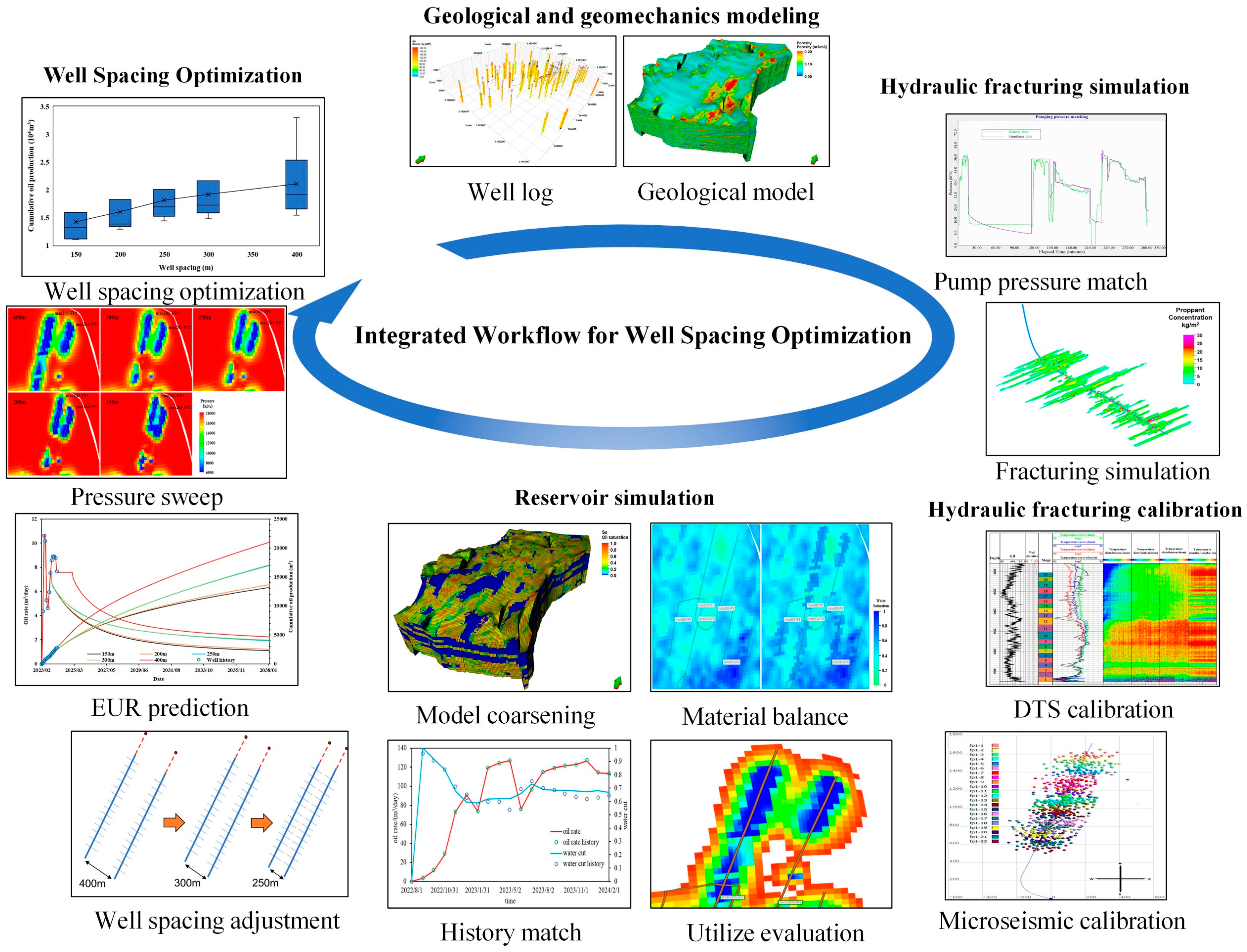
As shown in Figure 1, an integrated workflow has been established for optimizing the well spacing of tight oil wells, which includes detailed 3D geological and geomechanics modeling, precise dynamic fracture propagation simulation, hydraulic fracture field monitoring and analyses, and numerical reservoir simulation. We analyzed and evaluated the current degree of reservoir development and proposed different well spacing adjustment strategies. Through this integrated workflow, production forecasts and evaluations of different well spacing adjustment plans have been completed, determining reasonable well spacing for this block and guiding future development. Integrating actual seismic data from the field, well logging interpretation results, and core sampling data, a stochastic modeling method has been employed to construct a three-dimensional (3D) geological model and a 3D geomechanics model for the field. The 3D geological model, which accurately represents the reservoir’s initial properties, seamlessly integrates with the numerical reservoir simulator, while the 3D geomechanics model guides the simulation of fracture propagation by calibrating the mechanical parameters to better match actual geological property variations.
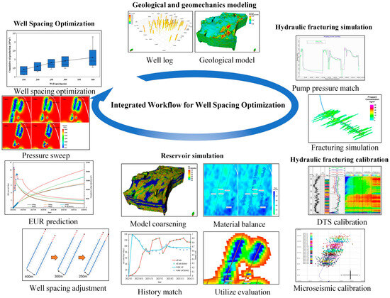
Figure 1.
Well spacing optimization workflow.
The accuracy of the simulated fractures heavily relies on the methodologies used during the simulation process [28,29]. Achieving both speed and precision in fracture simulation is quite challenging, and various fracture simulation methods provide different compromises between these two aspects. This study adopts the GOHFER hydraulic fracturing simulator, which is widely applied in the field. The simulator is based on a planar 3D model and demonstrates commendable performance in both the precision and speed of fracture simulation [30,31,32,33,34]. Lab fracture toughness testing is significantly influenced by the size and shape of the samples, which makes it impossible to scale up from the core scale to the actual field scale. The GOHFER simulator calculates fracture propagation based on the process zone stress (PZS) derived from direct field stress tests, ensuring higher accuracy and rationality than fracture toughness [35,36]. The calculation formula is as follows:
where , , and are process zone stress, instantaneous shut-in pressure, and closure pressure, respectively.
The propagation of the fracture can be determined based on the process zone stress (PZS) and the fracture net pressure:
where and are the fracture net pressure and the fracture criteria tolerance, respectively.
The net pressure is expressed by
where , , and are the fracture fluid pressure, minimum horizontal in situ stress, and pore pressure, respectively.
We also consider the pressure interference between fractures, and the stress shadow expression is as follows:
where , , and are the stress shadow, distance from the fracture face, and transverse exponent, respectively. The transverse exponent controls stress decay. The value of the exponent is 2 or less, with smaller values being more suitable for low-permeability reservoirs.
Furthermore, the simulation incorporates shear slip theory to couple rock fractures. Compared to traditional linear elastic fracture mechanics, it effectively prevents the overestimation of fracture heights and ensures that the simulation results match the actual geological conditions. Through the analysis of micro-seismic data and distributed temperature sensing monitoring in the field, combined with fracture propagation simulation results, clearer fracture parameters, such as fracture length and height, are determined. Then, the fractures are integrated with the numerical reservoir simulator through local grid refinement (LGR). Subsequently, we completed the history matching for all the wells, clarified the utilization of the reservoir, and analyzed the potential for well spacing adjustments. Then, we simulated the production dynamics of six wells within the block under five different well spacing strategies. Ultimately, we analyzed inter-well pressure interference and production characteristics to determine the optimal well spacing.
3. Geological and Geomechanics Modeling
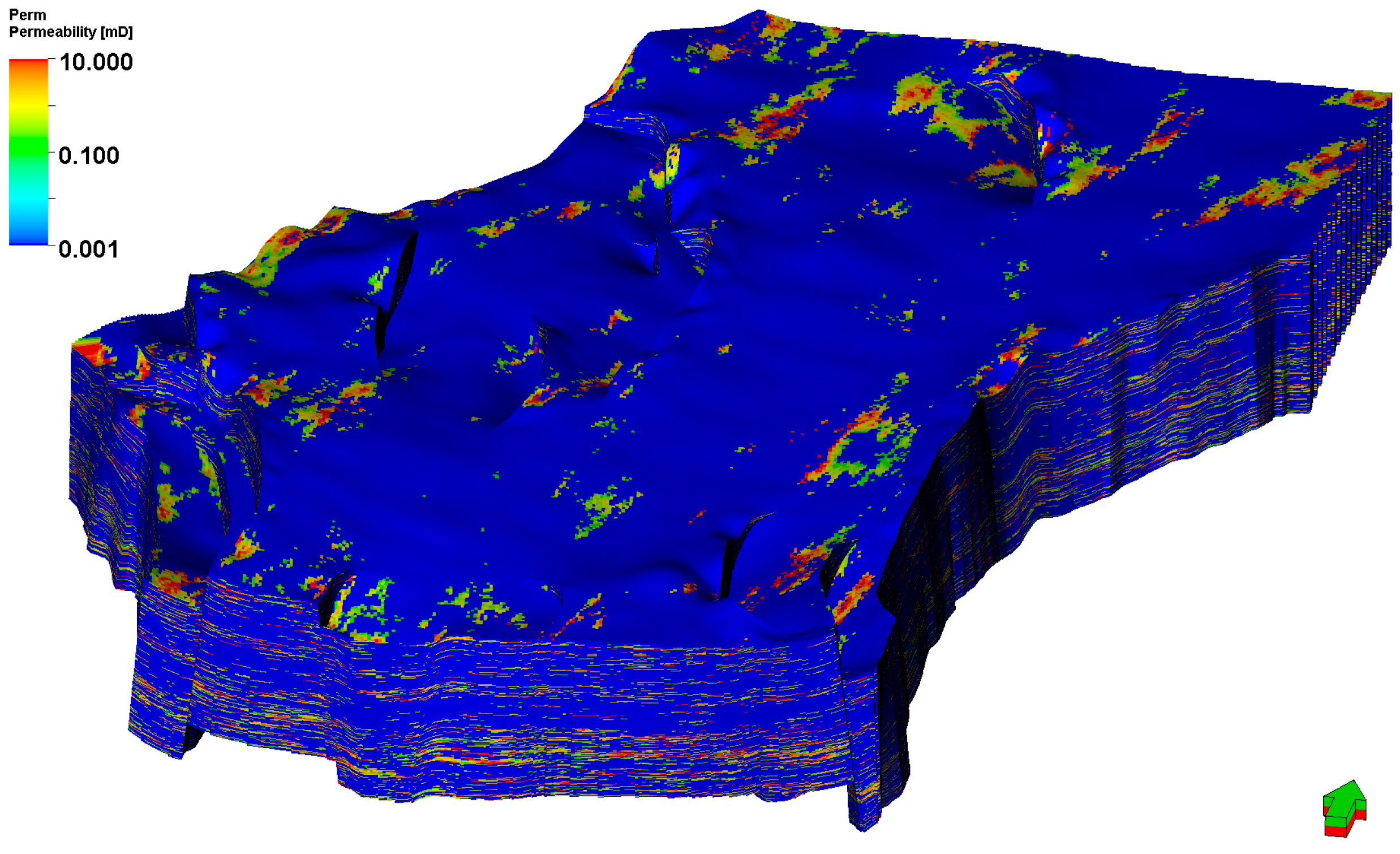
The 3D geological model is a concrete representation of the distribution of reservoir properties and their heterogeneity in three-dimensional space, and it is also the fundamental step in the integrated workflow. Based on the seismic data obtained from pilot exploration, the interpreted fault distribution, and stratigraphic data, the geological structural model was established. Combining well logging data interpretation results and core analysis results and integrating well and seismic data, a reservoir lithofacies model and property model were constructed. The property model includes models for porosity, permeability, oil saturation, and net-to-gross ratio. Figure 2 illustrates the permeability model for the entire area. There exists a transitional lithology with higher clay content between sandstone and shale. Consequently, we employed seismic data to constrain the model, effectively minimizing uncertainties inherent in stochastic modeling.
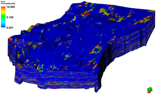
Figure 2.
Permeability model for the entire reservoir block.
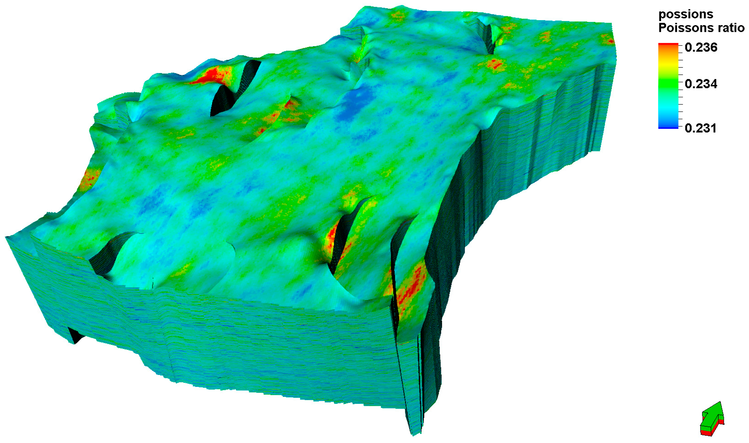
The 3D geomechanical model is a prerequisite for fracture propagation simulation and plays a decisive role in the geometry and properties of the simulated fractures. Similar to geological modeling, geomechanical modeling also starts with well log data and then expands to the entire area through stochastic simulation methods. The foundation for calculating the geomechanical parameters includes the P-wave and S-wave time differences and density curves obtained from well logging. According to the geomechanical calculation formulas, as shown in Table 1, a 3D geomechanical model of the work area’s Poisson’s ratio, Young’s modulus, maximum and minimum horizontal principal stresses, etc., has been established. The Poisson’s ratio model for the entire area is shown in Figure 3.

Table 1.
Geomechanical calculation formula.

Figure 3.
Poisson’s ratio model for the entire reservoir block.
Here, , , , , , , and are the P-wave velocity, S-wave velocity, rock density, vertical principal stress, pore pressure, tectonic strain coefficient, and Biot’s coefficient, respectively.
4. Hydraulic Fracturing Simulation
A hydraulic fracturing simulation was completed utilizing the GOHFER 3D (version 9.4.1, Halliburton, TX, USA) software. The geomechanical model established in the previous work was directly imported into the software, facilitating the construction of the fracturing model. Based on the analysis of mini-frac tests, we adjusted the leak-off coefficient and reservoir stress parameters. During the fracture propagation simulation, we took into account factors such as fracturing fluid loss, proppant transport, and stress shadowing caused by interference between fractures.
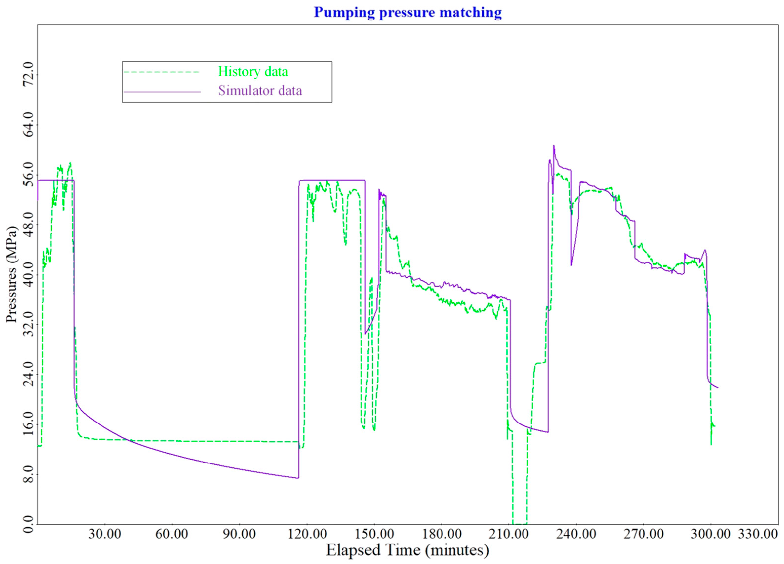
Given the mechanical characteristics of the block and the understanding from micro-seismic data, this study suggests that longitudinal fractures are rare or non-existent; hence, only transverse fractures were modeled. In the fracture propagation simulation, the well completion design and pumping schedule strictly matched the data provided in the field construction report. Figure 4 shows the pressure match result for the first stage of a horizontal well within the block. To enhance the computational speed of the simulation, a larger time step was selected, which made the simulated pressure curve appear smoother. The simulated pressure closely matched the actual data, significantly enhancing the credibility of the results.

Figure 4.
Pumping pressure matching. The dashed line represents actual pressure, while the solid line represents simulated pressure.
Taking the mao203-FP12 well within the field as an example, fracturing treatment was conducted over 21 stages. By integrating well logging data, completion data, and a pumping schedule, a dynamic simulation of the propagation of multi-stage, multi-cluster fractures was performed. The simulation results indicate the following key fracture parameters: an average fracture half-length of 224.15 m, an average propped fracture half-length of 154.67 m, and an average effective fracture height of 4.33 m. Additionally, the average proppant concentration within the fracture was 7.51 kg/m2, and the average fracture permeability was 99.16 md·m.
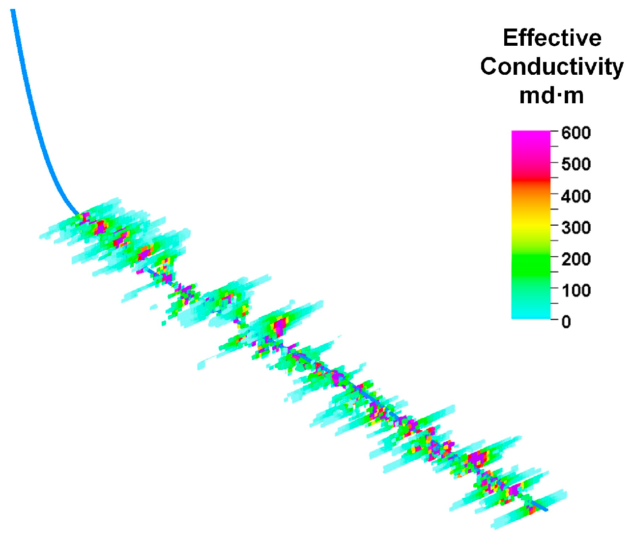
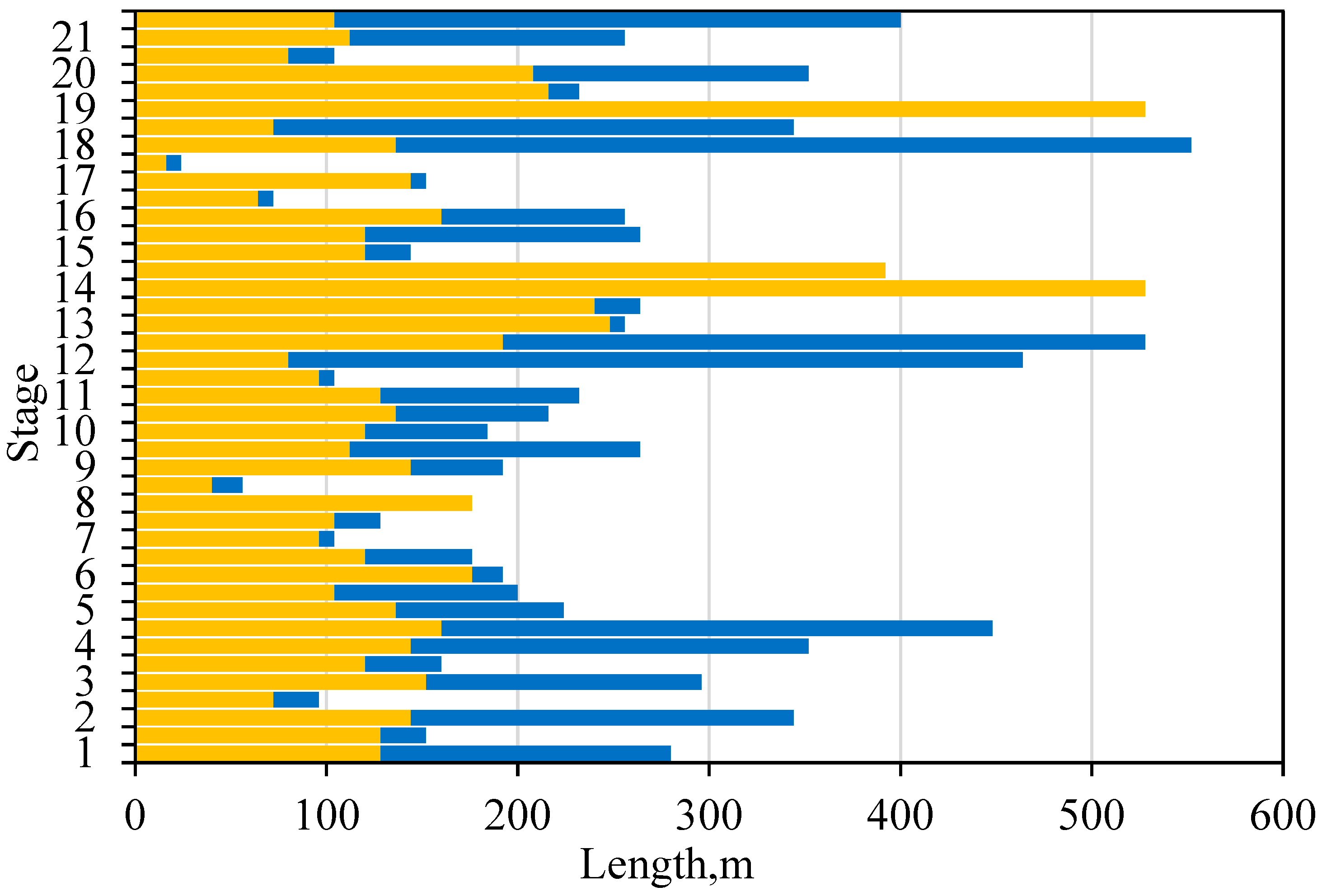
Simulated fractures are usually longer than the actual observed fractures. Figure 5 illustrates the distribution of the proppant concentration for all the fracture stages. Proppants are carried a significant distance by the fracturing fluid and have high concentrations near perforations, where the fractures are effectively propped, resulting in high conductivity. However, the concentration is lower near the fracture tips, which may not provide the necessary prop for the fracture to maintain conductivity. Figure 6 illustrates the effective conductivity of the fractures, which approximately decreases from the perforation to the tip of the fracture. The actual fractures that contribute to flow are shorter than those simulated. As depicted in Figure 7, by analyzing the effective propped fracture length and the length of the fracture that fracturing fluid can reach in this well, we can draw the same conclusion: the fractures that are propped and capable of providing conductivity are actually quite short, and they have often been overestimated in prior studies.
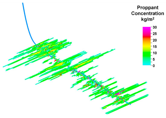
Figure 5.
Proppant concentration (kg/m2).
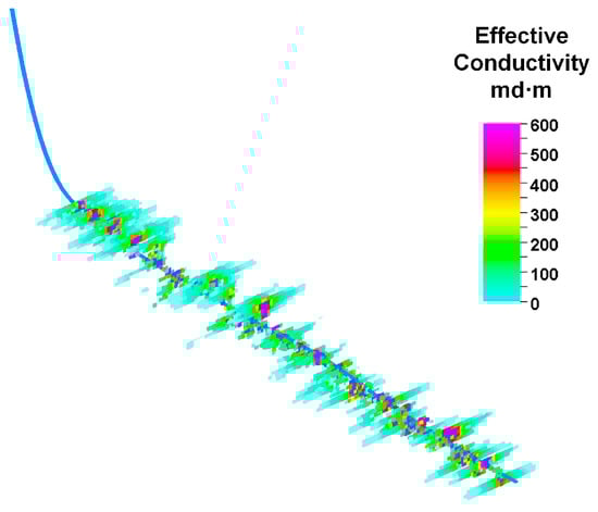
Figure 6.
Effective conductivity (md∙m).
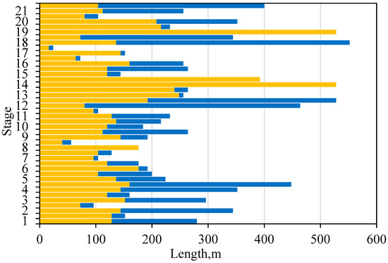
Figure 7.
The yellow in the bar chart represents the effective propped half-length of the fracture, while the blue represents the half-length of the fracture that the fracturing fluid can reach.
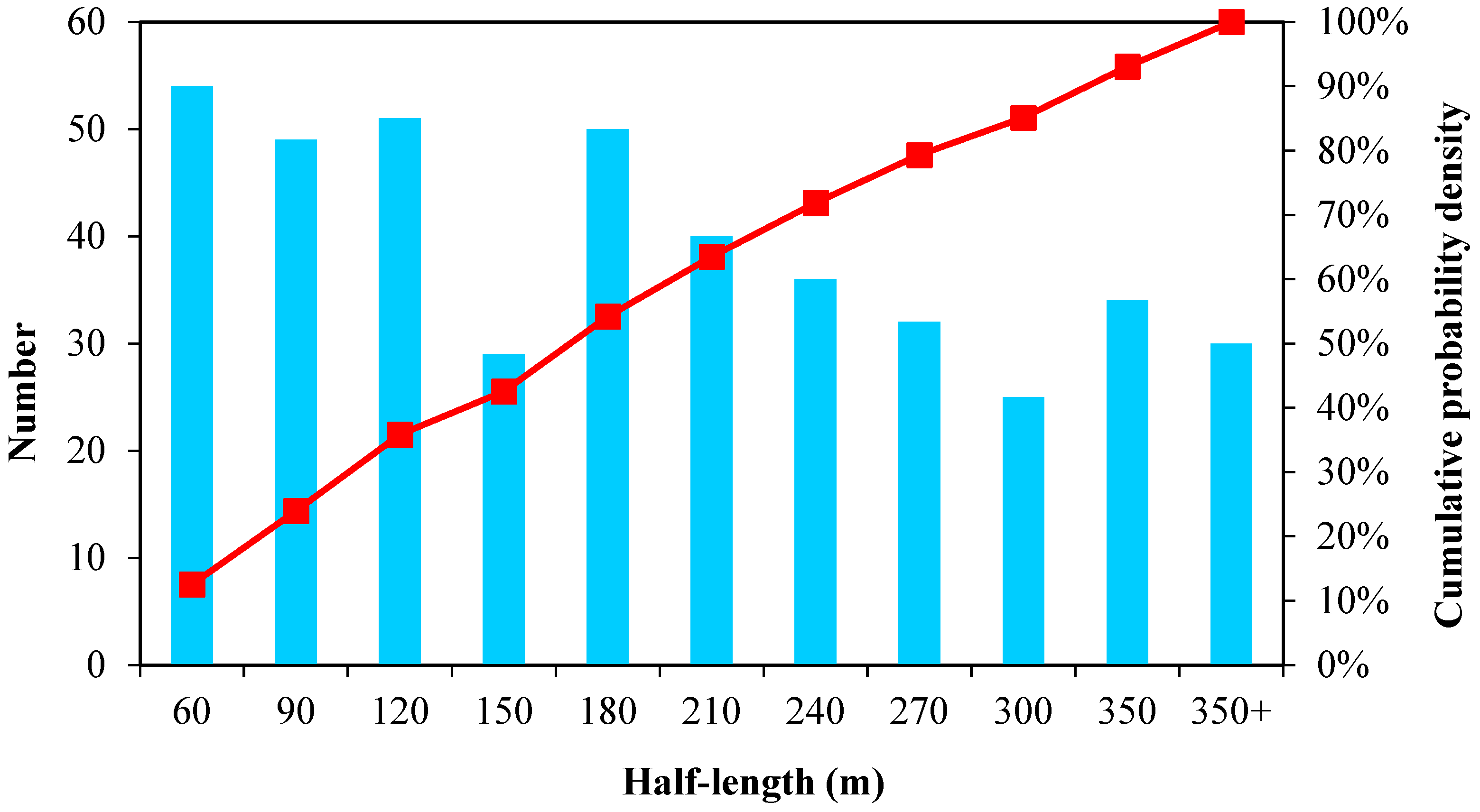
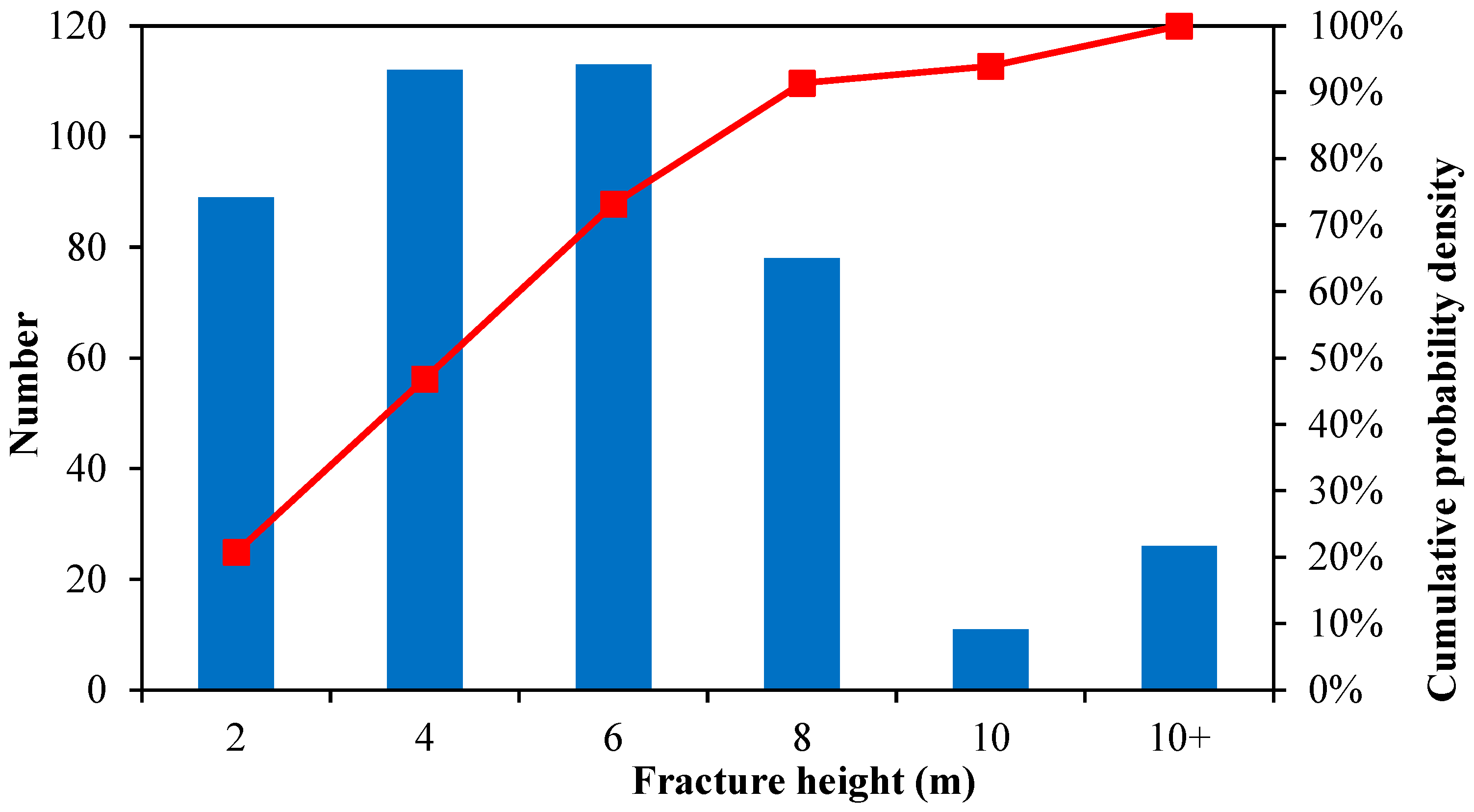
Therefore, we compiled the simulation results of fractures for all wells in the entire area. For each stage of each well, we analyzed the distribution pattern of representative fractures (the longer fractures in all clusters), as shown in Figure 8. The average half-length of fractures is 200 m, with 80% of fractures having a half-length of less than 300 m. The actual length of fractures with effective conductivity is less than the length that fracturing fluid can reach. As depicted in Figure 9, the height of the hydraulic fractures is generally less than 8 m for 90% of the stages. This is due to the presence of interbedded shale layers and their restrictive effect on the vertical propagation of fractures. The likelihood of fractures crossing layers in the simulation is quite low. However, if the well trajectory is intentionally designed to penetrate through two reservoir layers consecutively, some fractures may extend vertically through both layers. Nevertheless, the majority of fractures are confined to a single, thin layer.

Figure 8.
The bar chart represents the number of fractures with different half-lengths, while the line chart represents the cumulative probability density.

Figure 9.
The bar chart represents the number of fractures with different half-heights, while the line chart represents the cumulative probability density.
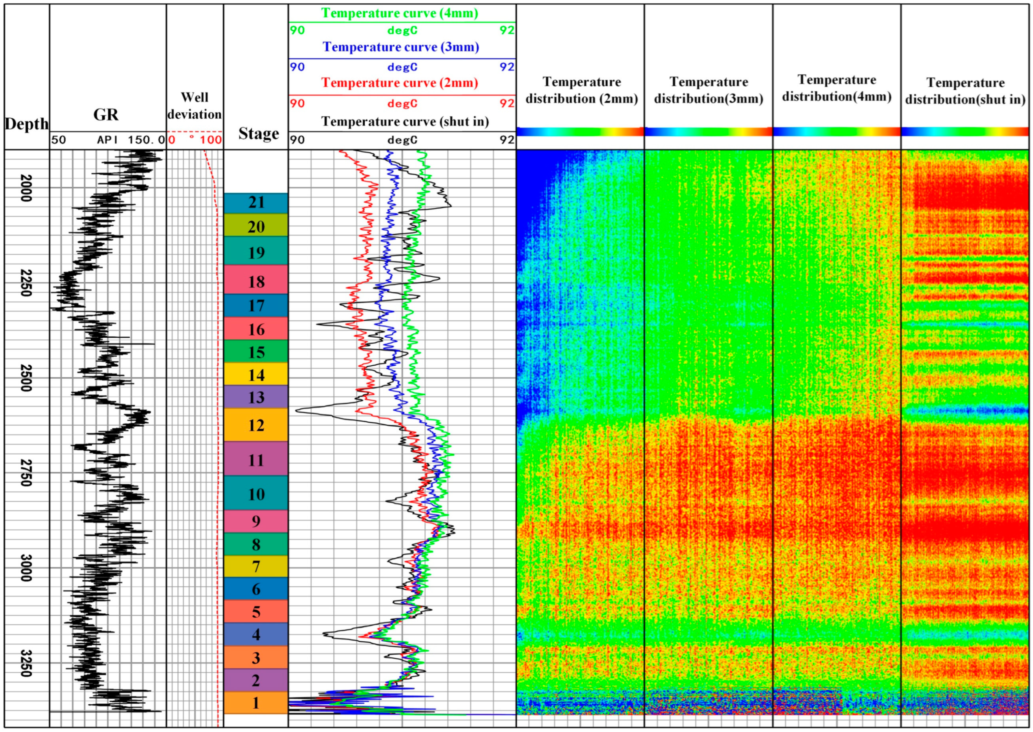
In this study, the field employed a variety of techniques to monitor the multi-stage, multi-cluster hydraulic fracturing of horizontal wells, including micro-seismic monitoring and fiber-optic fluid production testing. Specifically, the mao203-FP12 well was subjected to distributed temperature sensing (DTS) monitoring. The testing was conducted six months after the well was fractured and brought into production. Surface fluid production and downhole temperature distribution were measured under different oil nozzle diameters of 2 mm, 3 mm, and 4 mm. Monitoring was carried out for 12 h at each oil nozzle diameter from small to large, and finally, the well was shut in for monitoring. By modeling and calculating the surface production and temperature data, the production of different fracture clusters was determined. Quantitative calculations were performed using the stable temperature profiles at later stages for each size (temperature fluctuations less than 0.5 °C within 30 min).
Figure 10 displays the gamma ray (GR) log curve of the horizontal section of the well and the temperature curves and distribution heat maps for different fracturing stages under different oil nozzle diameters. The calculation results show that the liquid production characteristics are directly related to the oil nozzle diameter. As the oil nozzle diameter increases, the number of productive fracture stages gradually increases. The main liquid production comes from stages 2 to 6, 13 to 14, and 17 to 18. The GR log curve indicates that these productive stages have lower values, suggesting a higher content of sandstone, signifying better reservoir quality.
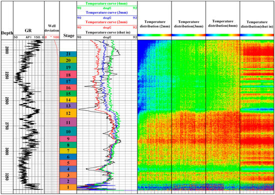
Figure 10.
DTS curve and heat map at different oil nozzle diameters in the fracturing stages of the mao203-FP12 well.
Typically, the Pearson product–moment correlation coefficient is used to analyze the correlation (linear relationship) between two variables, with values ranging between −1 and 1. In this context, the coefficient is employed to examine the relationship between the results of hydraulic fracturing operations and the outcomes from distributed fiber-optic monitoring. The formula for the Pearson product-moment correlation coefficient is provided as follows:
where , and are the mean of , the mean of , and the total number of observations, respectively.
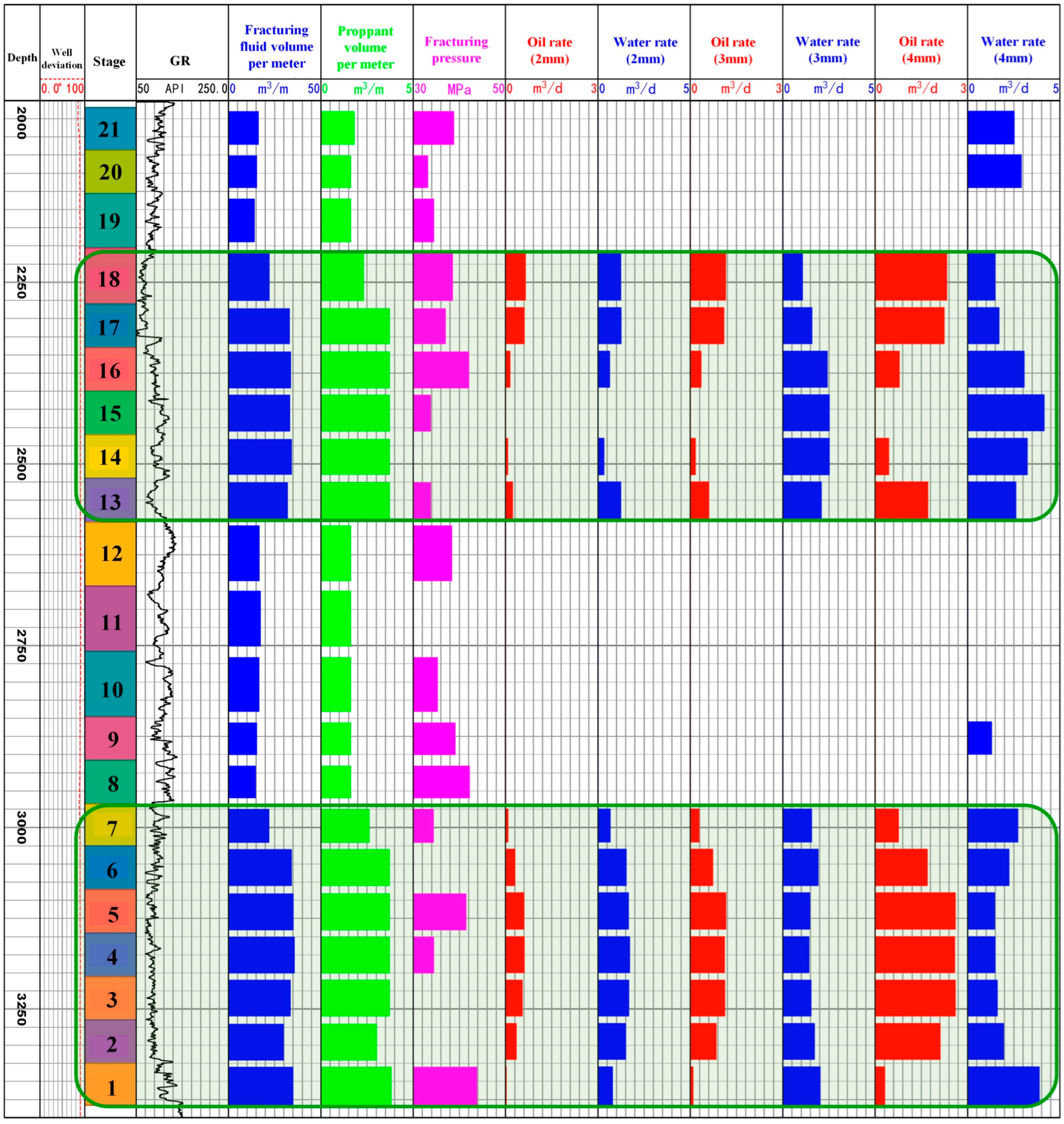
As shown in Figure 11, a comparison is made between the hydraulic fracturing simulation results and the results from DTS testing for the mao203-FP12 well. The differences in the liquid production capacity of each stage are more significantly correlated with the proppant concentration within the fractures and the volume of the fracturing fluid. For this well, the proppant concentration () and the volume of fracturing fluid () show a more pronounced correlation with the ultimate liquid production capacity.
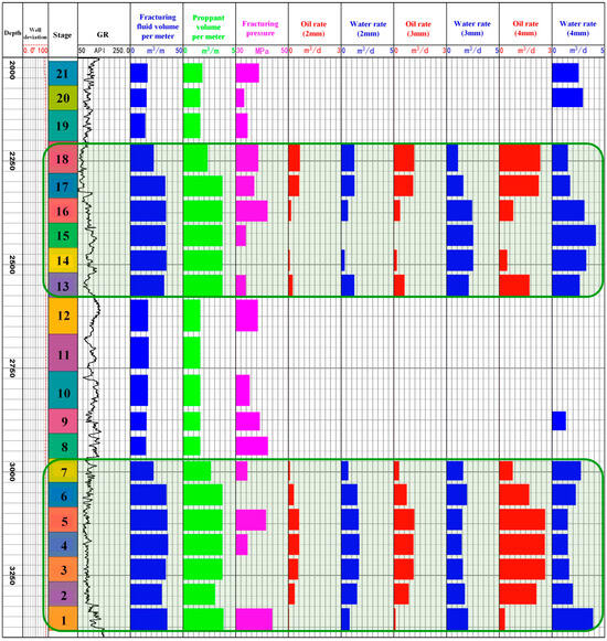
Figure 11.
Bar chart comparing the fracturing liquid volume, proppant volume, and rock breakdown pressure of each stage in the fracturing treatment of the mao203-FP12 well with the oil and water production rate calculated by DTS monitoring.
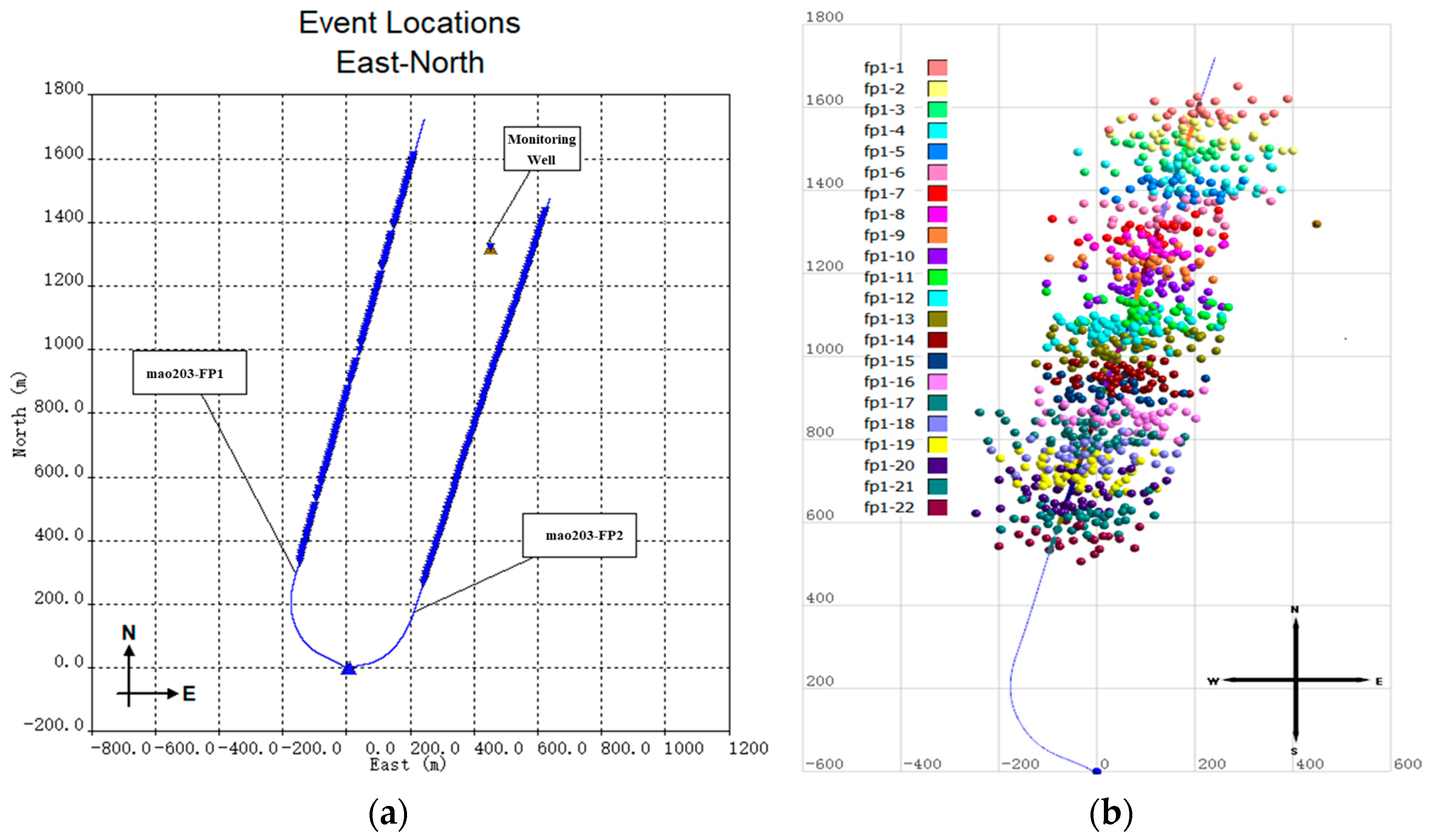
During the hydraulic fracturing treatment of the mao203-FP1 well, micro-seismic monitoring was conducted through its adjacent well, as shown in Figure 12a. The monitoring well for the fracturing of mao203-FP1 is the mao203-1 well, which is located to the northeast of it. The bridge plug of the monitoring well is at a depth of 1900 m, with the geophone positions ranging from 1780 to 1890 m. The fracturing operations of stages 1 to 22 of the mao203-FP1 well were monitored, with the monitoring distances ranging between 320 m and 590 m. Figure 12b displays the micro-seismic events detected on both sides of the mao203-FP1 well. A total of 876 micro-seismic events were interpreted, with the fracture half-length ranging from 138 m to 212 m and an average fracture half-length of 172 m, indicating poor symmetry between the two wings of each fracture stage. The azimuth of the fracture network is between NE77° and NE105°, with an average of NE90°, which is essentially perpendicular to the well trajectory direction. We utilized the multi-stage, multi-cluster dynamic fracture propagation simulation method for this well. The numerical simulation results also indicate that the hydraulic fractures are approximately perpendicular to the wellbore. The simulation yielded an average half-fracture length of 166.72 m and an average effective fracture height of 7.54 m for the mao203-FP1 well. The discrepancy between the fracture lengths from the simulation and those from micro-seismic monitoring is relatively small. Additionally, in this study, when comparing micro-seismic data with the results of fracture propagation simulation, it was observed that the fracture height detected by micro-seismic monitoring is much larger than that obtained from the simulation, approximately three times. Based on the analysis of Figure 9 and field knowledge, we believe that the possibility of fractures crossing layers is very low, and the fracture height interpreted from micro-seismic data is excessively high.
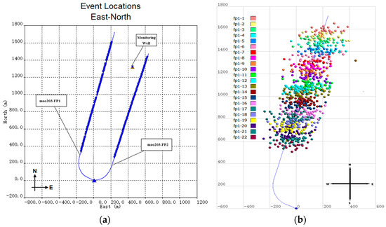
Figure 12.
Here, (a) is the location of the micro-seismic monitoring well and the monitored well, and (b) is the distribution of micro-seismic events detected from stage 1 to stage 22 of the mao203-FP1 well.
By analyzing the DTS data and micro-seismic data, we can, to some extent, eliminate the uncertainty in the fracture geometry and properties obtained from fracture simulation. However, this benefit is relative because there are inherent uncertainties in both fiber-optic testing and micro-seismic testing. In subsequent history matching during numerical reservoir simulation, the fracture simulation results can be further adjusted based on the well’s production performance. This process will minimize uncertainty as much as possible and provide reliable data for well spacing optimization.
5. Reservoir Simulation
To accurately portray the properties of the reservoir and minimize the errors caused by interpolation when establishing property models, reservoir 3D geological models are typically very detailed. When performing numerical reservoir simulation, a large number of grids do not bring significant advantages to the final results; instead, they increase the load on the simulator, leading to slow computation speeds. Therefore, using a detailed geological model for numerical simulation is not optimal in terms of time efficiency and economic returns. To solve this problem, it is necessary to coarsen the geological model.
To ensure the original properties of the reservoir and reduce coarsening errors in the planar and vertical directions, property-constrained coarsening methods are commonly used. As shown in Table 2, a net-to-gross ratio constraint is often used when determining the coarsening porosity. For oil saturation, both net-to-gross ratio and porosity constraints are typically applied. Permeability and net-to-gross ratio are usually not constrained. These methods effectively avoid the problem of non-reservoir formations becoming reservoirs after coarsening operations, which leads to a significant increase in geological reserves. As depicted in Figure 2, the original model consisted of 190 layers with 19.13 million grids, with a modeling precision of 25 m × 25 m × 1 m; after coarsening, it contained 13 layers with 538,000 grids, with a modeling precision of 50 m × 50 m × (13~17 m).
Table 2.
Coarsening constraint conditions.
In this work, the IMEX module, a black oil simulator within the CMG suite of numerical reservoir simulation (version 2022.10, Computer Modelling Group, Calgary, Canada) software, was utilized. The coarsened geological model was seamlessly integrated with the numerical reservoir simulator. Basic settings were completed based on fluid PVT parameters and relative permeability parameters obtained from laboratory tests. Table 3 shows the basic parameter table of numerical reservoir simulation. A single porosity model was adopted, and non-equilibrium initialization was used. The reserves calculated after initialization were found to be consistent with those calculated using the geological model.
Table 3.
Basic parameter table of numerical reservoir simulation.
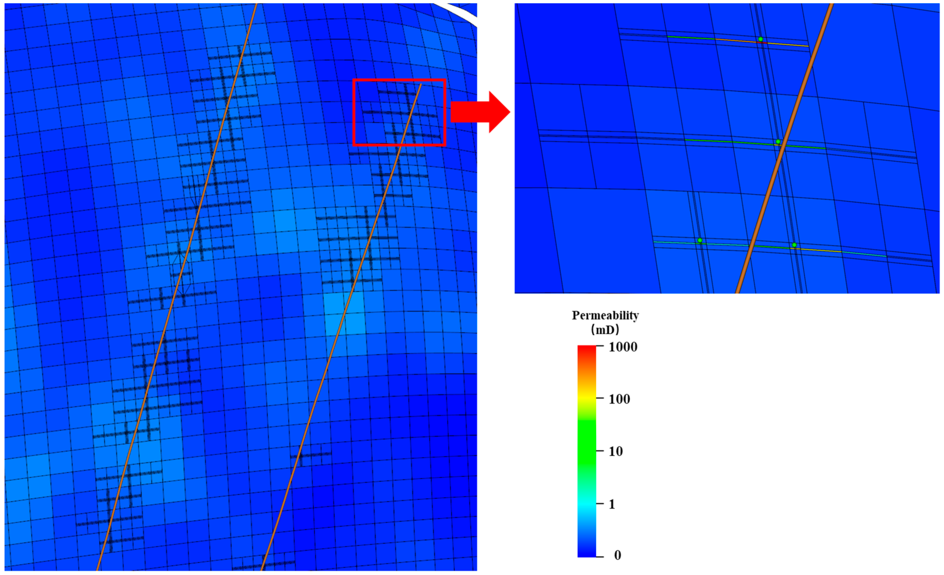
The results of the fracture propagation simulation were seamlessly integrated with the numerical reservoir simulator through standardized keywords, as shown in Figure 13. In the numerical reservoir simulator, a method of local grid refinement was used to represent the fractures and fracture parameters were stored in keyword arrays. Subsequent tasks, such as history matching, can be directly modified within the corresponding keyword arrays. Based on field monitoring results, when interfacing with the numerical simulator, the permeability or flow capacity cutoff values were set to remove unpropped ineffective fractures, ensuring that the fractures used in the numerical reservoir simulation are more realistic.
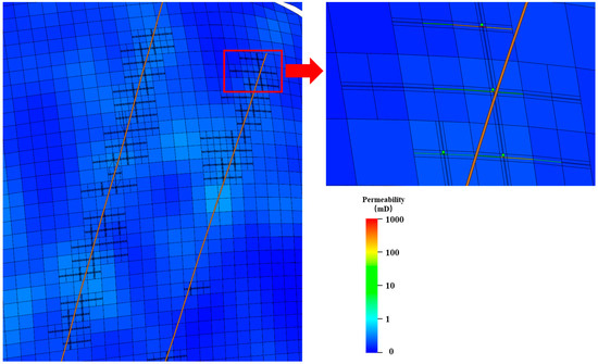
Figure 13.
Local grid refinement for hydraulic fractures.
When considering the leak-off of fracturing fluid, we calculated the volume of the fracture control area and collected data on the volume of fracturing fluid pumped into each well. Based on the principle of material balance, the original oil saturation and porosity were modified to truly reflect the distribution of oil and water in the formation after large-scale, multi-stage hydraulic fracturing.
This study treats the fracturing fluid as a component with properties identical to water, so the injection of fracturing fluid is equivalent to water injection. Based on the principle of material balance, a relationship between the pore volumes before and after fracturing can be established:
where , , and are the pore volumes before and after fracturing and the fracturing fluid volume, respectively.
After hydraulic fracturing, the porosity within the stimulated reservoir volume changes. In addition to the original oil and water, the pores also contain the injected fracturing fluid. Therefore, the porosity multiplier can be calculated using the following formula:
where and are the porosity before and after fracturing, respectively.
Correspondingly, the oil saturation and water saturation within the reservoir also change, and their multipliers can be calculated as follows:
where , , and are water saturation before and after fracturing and oil saturation before fracturing.
Table 4 illustrates the property values before and after the material balance for a well within the block. The calculation process consists of three steps:
Table 4.
Material balance calculation.
The well’s initial properties within the stimulation area are statistically recorded, including the initial pore volume, oil volume, water volume, average porosity, and average permeability, as well as the fracturing treatment data. The mao203-FP1 well completed a total of 25 fracturing stages, with 35,488 cubic meters of fracturing fluid being injected.
Subsequently, using the fracturing fluid injection data and applying Formulas (6)–(9), the post-fracturing pore volume and the volumes of oil and water can be calculated, which in turn enables the determination of the change multipliers for each property.
Lastly, these property multipliers are applied to modify the initial properties of each grid in the numerical reservoir simulation.
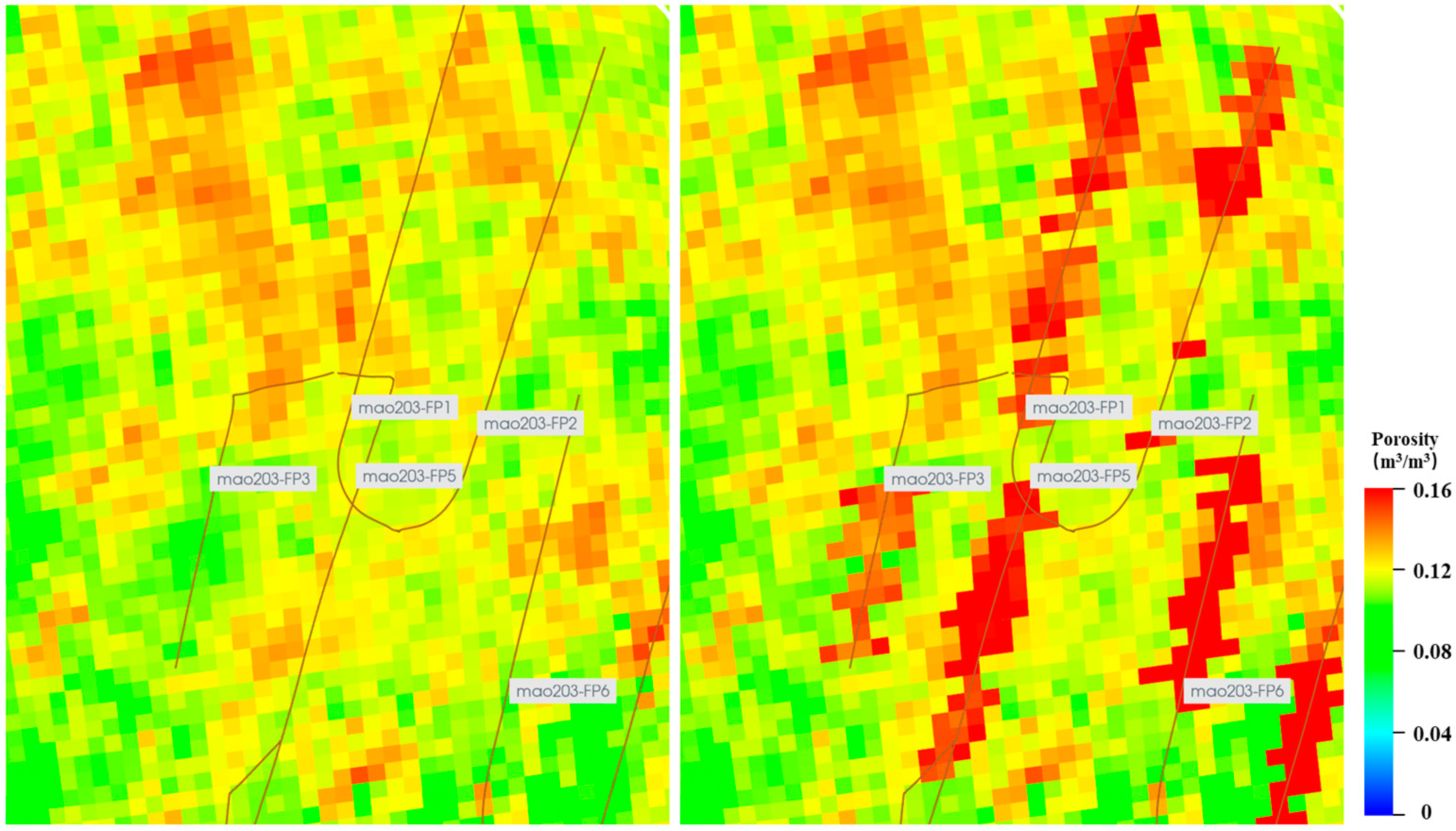
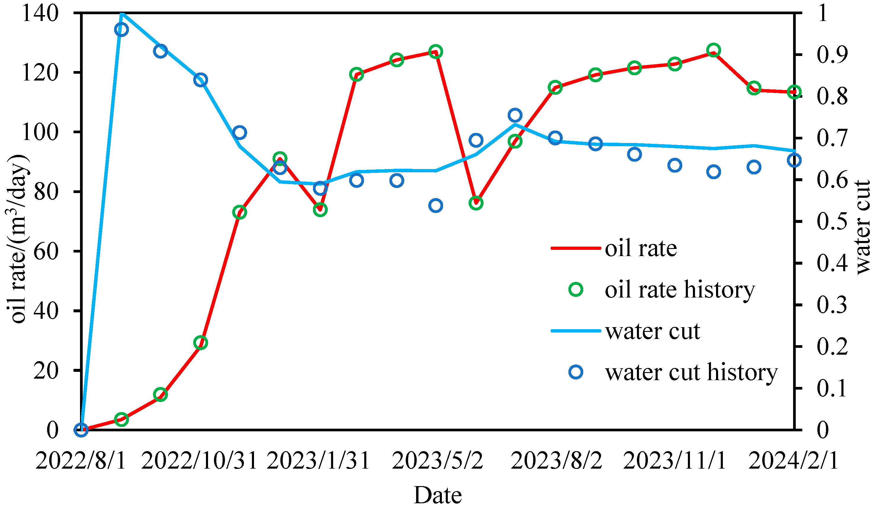
Figure 14 and Figure 15 show the models of water saturation and porosity before and after the material balance calculations. After considering the distribution of oil and water in the reservoir after hydraulic fracturing with material balance, the matching of water cut during the early production of the oil well became easier. A calibrated model was used to complete the history matching of single wells and the entire field. As shown in Figure 16, we constrained the oil production rate to match the bottom hole pressure and water cut, and the matching effect was credible.
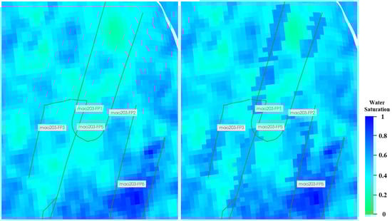
Figure 14.
Water saturation model before (left) and after (right) material balance treatment accounting for fluid leak-off.
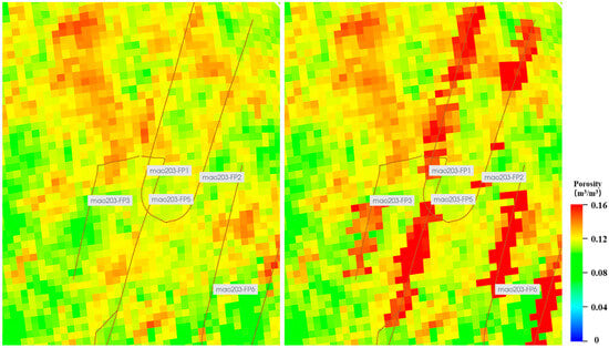
Figure 15.
Porosity model before (left) and after (right) material balance treatment accounting for fluid leak-off.
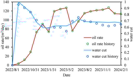
Figure 16.
History match results of the oil production rate and water cut of the whole reservoir block. Circle dots are observed data, while the solid lines denote history-matched results.
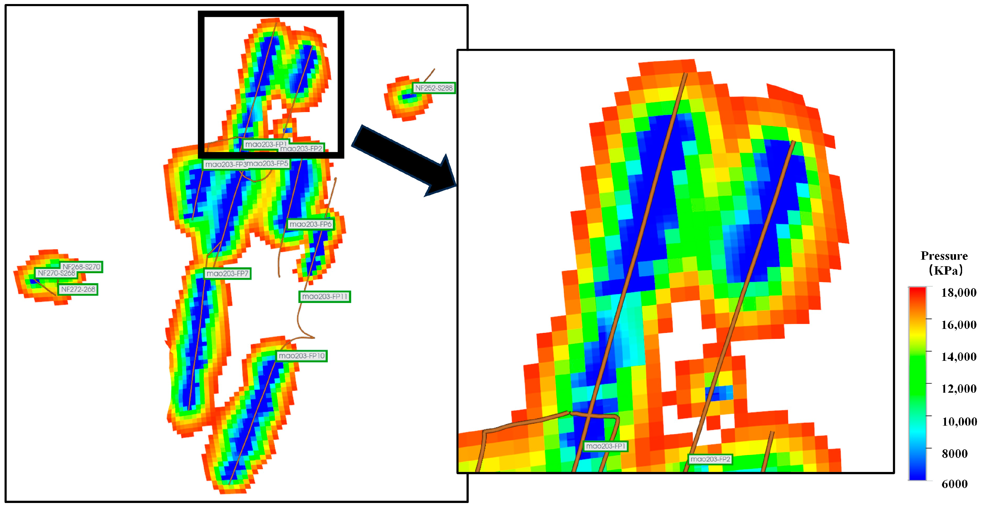
Previous studies completed the history matching for the entire field. Based on the credible history matching, a forecast was made for the estimated ultimate recovery for all wells in the block over a 15-year production period, and the utilization of the reservoir was clarified according to the pressure wave propagation. Figure 17 shows the pressure wave propagation after 15 years of production in the main FⅡ3 layer. The blue area near the wellbore can be approximated as the stimulated reservoir volume. This area has low remaining pressure and a high degree of drainage efficiency because the permeability has increased significantly after hydraulic fracturing, making oil and water flow easier. The green and yellow areas indicate pressure propagation, but due to the permeability not being as large as in the stimulated area, the degree of utilization is lower, and red indicates areas that are unutilized or almost unutilized. Overall, for the horizontal and vertical wells within the block, under the current well spacing, there is almost no pressure interference between wells, which will not affect the oil production capacity. The well spacing is relatively large, indicating potential for further optimization.

Figure 17.
The pressure wave propagation after 15 years of production in the main FⅡ3 layer. The enlarged section shows the pressure distribution between the two wells, with high residual pressure.
6. Well Spacing Optimization
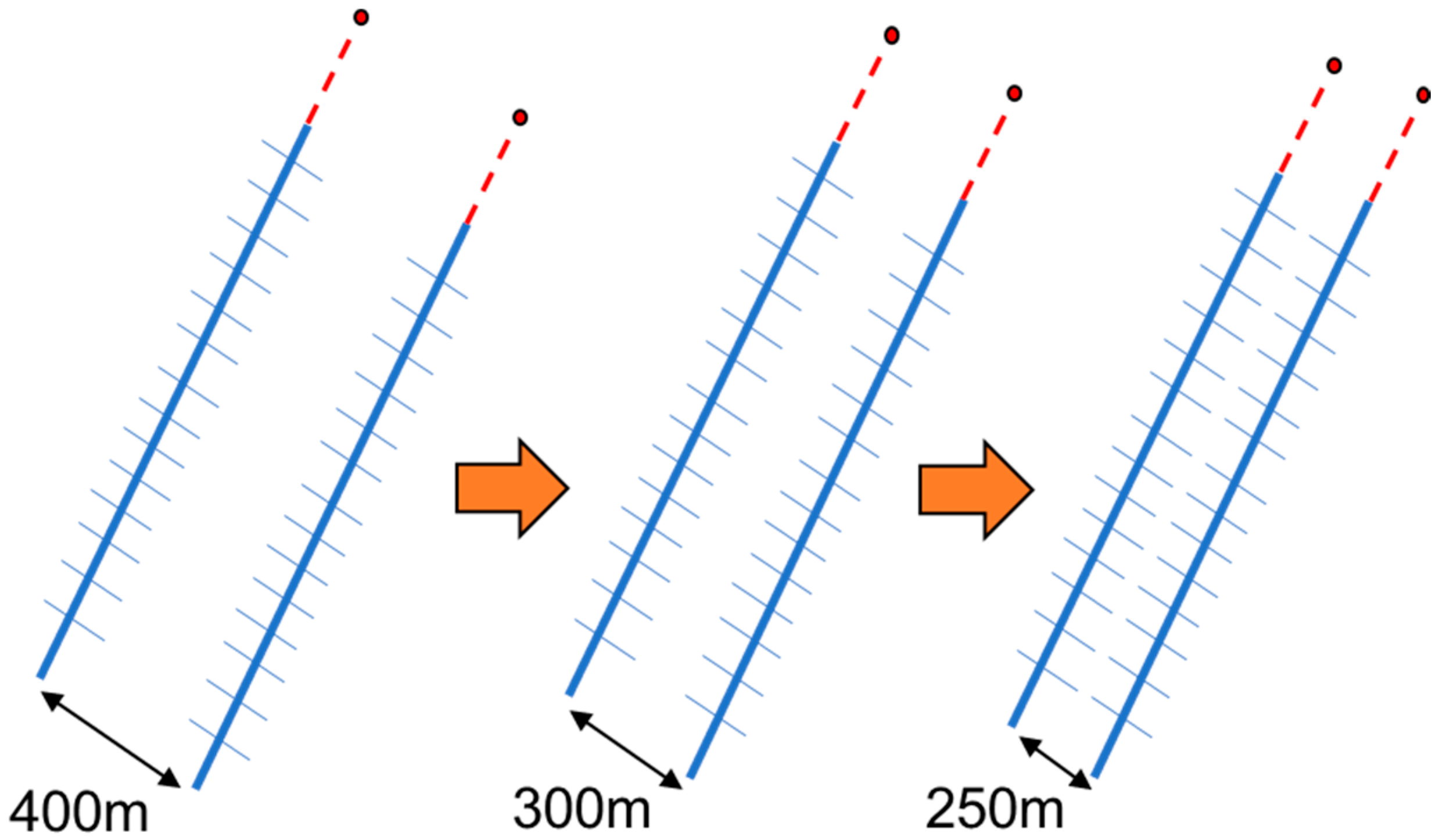
To determine the optimal well spacing in this area, which is to achieve the highest economic returns with minimal interference between wells, a study was conducted on three pairs of horizontal wells, totaling six wells, in the two main oil-producing layers within the block. This study aimed to provide a reference for the design of subsequent development plans. Since the horizontal wells in the block are approximately parallel, the initial well spacing was 300–400 m. When studying the spacing between two adjacent wells, one well was kept stationary while the other was translated along its direction to reduce the spacing to different distances, as shown in Figure 18. To eliminate potential uncertainties, the hydraulic fractures of the translated well, as well as its operating conditions and constraints, were made identical to those of the well before translation. The production performance of each well was simulated at well spacings of 150 m, 200 m, 250 m, 300 m, and 400 m, clarifying the production characteristics and the extent of inter-well utilization.

Figure 18.
Schematic diagram of well spacing adjustment.
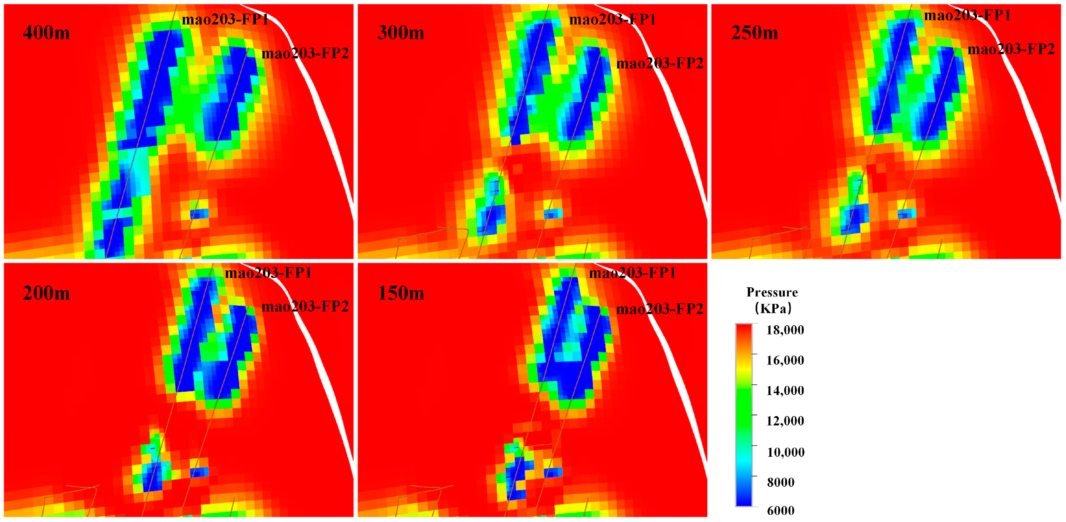
The mao203-FP1 and mao203-FP2 wells are two horizontal wells in the same layer. Due to the undulation of the strata, the fractures of the mao203-FP2 well penetrate vertically through layers. Figure 19 sequentially displays the pressure distribution after 15 years of production at different well spacings. When the well spacing was greater than 300 m, there was no interference between wells after 15 years of production; as the well spacing decreased below 300 m, the interference increased with the reduction in spacing. At a well spacing of 150 m, the interference was severe, and the remaining pressure between wells was low.
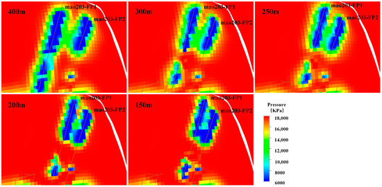
Figure 19.
The pressure wave propagation of the mao203-FP1 and mao203-FP2 wells after 15 years of production at different well spacings.
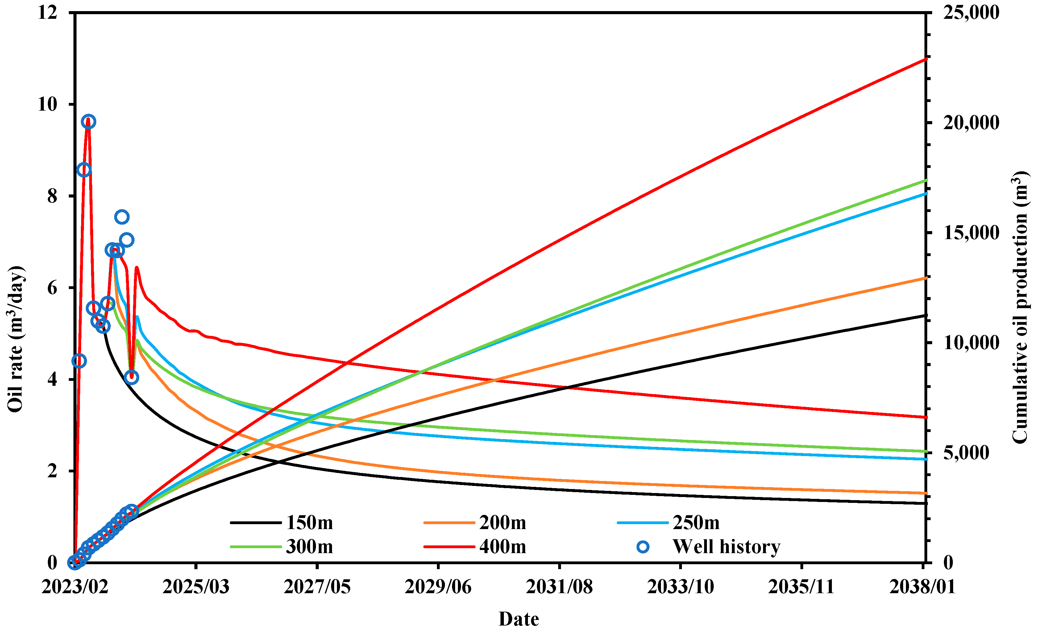
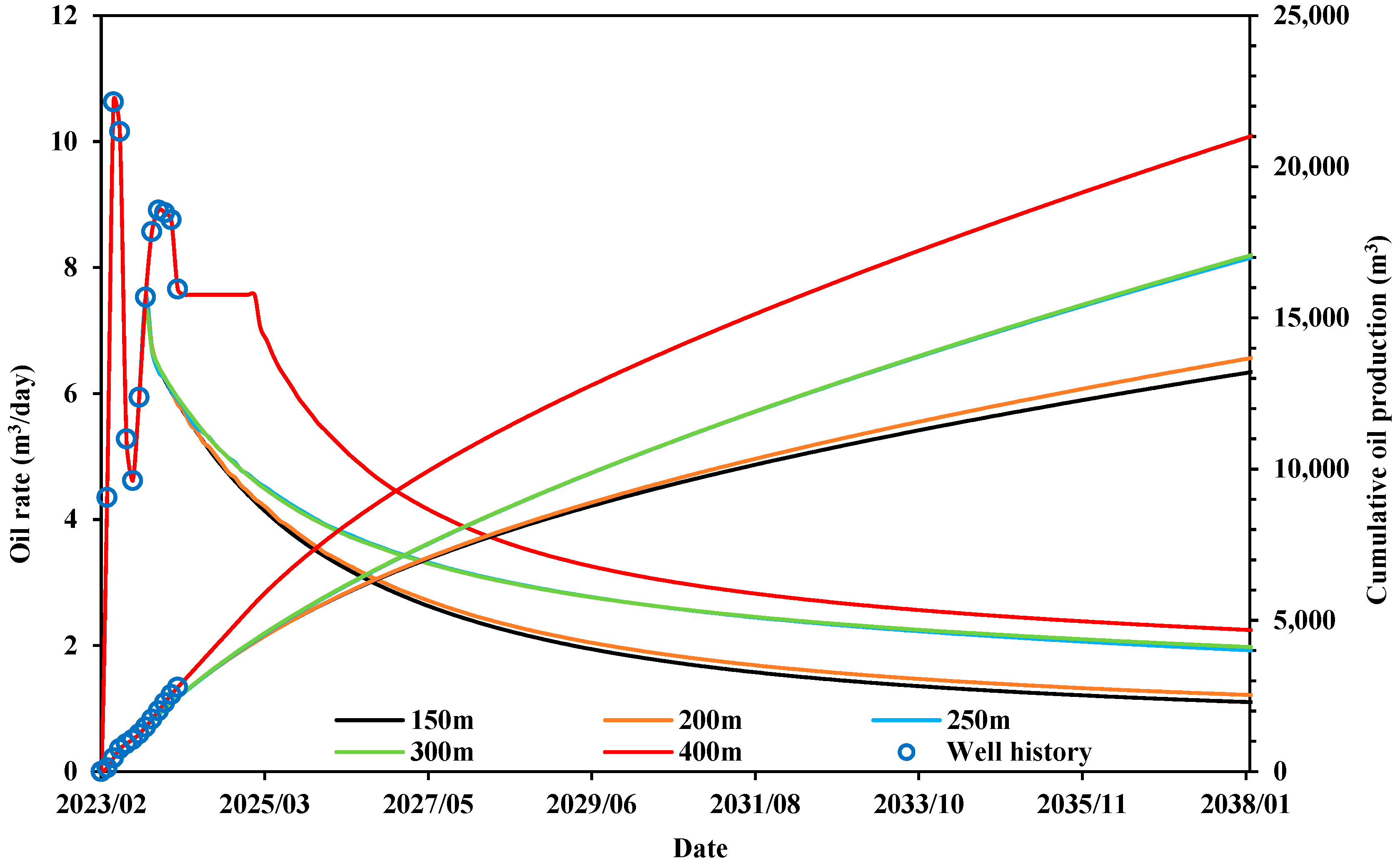
The oil production rate curves and cumulative oil production curves for the mao203-FP1 well at different well spacings are shown in Figure 20. For the mao203-FP1 well, the oil production rates and the cumulative oil volumes were almost identical across different well spacings during the first half-year of production.

Figure 20.
Oil production rate and cumulative oil production curve of the mao203-FP1 well at different well spacings.
As development progressed, the oil production rate gradually decreased, and after the well spacing fell below 250 m, both the oil production rate and cumulative oil production dropped significantly. During well position adjustments, the location of the mao203-FP1 well did not change; the main reason for the subsequent decline in oil production capacity was the severe interference that occurred between the two wells.
Similarly, as shown in Figure 21, the mao203-FP2 well exhibits the same characteristics as the mao203-FP1 well after adjusting well spacing, but there are still some differences due to its location change. At the initial well spacing, the oil production rate and cumulative oil volume were the highest because there was no interference between the wells. When the well spacing was either 300 m or 250 m, the rates were almost identical, indicating that in these spacings, there was no interference or the interference was minimal. At well spacings of either 200 m or 150 m, there was little difference in oil production rates and cumulative oil volumes, but compared to the initial well spacing, the production decreased by nearly 44.2%.
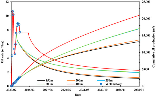
Figure 21.
Oil production rate and cumulative oil production curve of the mao203-FP2 well at different well spacings.
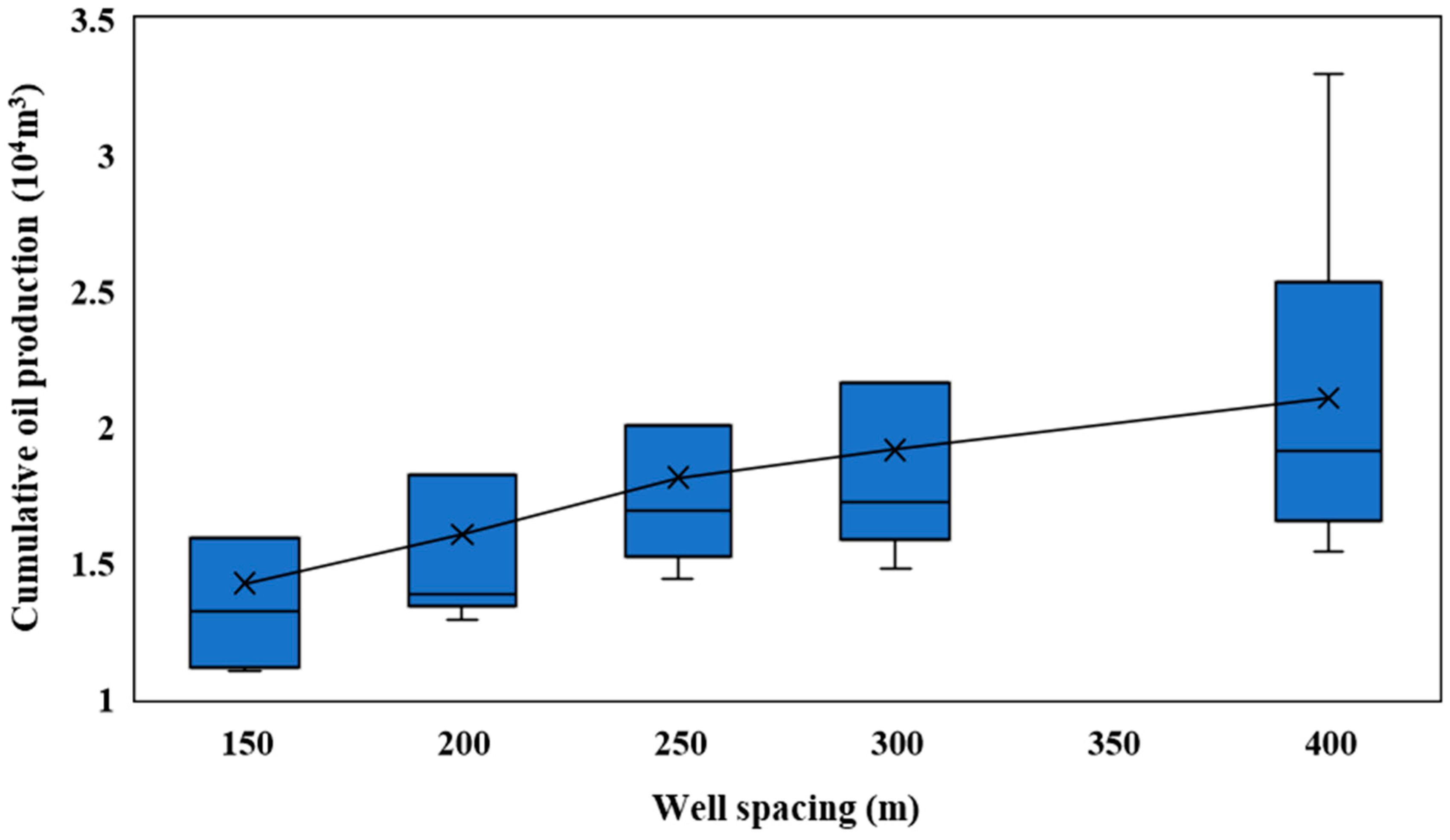
As shown in Table 5, we statistically analyzed the cumulative oil production of six horizontal wells over 15 years at various well spacings and presented our results in a box plot, as depicted in Figure 22. When the spacing between horizontal wells was 150 m or less, the 15-year cumulative oil production decreased by more than 35% compared to the initial well spacing. However, at a well spacing of 250 m, the production loss over 15 years was only approximately 10% of the cumulative oil production that would be achieved with the initial well spacing over the same period. At this spacing, although there was a reduction in production, the wells were nearly fully utilized with minimal remaining oil, indicating a more complete development. It was concluded that 250 m well spacing can be considered a reasonable development interval.
Table 5.
Cumulative oil production over 15 years at various well spacings.

Figure 22.
Box plots of the 15-year cumulative oil production for six wells with various well spacings.
7. Conclusions
In this study, we established an efficient integrated workflow to accomplish well spacing optimization, and the following conclusions were drawn:
- (1)
- Through pump schedule matching, field monitoring analysis, and production history matching, we ensured the reliability of the simulation results. Considering the leak-off of fracturing fluid through material balance, we simulated the production performance of six wells under different well spacings.
- (2)
- In general, the EUR of wells decreases as the well spacing is reduced. When the well spacing is less than 250 m, there is significant interference between wells, leading to a rapid decline in production. The reasonable well spacing is 250 m.
- (3)
- The current well spacing is too large, and the well pattern infill requires further deliberation. According to the optimized reasonable well spacing, infill drilling carries significant risks. It is recommended that in the subsequent development, the “one-time well pattern” should be taken seriously.
- (4)
- The integrated workflow can greatly enhance the efficiency of tight oil well spacing optimization, and the optimization results are highly reliable. Through this integrated workflow, a variety of optimization designs can be conducted, such as well pattern optimization, hydraulic fracturing optimization, and production optimization.
Author Contributions
Methodology, X.W.; software, W.W.; validation, W.W., X.W. and Z.S.; formal analysis, G.S.; investigation, H.Z.; data curation, G.S. and H.Z.; writing—original draft, W.W.; writing—review and editing, W.W., G.S., X.W. and Z.S.; visualization, W.W.; supervision, H.Z. and Z.S.; funding acquisition, X.W. All authors have read and agreed to the published version of the manuscript.
Funding
This work was supported by the National Natural Science Foundation of China (No. 52204060) and the Science Foundation of China University of Petroleum-Beijing (No. 2462021YJRC010).
Data Availability Statement
The original contributions presented in this study are included in the article. Further inquiries can be directed to the corresponding author.
Conflicts of Interest
Author Gangxiang Song was employed by Shanghai Branch of CNOOC Ltd. Author Hui Zhang was employed by Exploration and Development Research Institute, Petrochina Daqing Oilfield Company Ltd. The remaining authors declare that the research was conducted in the absence of any commercial or financial relationships that could be construed as a potential conflict of interest.
Nomenclature
| Process zone stress, MPa | |
| Instantaneous shut-in pressure, MPa | |
| Closure pressure, MPa | |
| Fracture net pressure, MPa | |
| Fracture criteria tolerance | |
| Fracture fluid pressure, MPa | |
| Minimum horizontal in situ stress, MPa | |
| Pore pressure, MPa | |
| Stress shadow, Pa | |
| Distance from the fracture face, m | |
| Transverse exponent | |
| P-wave velocity, m/s | |
| S-wave velocity, m/s | |
| Young’s modulus, GPa | |
| Rock density, kg/m3 | |
| Vertical principal stress, MPa | |
| Pore pressure, MPa | |
| Pore volume before fracturing, m3 | |
| Pore volume after fracturing, m3 | |
| Fracturing fluid volume, m3 |
References
- Sun, L.; Zou, C.; Jia, A.; Wei, Y.; Zhu, R.; Wu, S.; Guo, Z. Development characteristics and orientation of tight oil and gas in China. Pet. Explor. Dev. 2019, 46, 1073–1087. [Google Scholar] [CrossRef]
- Boak, J.; Kleinberg, R. Shale gas, tight oil, shale oil and hydraulic fracturing. In Future Energy; Elsevier: Amsterdam, The Netherlands, 2020; pp. 67–95. [Google Scholar] [CrossRef]
- Zhu, R.; Zou, C.; Mao, Z.; Yang, H.; Hui, X.; Wu, S.; Cui, J.; Su, L.; Li, S.; Yang, Z. Characteristics and distribution of continental tight oil in China. J. Asian Earth Sci. 2019, 178, 37–51. [Google Scholar] [CrossRef]
- Li, H.; Han, J.; Tan, J.; Jones, M.; Zhao, Y.; Esmaili, S.; Bessa, F.; Sahni, V.; Pudugramam, S.; Liu, S.; et al. A comprehensive simulation study of Hydraulic Fracturing Test Site 2 (HFTS-2): Part I—Modeling pressure-dependent and time-dependent fracture conductivity in fully calibrated fracture and reservoir models. In Proceedings of the Unconventional Resources Technology Conference, Denver, CO, USA, 13–15 June 2023; pp. 372–394. [Google Scholar] [CrossRef]
- Wu, K.; Wu, B.; Yu, W. Mechanism analysis of well interference in unconventional reservoirs: Insights from fracture-geometry simulation between two horizontal wells. SPE Prod. Oper. 2018, 33, 12–20. [Google Scholar] [CrossRef]
- Tian, C.; Lei, Z.; Jiang, Q.; Chang, T.; Chen, D.; Lu, Z.; Li, S. Optimizing Well Spacing and Fracture Design Using Advanced Multi-Stage Fracture Modeling and Discrete Fractured Reservoir Simulation in Tight Oil Reservoir. In Proceedings of the SPE Europec featured at EAGE Conference and Exhibition, London, UK, 3–6 June 2019; p. D041S009R011. [Google Scholar] [CrossRef]
- Vidma, K.; Abivin, P.; Fox, D.; Reid, M.; Ajisafe, F.; Marquez, A.; Yip, W.; Still, J. Fracture geometry control technology prevents well interference in the Bakken. In Proceedings of the SPE Hydraulic Fracturing Technology Conference and Exhibition, Woodlands, TX, USA, 5–7 February 2019; p. D011S001R003. [Google Scholar] [CrossRef]
- Rimedio, M.D.; Shannon, C.; Monti, L.; Lerza, A.; Roberts, M.; Licitra, D.; Quiroga, J.R. Interference Behavior Analysis in Vaca Muerta Shale Oil Development, Loma Campana Field, Argentina. In Proceedings of the Unconventional Resources Technology Conference, San Antonio, TX, USA, 20–22 July 2015; pp. 2157–2169. [Google Scholar] [CrossRef]
- Safari, R.; Lewis, R.; Ma, X.; Mutlu, U.; Ghassemi, A. Infill-well fracturing optimization in tightly spaced horizontal wells. SPE J. 2017, 22, 582–595. [Google Scholar] [CrossRef]
- Anusarn, S.; Li, J.; Wu, K.; Wang, Y.; Shi, X.; Yin, C.; Li, Y. Fracture hits analysis for parent-child well development. In Proceedings of the ARMA US Rock Mechan-ICS/Geomechanics Symposium, New York, NY, USA, 23–26 June 2019; p. ARMA-2019-1545. [Google Scholar]
- Gupta, I.; Rai, C.; Devegowda, D.; Sondergeld, C.H. Fracture hits in unconventional reservoirs: A critical review. SPE J. 2021, 26, 412–434. [Google Scholar] [CrossRef]
- Fowler, G.; Ratcliff, D.; McClure, M. Modeling frac hits: Mechanisms for damage versus uplift. In Proceedings of the International Petroleum Technology Conference, Riyadh, Saudi Arabia, 21–23 February 2022; p. D021S036R002. [Google Scholar] [CrossRef]
- Lei, Q.; Xu, Y.; Cai, B.; Guan, B.; Wang, X.; Bi, G.; Li, H.; Li, S.; Ding, B.; Fu, H.; et al. Progress and prospects of horizontal well fracturing technology for shale oil and gas reservoirs. Pet. Explor. Dev. 2022, 49, 191–199. [Google Scholar] [CrossRef]
- Lindsay, G.; Miller, G.; Xu, T.; Shan, D.; Baihly, J. Production performance of infill horizontal wells vs. pre-existing wells in the major US unconventional basins. In Proceedings of the SPE Hydraulic Fracturing Technology Conference and Exhibition, Woodlands, TX, USA, 23–25 January 2018; p. D021S003R005. [Google Scholar] [CrossRef]
- Zhu, J.; Forrest, J.; Xiong, H.; Kianinejad, A. Cluster spacing and well spacing optimization using multi-well simulation for the lower Spraberry shale in Midland basin. In Proceedings of the SPE Liquids-Rich Basins Conference-North America, Midland, TX, USA, 13–14 September 2017; p. D011S001R003. [Google Scholar] [CrossRef]
- Xiong, H.; Wu, W.; Gao, S. Optimizing well completion design and well spacing with integration of advanced multi-stage fracture modeling & reservoir simulation-a permian basin case study. In Proceedings of the SPE Hydraulic Fracturing Technology Conference and Exhibition, Woodlands, TX, USA, 3–25 January 2018; p. D021S005R003. [Google Scholar] [CrossRef]
- Pankaj, P. Characterizing well spacing, well stacking, and well completion optimization in the Permian Basin: An improved and efficient workflow using cloud-based computing. In Proceedings of the Unconventional Resources Technology Conference, Houston, TX, USA, 23–25 July 2018; pp. 1799–1827. [Google Scholar] [CrossRef]
- Feng, Z.; Ma, F.; Chen, B.; Chen, B.; Li, D.; Chang, B.; Leng, X.; Chai, H.; Wu, K.; Yang, Y.; et al. A Geology-engineering integration solution for tight oil exploration of the Chang-7 member, Yanchang Formation in the Ordos Basin–focusing on scientific well spacing and efficient drilling. China Pet. Explor. 2020, 25, 155. [Google Scholar] [CrossRef]
- Sharma, M.M.; Manchanda, R.K. The role of induced un-propped (IU) fractures in unconventional oil and gas wells. In Proceedings of the SPE Annual Technical Conference and Exhibition, Houston, TX, USA, 28–30 September 2015; p. D021S015R001. [Google Scholar] [CrossRef]
- Raterman, K.T.; Farrell, H.E.; Mora, O.S.; Janssen, A.L.; Gomez, G.A.; Busetti, S.; McEwen, J.; Friehauf, K.; Rutherford, J.; Reid, R.; et al. Sampling a stimulated rock volume: An Eagle Ford example. SPE Reserv. Eval. Eng. 2018, 21, 927–941. [Google Scholar] [CrossRef]
- Zhang, Y.; Ge, H.; Shen, Y.; McLennan, J.; Liu, D.; Li, Q.; Feng, D.; Jia, L. The retention and flowback of fracturing fluid of branch fractures in tight reservoirs. J. Pet. Sci. Eng. 2021, 198, 108228. [Google Scholar] [CrossRef]
- Ugueto, G.A.; Ehiwario, M.; Grae, A.; Molenaar, M.; McCoy, K.; Huckabee, P.; Barree, B. Application of integrated advanced diagnostics and modeling to improve hydraulic fracture stimulation analysis and optimization. In Proceedings of the SPE Hydraulic Fracturing Technology Conference and Exhibition, Woodlands, TX, USA, 4–6 February 2014; p. SPE-168603. [Google Scholar] [CrossRef]
- Bohn, R.; Hull, R.; Trujillo, K.; Wygal, B.; Parsegov, S.G.; Carr, T.; Carney, B. Learnings from the Marcellus Shale Energy and Environmental Lab (MSEEL) using fiber optic tools and Geomechanical modeling. In Proceedings of the Unconventional Resources Technology Conference, Houston, TX, USA, 20–22 July 2020. [Google Scholar] [CrossRef]
- Ghanbari, E.; Dehghanpour, H. The fate of fracturing water: A field and simulation study. Fuel 2016, 163, 282–294. [Google Scholar] [CrossRef]
- Liang, B.; Du, M.; Yanez, P.P. Subsurface well spacing optimization in the Permian Basin. J. Pet. Sci. Eng. 2019, 174, 235–243. [Google Scholar] [CrossRef]
- Zhao, S.; Sun, Y.; Wang, H.; Li, Q.; Guo, W. Modeling and field-testing of fracturing fluid back-flow after acid fracturing in unconventional reservoirs. J. Pet. Sci. Eng. 2019, 176, 494–501. [Google Scholar] [CrossRef]
- Park, J.; Iino, A.; Datta-Gupta, A.; Bi, J.; Sankaran, S. Novel hybrid Fast Marching Method-based simulation workflow for rapid history matching and completion design optimization of hydraulically fractured shale wells. J. Pet. Sci. Eng. 2021, 196, 107718. [Google Scholar] [CrossRef]
- Weng, X. Modeling of complex hydraulic fractures in naturally fractured formation. J. Unconv. Oil Gas Resour. 2015, 9, 114–135. [Google Scholar] [CrossRef]
- Chen, B.; Barboza, B.R.; Sun, Y.; Bai, J.; Thomas, H.R.; Dutko, M.; Cottrell, M.; Li, C. A review of hydraulic fracturing simulation. Arch. Comput. Methods Eng. 2021, 29, 1–58. [Google Scholar] [CrossRef]
- Wheaton, B.; Haustveit, K.; Deeg, W.; Miskimins, J.; Barree, R. A case study of completion effectiveness in the eagle ford shale using DAS/DTS observations and hydraulic fracture modeling. In Proceedings of the SPE Hydraulic Fracturing Technology Conference and Exhibition, Beijing, China, 24–26 August 2016; p. D021S006R001. [Google Scholar] [CrossRef]
- Ingle, T.; Ketter, C.; Anderson, D.M.; Thompson, J.M. Practical Completion Design Optimization in the Powder River Basin-An Operator Case Study. In Proceedings of the SPE Canada Unconventional Resources Conference, Calgary, AB, Canada, 15–16 February 2017; p. D021S008R001. [Google Scholar] [CrossRef]
- Al Hadhrami, I.; Al Kalbani, M.; Al Musalami, S.; Al Saadi, F.; Christiawan, A.; Yuyan, R. Case Study of Water Injection Frac Strategy at Bahja Rima Field at South Salt Oman Basin to Maximize Efficiency of Fields Recovery. In Proceedings of the SPE International Hydraulic Fracturing Technology Conference and Exhibition, Muscat, Oman, 12–14 September 2023. [Google Scholar] [CrossRef]
- Mahanti, G.; Al Kalbani, M.; Lawati, S.; Kindi, S.; Al-Ghaithi, A.; Ryba, A.L. Revitalizing the Oldest Well in a South Oman Field Using Hydraulic Fracturing: A Case Study. In Proceedings of the SPE International Hydraulic Fracturing Technology Conference and Exhibition, Muscat, Oman, 12–14 September 2023. [Google Scholar] [CrossRef]
- Taylor, R.S.; Joslin, K.; Alexander, N.; Jackson, J. Integrating Fracture and Reservoir Modelling to Evaluate Fracture Geometry and Reservoir Performance—A Duvernay Case Study. In Proceedings of the SPE Canadian Energy Technology Conference and Exhibition, Calgary, AB, Canada, 13–14 March 2024. [Google Scholar] [CrossRef]
- Ramurthy, M.; Barree, R.D.; Broacha, E.F.; Longwell, J.D.; Kundert, D.P.; Tamayo, C. Effects of high process-zone stress in shale stimulation treatments. In Proceedings of the SPE Rocky Mountain Petroleum Technology Conference/Low-Permeability Reservoirs Symposium, Denver, CO, USA, 14–16 April 2009; p. SPE-123581. [Google Scholar] [CrossRef]
- Ramurthy, M.; Towler, B.F.; Harris, H.G.; Barree, R.D. Effects of high pressure-dependent leakoff (PDL) and high process-zone stress (PZS) on stimulation treatments and production. In Proceedings of the SPE Asia Pacific Unconventional Resources Conference and Exhibition, Brisbane, Australia, 11–13 November 2013; p. SPE-167038. [Google Scholar] [CrossRef]


Disclaimer/Publisher’s Note: The statements, opinions and data contained in all publications are solely those of the individual author(s) and contributor(s) and not of MDPI and/or the editor(s). MDPI and/or the editor(s) disclaim responsibility for any injury to people or property resulting from any ideas, methods, instructions or products referred to in the content. |
© 2025 by the authors. Licensee MDPI, Basel, Switzerland. This article is an open access article distributed under the terms and conditions of the Creative Commons Attribution (CC BY) license (https://creativecommons.org/licenses/by/4.0/).