Article

Optimization of Gas–Water Two-Phase Holdup Calculation Methods for Upward and Horizontal Large-Diameter Wells

1
College of Geophysics and Petroleum Resources, Yangtze University, Wuhan 430100, China
2
Key Laboratory of Exploration Technologies for Oil and Gas Resources (Yangtze University), Ministry of Education, Wuhan 430100, China
3
Xinjiang Branch, China National Logging Corporation, Karamay 834000, China
*
Author to whom correspondence should be addressed.
Processes 2025, 13(4), 1004; https://doi.org/10.3390/pr13041004
Submission received: 17 January 2025 / Revised: 4 March 2025 / Accepted: 26 March 2025 / Published: 27 March 2025
(This article belongs to the Section Energy Systems)

Abstract

:
During natural gas development, the gas–water two-phase flows in upward and horizontal wellbores are complex and variable. The accurate calculation of the water holdup in each production layer using appropriate methods based on the logging data collected by fluid identification instruments can enable the precise identification of primary oil-producing and water-producing layers and facilitate subsequent water shutoff operations. In this study, we first investigated the measurement techniques and calculation methods for gas–water two-phase holdups both in China and internationally. Second, we conducted gas–water two-phase simulation experiments in upward and horizontal large-diameter wellbores using a Triangular Arm Array Imager (TAAI) equipped with six fiber-optic probes in a multiphase flow simulation laboratory. We then categorized the flow patterns observed in the physical simulation experiments based on typical theoretical classifications of gas–water two-phase flow patterns. Subsequently, we calculated the spatial positions of the fiber-optic probes and the local water holdup in the wellbore cross-section from the data collected by TAAI and compared the results obtained by Gaussian radial basis function (GRBF) or inverse distance weighted (IDW) interpolation algorithms. We processed the experimental data and found significant discrepancies between the holdup calculated by the two algorithms and the actual wellbore holdup. Therefore, we applied the Levenberg–Marquardt (L-M) algorithm to optimize these interpolation algorithms and discovered that the holdup obtained from the optimized algorithms aligned more closely with the actual wellbore holdup with reduced errors. Finally, we applied the optimized algorithms to the processing of measured data from a gas–water two-phase horizontal well. The results indicate that the L-M algorithm can improve the accuracy of 4–5% of holdup calculations. In the actual production process, the output situation of each production layer can be more accurately judged to provide important opinions for the subsequent actual production by this study.

1. Introduction

The development of unconventional gas reservoirs in China primarily includes tight gas, shale gas, and coalbed methane. During the exploitation of gas–water wells, measurement with holdup probes helps to accurately identify the production locations of oil and water and understand the state of the gas–water two-phase flows. Therefore, it is crucial to precisely calculate the water or gas holdup of each production layer. Common holdup measurement methods used for vertical gas–water two-phase wells include radioactive densitometers, differential pressure densitometers, tuning fork densitometers, capacitance water holdup meters, and radioactive gas holdup meters. However, in deviated and horizontal wells, the gas–water two-phase flow is primarily a stratified flow, which fundamentally differs from the bubbly flow in vertical wells. It is thus necessary to measure gas holdup with array probe combinations. The common methods mainly include: (1) the GHOST Probe of Schlumberger’s FloScan Imager System: This GHOST probe is also a fiber-optic probe used to measure gas holdup and determine the oil production profile. It has shown good measurement results in China’s gas–water wells but has high operational costs and proprietary interpretation technology [1]. (2) Fiber-optic probes of OpenField’s Flow Array Sensing Tool (FAST): These probes can distinguish between gas, oil, and water phases, thereby obtaining oil and water holdup. Their good applicability has been shown in the Jiaoshiba shale gas wells in Sichuan Province, China. In oil–gas–water three-phase wells, two FAST instruments connected in series can effectively test the production profile and detect the distribution of oil, gas, and water production [2]. (3) Gas Array Tool (GAT): Wang et al. tested this tool in multiphase flow simulation wells and found that the GAT is suitable for horizontal gas–water two-phase wells with water holdup values between 50% and 90%. However, it cannot accurately reflect the gas–water distribution in the wellbore cross-section when the water holdup is low [3]. (4) Fiber-Optic Gas Holdup Logging Tool: Experiments conducted on the multiphase flow test apparatus in the Daqing Oilfield by Mu et al. showed that the response of the fiber-optic gas holdup meter to oil content does not follow a linear pattern when the total gas–water flow rate is below 45 m3/day, leading to discrepancies with the actual gas holdup. The lower the total flow, the greater the deviation [4]. (5) Yang et al. focused on the simulation experiments and interpretation methods for a gas–water two-phase horizontal well array imager. The authors conducted a series of simulation experiments to study the performance of the imager under different conditions. They developed and tested various interpretation methods to accurately determine the water holdup in horizontal wells. The study achieved significant results, including the successful development of the imager and the establishment of effective interpretation methods [5]. (6) Li et al. conducted a gas–water two-phase flow simulation experiment in a horizontal well using an array fiber holdup meter (GAT, Sondex, Kolding, Denmark). They applied three interpolation algorithms—simple linear interpolation, inverse distance weighted interpolation, and Gaussian radial basis function interpolation—to calculate water holdup and generate imaging maps of the wellbore cross-section. The results showed that the simple linear interpolation algorithm was the most accurate for stratified smooth flow conditions, while the Gaussian radial basis function and inverse distance weighted algorithms were more effective for stratified wavy flow conditions. The study concluded that the choice of interpolation algorithm should be based on the specific flow pattern, and that the GAT can be a valuable tool for monitoring gas–water flow in horizontal wells [6]. Wang et al.’s study investigates the application effectiveness of the array gas holdup tool (GAT) in gas production profile monitoring for highly deviated gas wells. To target challenges, such as complex gas–water two-phase flow regimes the and insufficient accuracy of conventional logging techniques in the middle to late development stages of highly deviated gas wells in Central Asia, the MAPS logging suite was developed by integrating the GAT, array turbine flowmeter (SAT), and resistive impedance holdup meter (RAT). A comparative analysis of the field data from a cased hole and screened completion well revealed that the GAT can clearly identify stratified flow patterns with gas accumulation at the high side and water at the low side in cased holes, exhibiting 85% response consistency with the SAT and RAT [7]. Xing et al. addresses the limitations of traditional array fiber-optic probes in gas–liquid two-phase flow gas holdup measurements, specifically insufficient spatial coverage and flow field interference, by proposing a gas holdup imaging method based on single-mode fiber-optic probes combined with the Kriging interpolation algorithm. The research team optimized the design through simulations, developing a single-mode fiber-optic probe with a 35°cone angle, which maximizes reflectivity and bubble penetration capability, significantly enhancing gas-phase detection sensitivity. The experiments employed a nine-key-measurement-point layout, where voltage signals were converted into gas holdup data using a threshold method, and the Kriging interpolation algorithm was applied to reconstruct cross-sectional gas holdup distribution images. Under gas flow rates in the range of 0.2–0.5 L/min, the imaging results demonstrated a symmetrical gas holdup distribution pattern (high at the pipe center and low at the periphery), consistent with bubble flow dynamics, thereby validating the method’s effectiveness [8].
The aforementioned gas holdup measurement is primarily conducted using fiber-optic probes. The fundamental working principle relies on the differences in refractive indices among gas, water, or gas–oil–water mixtures. By measuring variations in the reflected light intensity, the local gas holdup can be determined. Relevant gas–water experiments were carried out; however, these experiments were conducted under high gas–water flow rate conditions. No gas–water two-phase experiments under low flow rates were performed, and the influence of varying well deviations on gas holdup measurements was not considered. Additionally, significant errors exist in the calculated gas holdup.
In actual gas well production, the gas–water two-phase flow in the wellbore predominantly occurs in an upward state, where the wellbore inclination is less than 90°. The flow state (flow pattern) within the wellbore under these conditions is more complex compared to stratified flow in a downward state. Therefore, this study focuses on the experimental research conducted under upward flow conditions with wellbore inclinations less than 90° and a fully horizontal state of 90° [9]. Based on the current production status of the gas–water two-phase flow in China’s upward and horizontal wells, this study employed a flow loop simulation device and a Triangular Arm Array Imager (TAAI) to conduct gas–water two-phase simulation experiments under various wellbore inclinations, flow rates, and water cut conditions. On this basis, it then explored the calculation algorithms for gas–water two-phase holdup.
In terms of data processing, prior researchers mostly derive the local gas holdup based on the response values of the fiber-optic probe arrays for measuring gas holdup, combined with calibration values [10,11,12]. Subsequently, they employ Gaussian radial basis function (GRBF) or inverse distance weighted (IDW) interpolation algorithms to predict the gas holdup at unmeasured positions within the wellbore. Finally, they calculate the gas holdup across the entire cross-section of the wellbore using methods such as the trapezoidal rule [13]. However, the trapezoidal rule approximates the wellbore by dividing it into rectangles, which introduces errors due to the discrepancy from the actual circular wellbore, thus increasing the calculation error of the gas holdup.
In our study of upward/horizontal gas–water two-phase flow experiments, we initially adopted a combined approach using GRBF and IDW interpolation algorithms with area-weighted integration for holdup calculations. Notably, this marks the first application of area-weighted integration in this context. Nevertheless, discrepancies between the calculated and experimentally observed holdup values persisted. To address this limitation, we implemented the Levenberg–Marquardt (L-M) optimization algorithm to refine the GRBF-IDW integration parameters. This systematic optimization process significantly improved the –omputational accuracy, demonstrating the effectiveness of our enhanced methodology.

2. Gas-Water Two-Phase Simulation Experiments

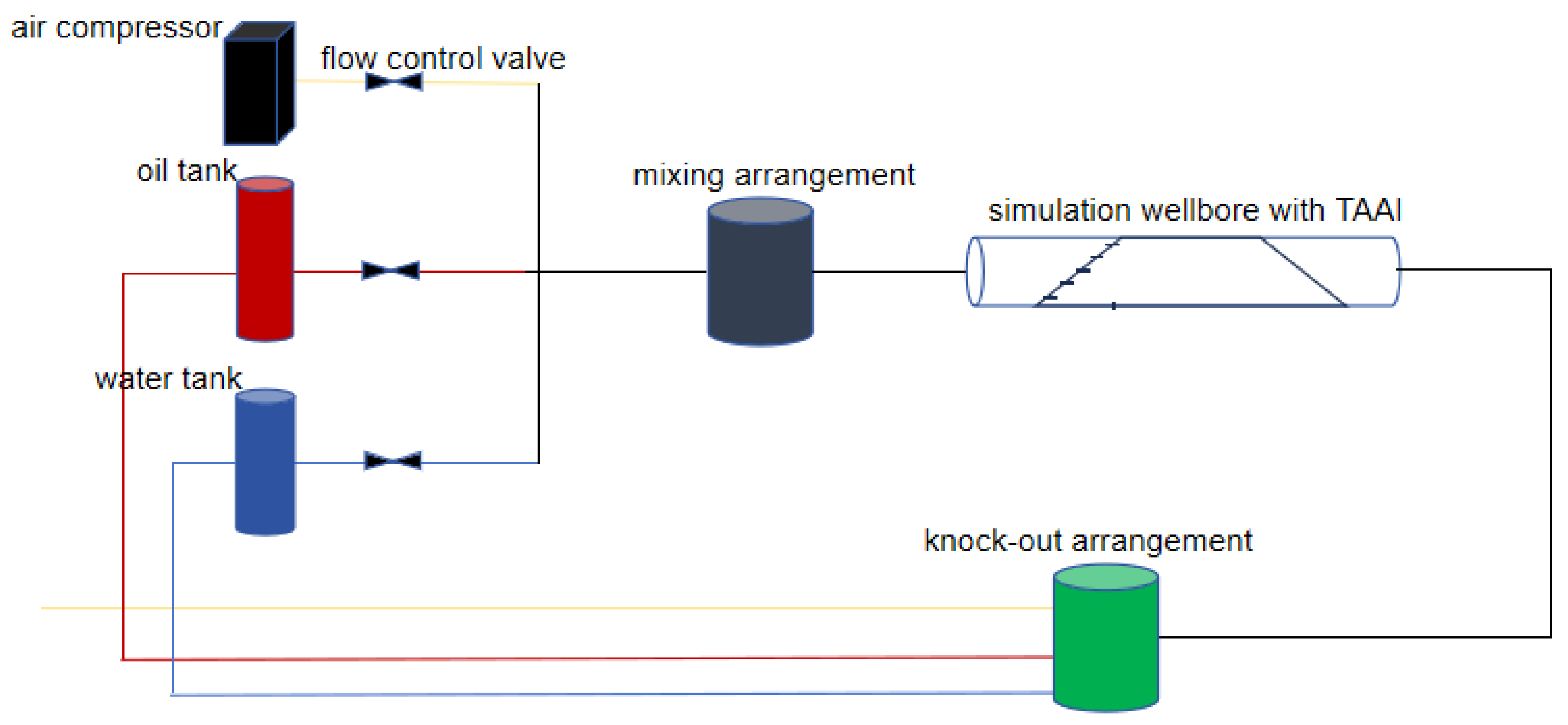
2.1. Simulation Experiments

The simulation experiments in this study were conducted using a flow loop simulation device, with the experimental data collected using a TAAI equipped with six fiber-optic probes. As shown in Figure 1.
To closely simulate downhole production conditions, the inner diameter of the experimental wellbore was set to 0.124 m, using air and tap water to represent natural gas and formation water, respectively. The experiments were conducted in one standard atmosphere pressure and a temperature of 30 °C. The density of air was tested to be 1.164 kg/m3 and the dynamic viscosity was 0.0187 mPa·s. The density of tap water was 995.7 kg/m3 and the dynamic viscosity was 0.7977 mPa·s. The experiment was designed with four different wellbore inclinations: 83°, 85°, 88°, and 90° (completely horizontal). The total gas–water flow rates of these four wellbore inclinations were 40, 60, 80, 100, 120, 140, and 160 m3/day. Their water cut conditions were 20%, 40%, 60%, and 80%.

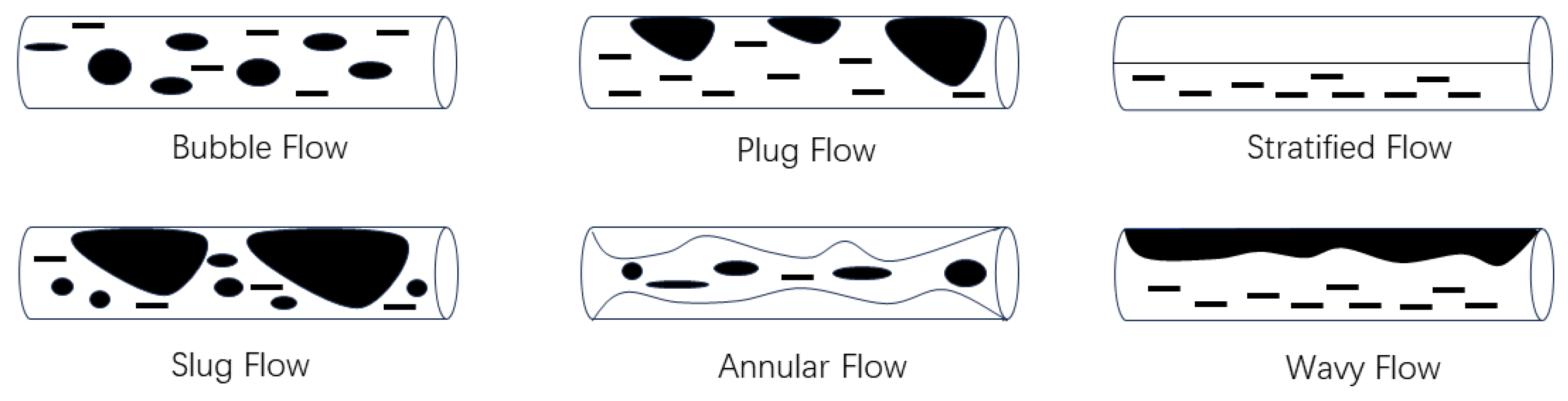
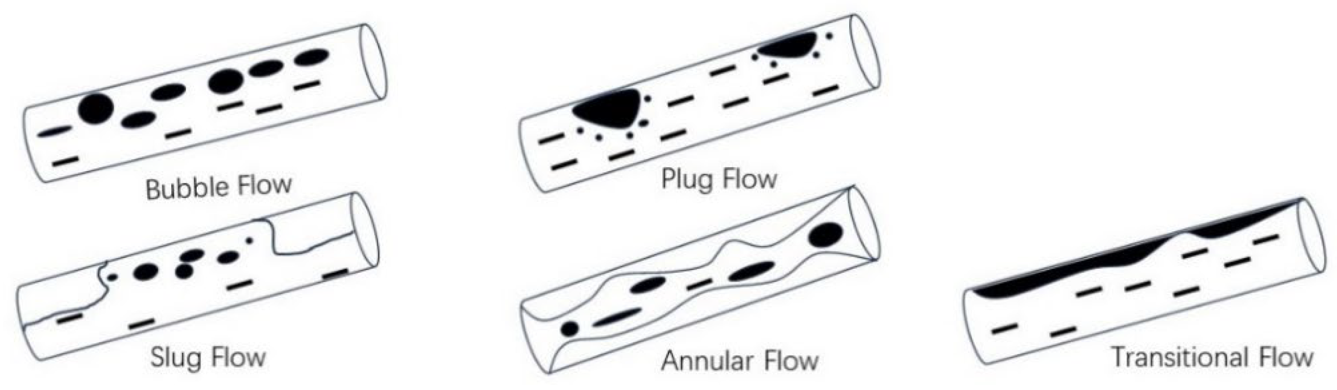
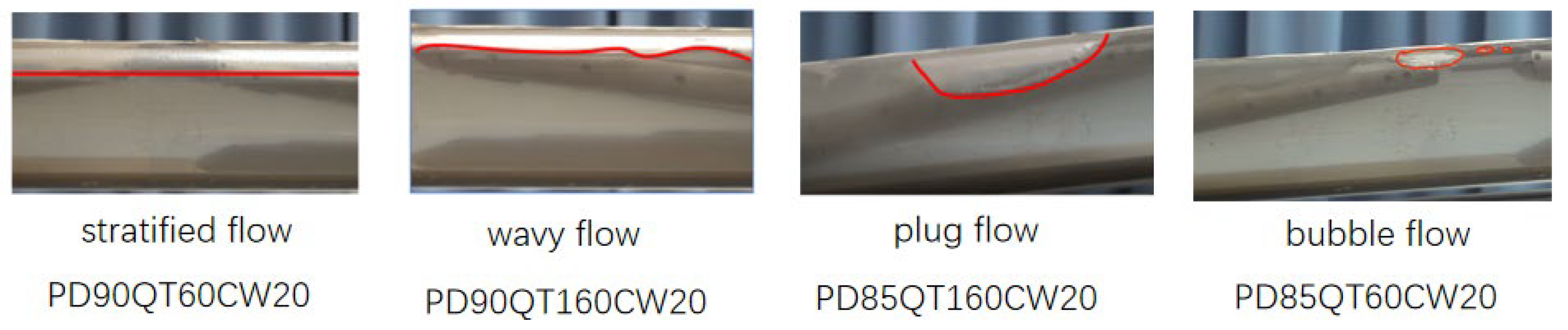
2.2. Flow Pattern Analysis

When two immiscible fluids flow within a wellbore, factors such as gravity and density differences cause the fluids to separate. In addition, variations in wellbore inclination and water cut result in these fluids flowing in different states and exhibiting distinct distribution characteristics known as flow patterns [14,15,16]. Under the influence of gravity, the distribution of liquid films and droplets within a horizontal wellbore tends to be non-uniform [15]. The gas–liquid two-phase flow in horizontal sections is asymmetrical, and numerous scholars and researchers categorize the gas–liquid flow patterns into four main types: stratified flow, intermittent flow, annular flow, and bubble flow. As shown in Figure 2, the flow pattern of gas and liquid in a horizontal wellbore can be primarily divided into six types: bubble flow, slug flow, stratified flow, wavy flow, plug flow, and annular flow. This classification has been widely recognized by international researchers [17,18,19,20].
As shown in Figure 3, when gas and liquid flow in an upward-inclined wellbore, variations in the wellbore inclination significantly impact the gas–liquid two-phase flow patterns. In this scenario, the flow patterns are primarily divided into five types: bubble flow, slug flow, plug flow, transitional flow, and annular flow [21].
As shown in Figure 4 and based on the aforementioned flow pattern classification combined with the specific conditions of these experiments, it was found that, at a horizontal inclination of 90°, the gas–water two-phase flow patterns are predominantly a stratified flow and wavy flow [22]. For an upward flow with an inclination less than 90°, the flow patterns are primarily a plug flow and bubble flow. From Figure 3, it can be observed that, with the same total flow rate and water cut, changes in the wellbore inclination result in fundamental changes in the gas–water two-phase flow patterns. Similarly, with the same wellbore inclination and water cut, changes in the total flow rate also lead to variations in the gas–water two-phase flow patterns.
Figure 5 presents the flow patterns observed from the simulation experiments in this study. In this figure, the X-axis represents the wellbore inclination in degrees (°); the Y-axis indicates water cut in percentage (%); and the Z-axis denotes the total flow rate in cubic meters per day (m3/day). The analysis reveals that, at a horizontal inclination of 90°, the predominant flow patterns are a stratified flow and wavy flow. As the total flow rate increases, the flow pattern transitions from a stratified flow to wavy flow. At inclinations of 83°, 85°, and 88°, the flow patterns are a plug flow and bubble flow.

3. Water Holdup Calculation

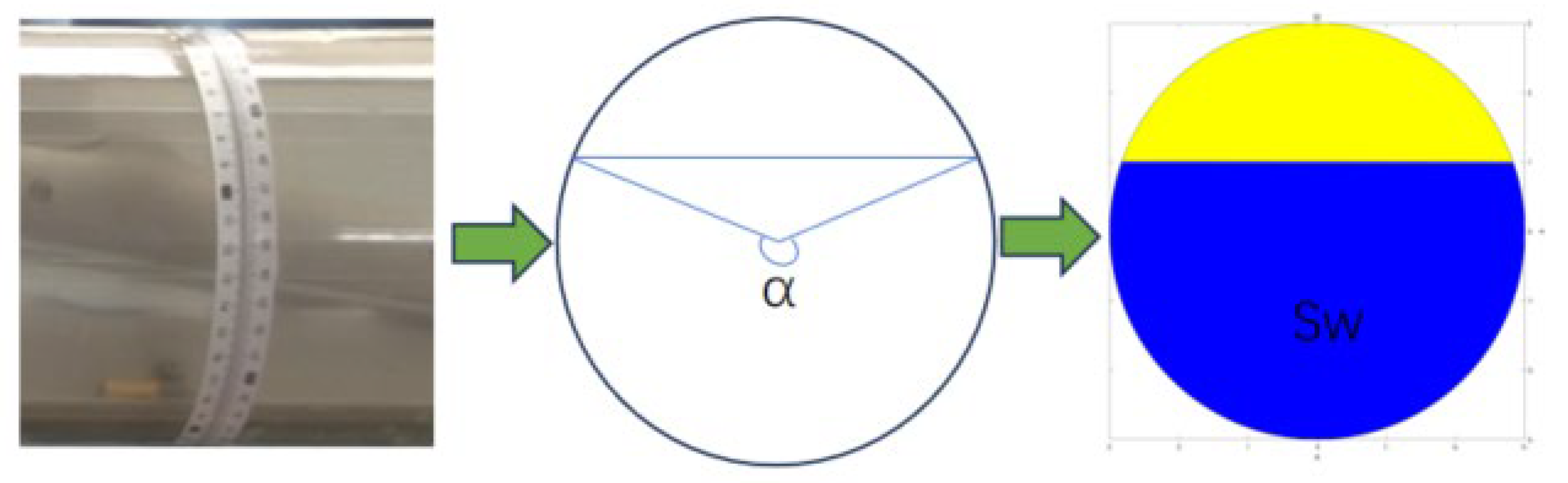
3.1. Calculation of Actual Water Holdup

Through the transparent simulation wellbore used in the experiments, the flow patterns and the phase interfaces between different fluids can be visually observed. A measuring scale wrapped around the wellbore allows for the reading of the liquid interface on the scale, from which the arc length, L, of the liquid surface can be obtained, enabling the calculation of the actual water holdup in the experiments [23]. As illustrated in Figure 6, the specific calculation process is as follows: knowing the arc length, L, of the liquid surface, the corresponding central angle, α, can be calculated. The area occupied by the water phase S w is then determined. The actual water holdup, Y ¯ w , is obtained by dividing the area of the water phase by the cross-sectional area of the wellbore, S a .
Y ¯ w = S w S a
where Y ¯ w represents the actual average water holdup in the wellbore cross-section; S a is the area of the wellbore cross-section; and S w indicates the area occupied by the water phase within the wellbore cross-section.

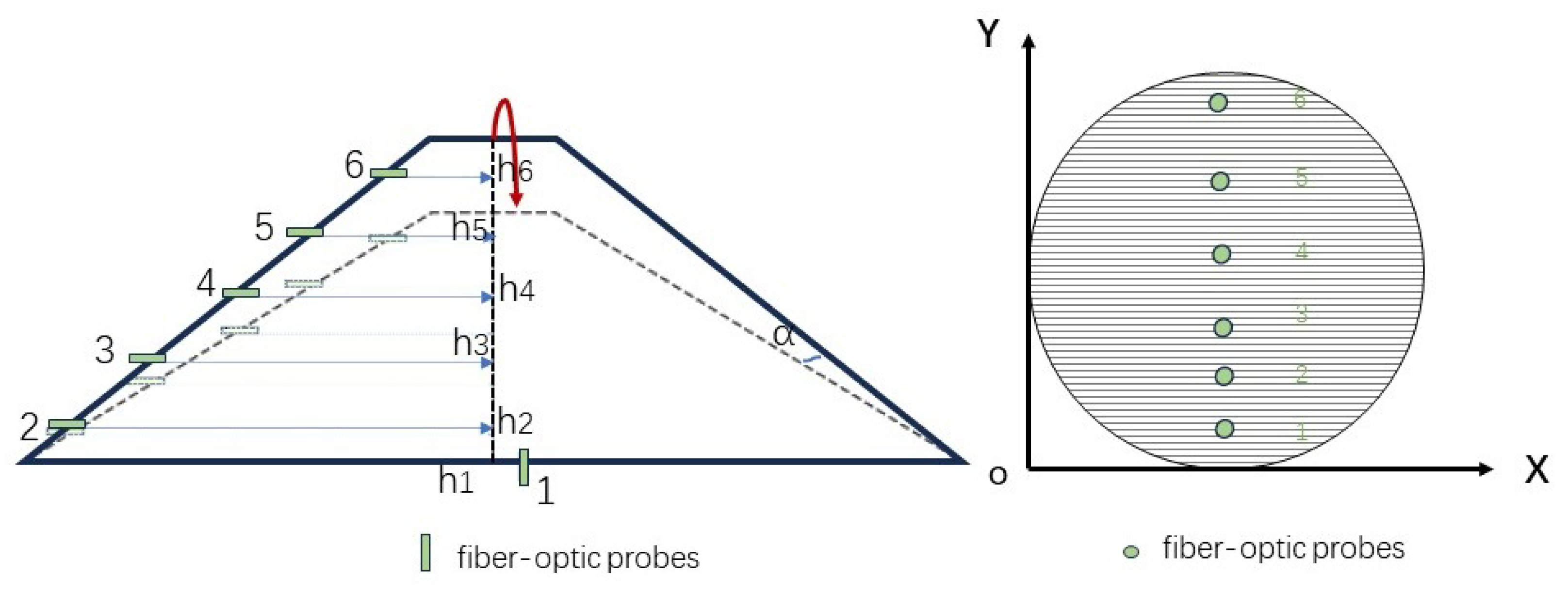
3.2. Calculation of Local Water Holdup Using Probes

Based on the calibration values of each fiber-optic probe for the water phase and gas phase, the local water holdup near the corresponding positions of each fiber-optic probe can be calculated using the following equation [19]:
Y w i = 1 A R M i A R M w A R M g A R M w
where Y w i is the local water holdup value of the ith fiber-optic probe; A R M w represents the response value of the ith fiber-optic probe; A R M g indicates the response value of the ith fiber-optic probe in pure gas; and A R M w indicates the response value of the ith fiber-optic probe in pure water.

3.3. Calculation of Probe Positions

When the wellbore inclination, gas–water flow rate, and water cut are constant, the fiber-optic probes positioned at different heights measure different fluid types, resulting in varying response values. As shown in Figure 7, when the TAAI instrument is conducting logging operations, it deflects to the left or right in the wellbore due to the dragging of the cable. The heights of the various probes on the wellbore cross-section are not constant. In this paper, based on the recorded rotation angle of the TAAI instrument, the TAAI instrument is repositioned to the midline of the wellbore cross-section. This allows for the precise calculation of the normalized heights of the six fiber-optic probes in the vertical direction of the wellbore cross-section.
h 1 = H 1 × ( cos α ) 2 C A L ( i = 1 )
h i = H 1 + L i × ( cos α ) 2 C A L ( i = 2 ,   3 , 4 , 5 )
h 6 = ( H 1 + L i + H 2 ) × ( cos α ) 2 C A L ( i = 6 )
where H 1 and H 2 are the thicknesses of the bottom and top of the instrument, respectively; h ( i = 1, 2, 3, 4, 5, 6) represents the normalized heights of each fiber-optic probe in the vertical direction of the wellbore cross-section; α denotes the rotation angle of the instrument; L i is the distance from the ith probe to the bottom end of the triangular arm; and C A L  is the wellbore diameter recorded by the instrument.

3.4. Segmentation of Wellbore Cross-Section

To calculate the water holdup in the wellbore cross-section and reduce calculation errors, this study used a weighted integration method instead of the traditional trapezoidal rule. As shown in Figure 7, the entire wellbore is horizontally segmented into n parts. The proportion of each segment relative to the entire circular wellbore cross-section ( P i ) , which serves as the weighting factor, was then determined. This proportion was used in subsequent calculations of the average water holdup of the wellbore cross-section by performing a weighted integration with the local water holdup values, thereby enhancing the accuracy of the water holdup calculation.
α i = Π 2 × a r c s i n x i r
x i = r i × n 2 r
S i = α i 2 × r 2 2 × x i 2 × tan α i + n 2 r 2 α i + n 2 r 2 × r 2 + 2 × x i + n 2 r 2 × tan α i + n 2 r 2
P i = S i Π × r 2
where r is the radius of the wellbore; x i represents the distance of the ith segment from the center of the circle; α i d enotes the central angle corresponding to the ith segment; S i is the area of the ith segment; and P i indicates the proportion of the ith segment relative to the entire wellbore cross-sectional area.

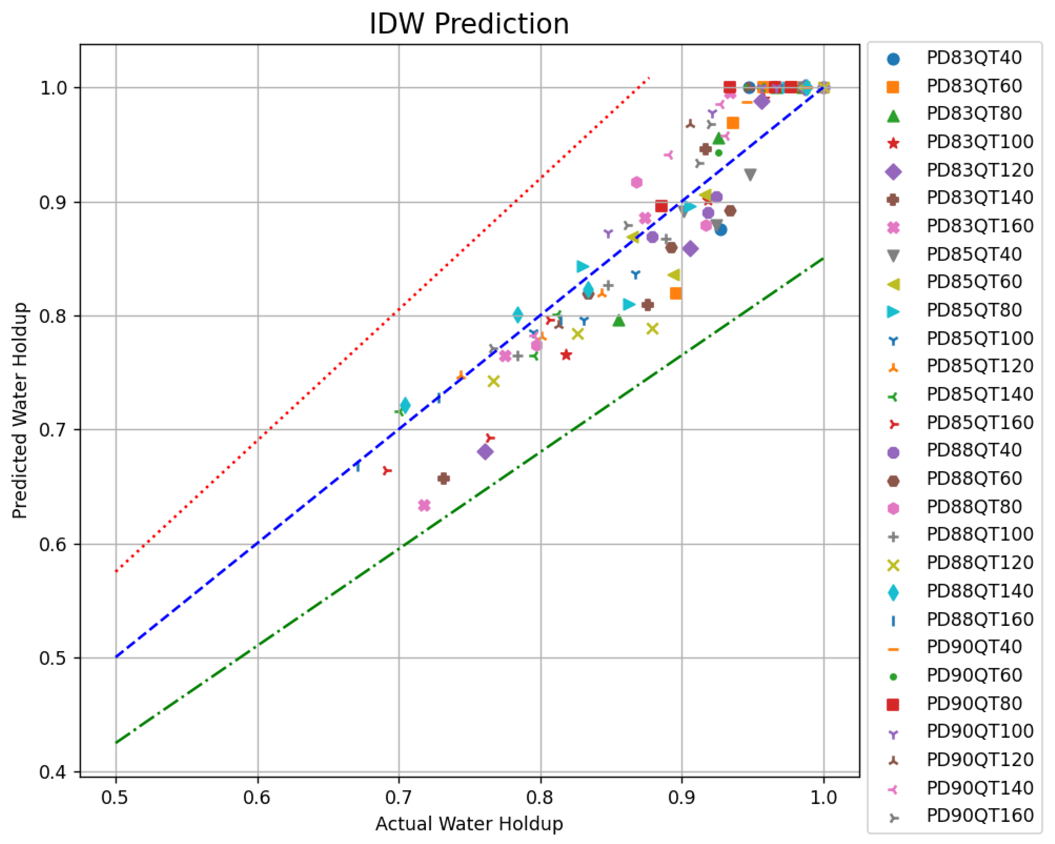
3.5. Comparison of GRBF and IDW Interpolation Algorithms

Based on the response values measured at the positions of the fiber-optic probes, both the GRBF and IDW interpolation methods were used to predict the local water holdup at unmeasured positions, thereby obtaining the average water holdup across the wellbore cross-section [24,25,26]. The differences between these two interpolation algorithms are shown in Table 1.
Clearly, different interpolation methods result in different predictions of local water holdup values at unmeasured positions. By performing the weighted integration of the local water holdup at different positions, the average water holdup Y w a G R B F and Y w a I D W at the current depth of the wellbore cross-section can be obtained.
Y w a G R B F = 1 n Y G R B F w i × P i
  Y w a I D W = 1 n Y i d w w i × P i
where Y w a G R B F represents the average water holdup at unmeasured positions calculated using the GRBF; Y G R B F w i is the local water holdup at the ith point interpolated using the GRBF; P i denotes the area proportion of the ith segment in the cross-section; Y w a I D W represents the average water holdup at unmeasured positions calculated using the IDW algorithm; and Y i d w w i indicates the local water holdup at the ith point interpolated using the IDW algorithm.
For gas–water two-phase experimental data with different wellbore inclinations, flow rates, and water cuts, the average water holdup in the wellbore cross-section was calculated using the two interpolation algorithms mentioned above. The results obtained by both methods were compared with the experimental shut-in water holdup, and their relative errors were analyzed. As shown in Figure 8 and Figure 9, the horizontal axis represents the shut-in water holdup and the vertical axis denotes the predicted water holdup. In the legends, PD represents wellbore inclination and QT indicates the total flow rate. The blue dashed line (y = x) indicates where the shut-in water holdup equals the predicted water holdup. The red dashed line represents a 15% upper relative error threshold and the green dashed line indicates a 15% lower relative error threshold. Compared to the shut-in water holdup, the maximum error for the water holdup calculated using the IDW algorithm was 15%, while the maximum error for the water holdup calculated using the GRBF method was 14%.
Clearly, the errors in the water holdup calculations using both the IDW and GRBF algorithms were relatively large, with both exceeding 10% when compared to the shut-in water holdup. Therefore, it is urgent to carry out optimization research to reduce the calculation error of the water holdup.

3.6. Principle of the L-M Algorithm

This study investigates relevant optimization algorithms to enhance the aforementioned two interpolation methods. Through comprehensive research, the following findings are summarized:
The Levenberg–Marquardt optimization algorithm (L-M) is an iterative optimization method designed for nonlinear minimization. It synergizes the advantages of the gradient descent method and Newton’s method by introducing a damping factor to balance their contributions, thereby adopting distinct optimization strategies at different stages. As a trust-region method, the L-M algorithm attempts a parameter update in each iteration and evaluates its acceptance based on whether the update reduces the error. If the update decreases the error, it is accepted, and the damping factor is reduced; otherwise, the update is rejected and the damping factor is increased. This mechanism effectively addresses redundant parameter issues and significantly reduces the likelihood of the cost function becoming trapped in local minima. These features are particularly critical for improving the inverse distance weighting (IDW) and generalized radial basis function (GRBF) interpolation algorithms, as they inherently face challenges related to parameter sensitivity and convergence stability [27,28].
The L-M algorithm is an iterative optimization algorithm used for nonlinear minimization. In this study, the L-M algorithm was utilized to iteratively optimize the GRBF and IDW interpolation algorithms. The process is as follows:
(1) Define the interpolation model: The model’s prediction result is:
Y i α , θ , λ = α × Y G R B F w i ( θ ) + 1 α × Y i d w w i ( λ )  
where Y i α , θ , λ is the predicted value given by the interpolation model; θ and λ are parameter vectors; α denotes the weighting parameter; Y G R B F w i indicates the local water holdup at the ith point interpolated using GRBF; and Y i d w w i represents the local water holdup at the ith point interpolated using the IDW algorithm.
(2) Define the residual vector: The residual vector   r i is composed of the differences between the observed values and the model predictions for each data point, as follows:
  r i = M i Y α , θ , λ
where  r i is the residual vector under the current parameters θ and  λ ; Mi denotes the actual measured original data; and Y α , θ , λ is the predicted value provided by the interpolation model.
(3) Define the objective function: The objective function, which is the sum of the squares of the residual vector, is used to minimize the residuals. The equation is as follows:
T α , θ , λ = i r i 2
where r i is the residual vector under the current parameters θ and λ .
(4) Mathematical derivation: The Jacobian matrix is defined as:
J α , θ , λ = T α T θ T λ
T α = 2 i = 1 ( Y i M i ) ( Y G R B F w i ( θ ) Y i d w w i ( λ ) )
T θ = 2 i = 1 ( Y i M i ) α Y G R B F w i θ
T λ = 2 i = 1 ( Y i M i ) ( 1 α ) Y i d w w i λ
(5) Introduce a regularization term: To prevent overfitting, a regularization term can be added to the objective function. The final objective function becomes:
  T r e g u l a r i z e d α , θ , λ = T α , θ , λ + δ α , θ , λ 2
where δ is the regularization parameter; θ , λ 2 represents the squared L2 norm of the parameter vectors.
(6) Minimizing the objective function: The L-M algorithm is used to minimize the regularized objective function,   T r e g u l a r i z e d α , θ , λ . By solving this optimization problem, the optimal parameters α , θ and λ are obtained, thereby improving the accuracy of the water holdup calculations from the two interpolation algorithms (GRBF and IDW).
In the LM optimization algorithm, the parameters include α , θ and λ . α controls the weight allocation between the IDW and GRBF interpolation methods, determining the model’s reliance on local features (IDW) versus global smoothness (GRBF). When α approaches 0, the model is dominated by the IDW algorithm, emphasizing the influence of local data points. When α approaches 1, the model is dominated by the GRBF, prioritizing global smoothness. θ (GRBF parameter) governs the smoothing range of the basic functions in the GRBF interpolation, determining the global fitting capability of the interpolated results. λ (IDW parameter) adjusts the decay rate of neighboring point weights with distance in the IDW interpolation, influencing the local sensitivity of the interpolated results. This parameterization allows the LM algorithm to adaptively balance local detail preservation and global trend representation during optimization.

4. Analysis of Optimization Results with the L-M Algorithm

The L-M algorithm was applied to the data processed using the IDW and GRBF methods as described earlier. The optimized results are shown in Figure 10.
In this figure, the horizontal axis represents the shut-in water holdup and the vertical axis denotes the predicted water holdup using three different algorithms. The legend indicates PD (wellbore inclination) and QT (total flow rate). The blue dashed line (y = x) indicates the situation where the predicted water holdup equals the shut-in water holdup. The red dashed line indicates a 15% upper relative error threshold and the green dashed line indicates a 15% lower relative error threshold. From Figure 10, it can be observed that the error in the water holdup calculated using the L-M algorithm is reduced to within 10%. In addition, the water holdup values predicted by the L-M algorithm are closer to the y = x baseline, indicating that the interpolation results have smaller errors, and the accuracy of the water holdup calculation is significantly improved.
Table 2, Table 3, Table 4 and Table 5 shows the results of the average water holdup and the real water holdup calculated by some experimental data. It can be seen that the error of the water holdup calculated by the L-M optimization algorithm is reduced to less than 10%.
It is important to note that under high water cut conditions in the gas–water two-phase experiments, as shown in Figure 8, Figure 9 and Figure 10 and the Table 2, Table 3, Table 4 and Table 5, the L-M algorithm could not effectively optimize the IDW and GRBF methods. This is because, at a high water cut, there was only a thin layer of gas at the top of the wellbore. The probes were still vertically distributed along the wellbore, but due to the design of the instrument, the topmost fiber-optic probe could not measure close to the top of the wellbore. Consequently, all the fiber-optic probes remained submerged in water and failed to detect the presence of gas. This limitation renders the L-M algorithm unsuitable for these extreme conditions.

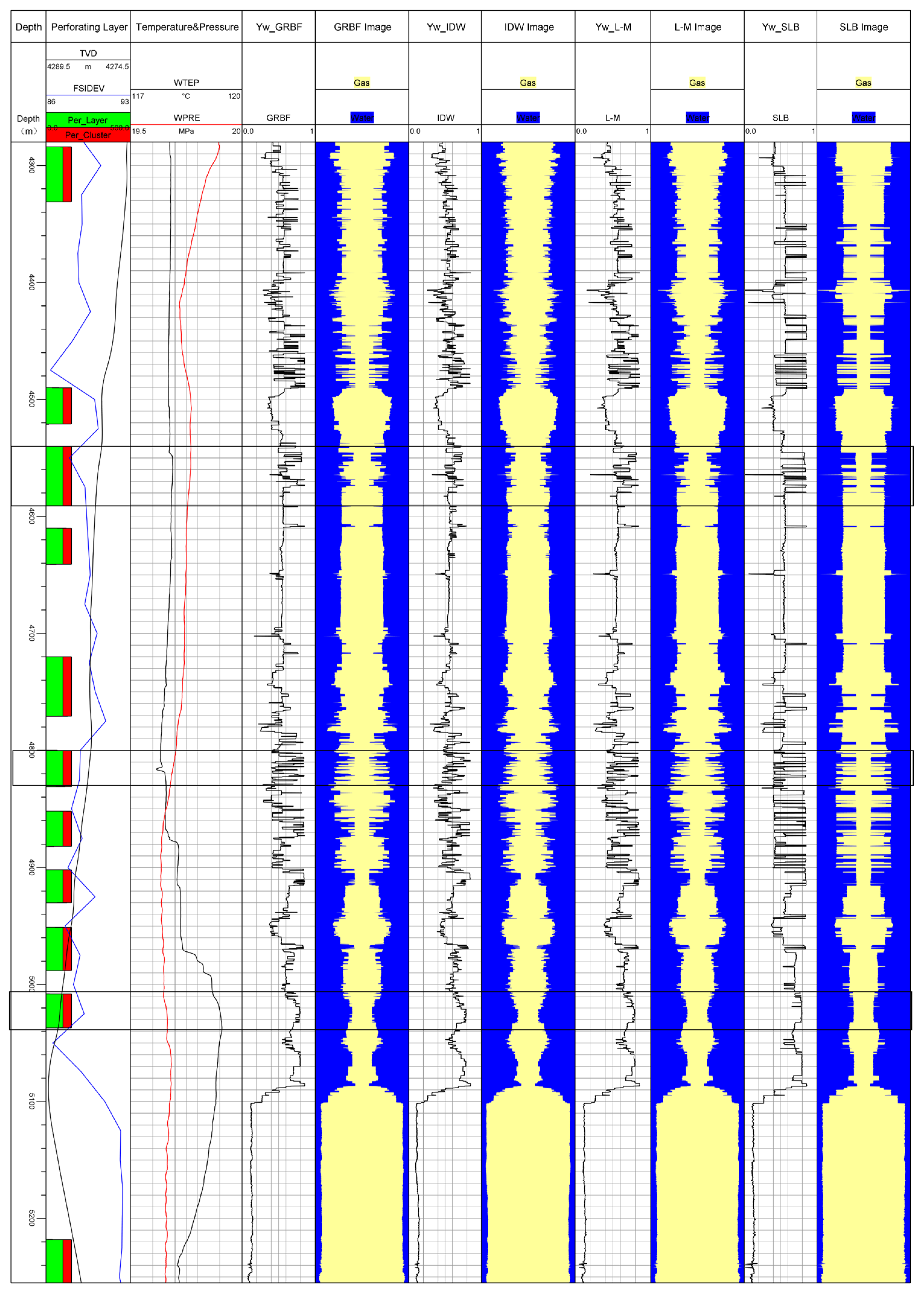
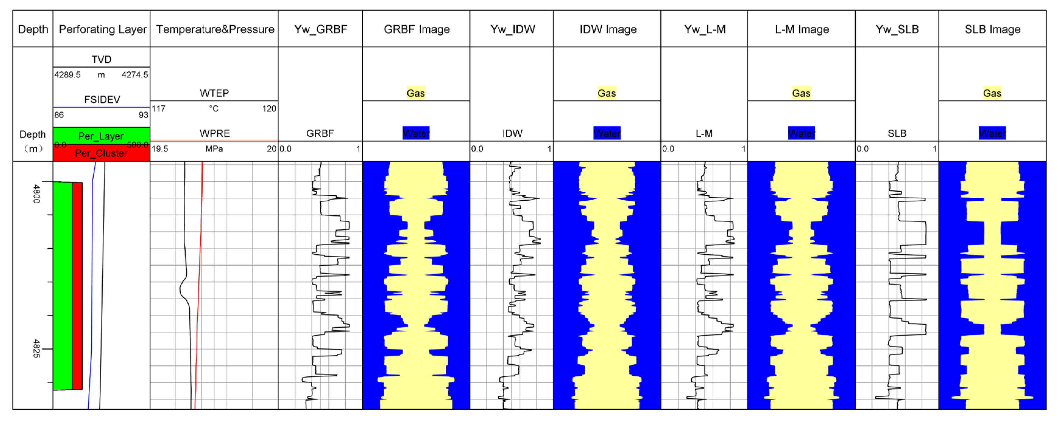
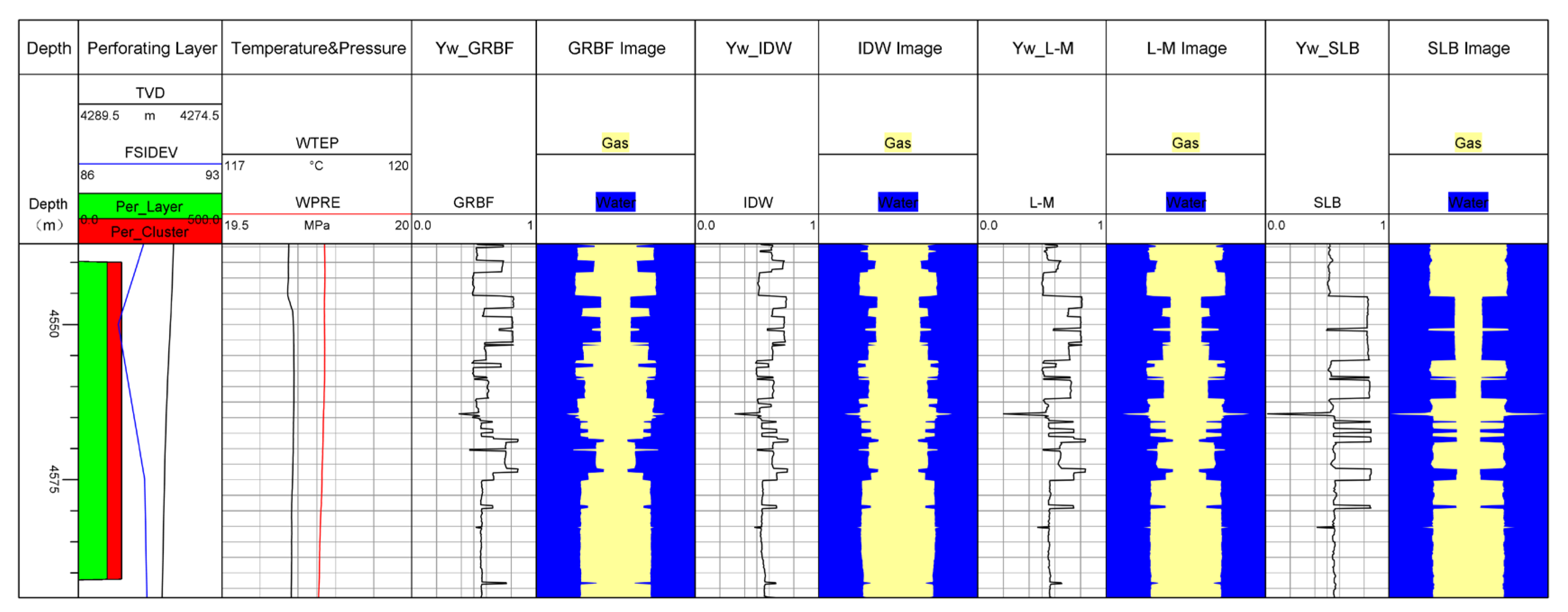
5. Case Study and Analysis

Well A is a gas–water two-phase horizontal well, with its horizontal section having 11 perforation layers. Its vertical depth ranges from 4200 m to 4214 m, and the measured slant depth ranges from 4282 m to 5294 m. The well inclination varies between 86° and 93°. The fluid from each perforation layer flows along the wellbore from right to left, with the wellbore experiencing horizontal, uphill, and downhill states.
As shown in Figure 11, from left to right, the columns represent the depth track, perforation layer, well inclination curve, vertical depth curve, temperature curve, pressure curve, GRBF water holdup curve, GRBF imaging, IDW water holdup curve, IDW imaging, L-M water holdup curve, L-M imaging, Schlumberger (SLB) water holdup curve, and SLB imaging. From the bottom to top, the rows represent production layers 1 to 11. Using the SLB water holdup curve as the benchmark, the accuracy of the three calculation methods (GRBF, IDW, and L-M) was compared for three different production layers, specifically layers 2, 6, and 9.
Layer 2 is a primary water-producing layer, which produces only water and no gas. The wellbore is in an uphill state, with the perforation depth ranging from 5008 m to 5037 m. The water holdup obtained by the three calculation methods is compared, as shown in Figure 12. From the vertical depth curve and well inclination curve, it can be seen that there is a downhill flow segment between the first and second layers. Due to the effect of gravity, the heavier water phase flows faster, while the lighter gas phase flows slower, leading to gas retention. As a result, there is a significant amount of gas between the first and second layers. In the second layer, which is uphill, the water (heavier phase) flows slower, and the gas (lighter phase) flows faster. Consequently, the fiber-optic probe detects the presence of gas in the second layer. However, because the water holdup curve does not change significantly, it is concluded that this layer does not produce gas, only water. Therefore, subsequent operations will focus on sealing this production section.
Layer 6 is a gas–water co-producing layer, primarily producing gas with a smaller amount of water. The wellbore is in an almost horizontal state, with a perforation depth ranging from 4800 m to 4831 m. The water holdup obtained by the three calculation methods is compared, as shown in Figure 13. From this figure, it can be seen that the water holdup curve shows significant fluctuations, indicating gas production from this layer. The wellbore cross-section contains more gas and less water, thus confirming that this layer predominantly produces gas with a small amount of water.
Layer 9 is a gas–water-producing layer, primarily producing water with a small amount of gas. The wellbore is in an uphill state, with a perforation depth ranging from 4540 m to 4591 m. The water holdup obtained by the three calculation methods is compared, as shown in Figure 14. From this figure, it can be seen that the water holdup curve shows variations, indicating gas production from this layer. The wellbore cross-section contains more water and less gas, confirming that this layer predominantly produces water with a small amount of gas.
As can be seen from Figure 12, Figure 13 and Figure 14 and Table 6, although the water holdup curve calculated by the three algorithms is generally consistent with the change trend of the water holdup explained by the third party, there is still a large error, and the calculation error of the GRBF and IDW algorithms is above 10%. Compared with the experiments conducted in this paper, by applying the IDW and GRBF interpolation algorithms to the actual production process, we can find that the relative error of calculating water holdup is larger.

6. Conclusion and Recommendations

(1) This study employed a flow loop simulation device and a TAAI to conduct gas–water two-phase simulation experiments under various wellbore inclinations, flow rates, and water cut conditions. The analysis reveals that, at a horizontal inclination of 90°, the predominant flow patterns are a stratified flow and wavy flow. At inclinations of 83°, 85°, and 88°, the flow patterns are a plug flow and bubble flow.
(2) Based on the processing and analysis of the experimental data, it can be concluded that, for well inclinations that are not perfectly horizontal (90°), the L-M optimization of the GRBF and IDW algorithms improves the accuracy by 4–5%, making the calculated average water holdup more consistent with the actual conditions.
(3) In the validation with case wells, Well A includes uphill, downhill, and horizontal states. In the horizontal state, the water holdup curves calculated by all three algorithms align with the third-party calculated water holdup. In the uphill and downhill states, the water holdup calculated using the L-M algorithm aligns more closely with the third-party calculated water holdup than the other two algorithms, thus improving the accuracy of the water holdup calculation.
(4) It is suggested to improve the TAAI so that the fiber-optic probes can get closer to the top of the wellbore, thus reducing the measurement blind spots of the instrument.

Author Contributions

Data curation: Y.C., J.L., F.G., X.Y. and B.Z.; writing—original draft preparation: Y.C.; writing—review and editing: Y.C. and J.L. All authors have read and agreed to the published version of the manuscript.

Funding

This paper is supported by the National Natural Science Foundation of China (No.42174163), Open Fund of Key Laboratory of Exploration Technologies for Oil and Gas Resources (Yangtze University), and Ministry of Education (Grant No. K2018-10).

Data Availability Statement

The data presented in this study are available on request from the corresponding author.

Conflicts of Interest

Authors Feng Gao, Xiaotao Yuan and Boxin Zhang were employed by the Xinjiang Branch, China National Logging Corporation. The remaining authors declare that the research was conducted in the absence of any commercial or financial relationships that could be construed as a potential conflict of interest.

References

  1. Cui, S.F. Research on Simulation Experiment and Interpretation Method of Horizontal Well Array Flow Imager. Master’s Thesis, Yangtze University, Jingzhou, China, 2022. [Google Scholar]
  2. Chen, H.; Sun, W.; Zou, S. Applied Study of Three-Phase Flow Production Profile Testing Technology with FAST Array Tools. J. Jianghan Pet. Univ. Staff. Work. 2024, 37, 23–25, 32. [Google Scholar]
  3. Wang, T.; Liu, J.; Li, B.; Deng, H.; Cui, S. Analysis of gas-water two-phase holdup of horizontal well based on array fiber probe. Yunnan Chem. Technol. 2020, 47, 60–61. [Google Scholar]
  4. Mu, H.; Liu, W.; Kong, L.; Li, Y.; Liu, C.; Liu, X. Experimental study on the response characteristics to the optical fiber gas holdup in the gas/water two-phase flow. Opt. Instrum. 2012, 34, 66–69. [Google Scholar]
  5. Yang, R.; Liu, J.; Li, M.; Cui, S.; Hu, H.; Li, Y. Simulation Experiment and Interpretation Research of Gas-Water Two-Phase Horizontal Well Array Imager. Available online: http://kns.cnki.net/kcms/detail/11.2982.p.20241205.1223.073.html (accessed on 16 January 2025).
  6. Li, A.; Guo, H.; Niu, Y.; Lu, X.; Zhang, Y.; Liang, H.; Sun, Y.; Guo, Y.; Wang, D. Application of Imaging Algorithms for Gas–Water Two-Phase Array Fiber Holdup Meters in Horizontal Wells. Sensors 2024, 24, 7285. [Google Scholar] [CrossRef] [PubMed]
  7. Hu, S.L. Application of gas array tool in monitoring gas production profile of highly-deviated wells. Oil Gas Well Detect. 2024, 33, 56–60. [Google Scholar]
  8. Xing, W.; Chen, Q.; Liu, G. Gas-holding rate imaging method for gas-liquid two-phase flow based on single-mode fiber probe. Opt. Commun. Technol. 2025, 49, 78–82. [Google Scholar]
  9. Song, W.R.; Li, W.H.; Lin, S.Y.; Ye, H.R.; Li, G. Experimental and numerical investigation of flow pattern evolution and flow-induced vibrations in an M-shaped subsea jumper under gas-liquid two-phase flow conditions. Ocean. Eng. 2025, 327, 120964. [Google Scholar] [CrossRef]
  10. Muhammad Waqas, Y.; Ramasamy, M.; Risza, R.; Reddy Prasad, D.M.; Rajashekhar, P. Review on gas–liquid–liquid three–phase flow patterns, pressure drop, and liquid holdup in pipelines. Chem. Eng. Res. Des. 2020, 159, 505–528. [Google Scholar]
  11. Yan, P. Research on Measurement Method of Gas Holdup of Horizontal Gas-Liquid Two-Phase Flow Based on Array Optical Fiber Sensing. Master’s Thesis, Yanshan University, Qinhuangdao, China, 2023. [Google Scholar]
  12. Wu, Y. Measurement Method of Acoustic-Electric Sensors for Phase Holdup in Horizontal Gas-Liquid Two-Phase Flow. Ph.D. Thesis, Tianjin University, Tianjin, China, 2020. [Google Scholar]
  13. Kong, W.; Li, S.; Hao, H.; Yan, P.; Zhuo, C.; Li, H. Measurement method of gas holdup in horizontal gas-liquid two-phase flow based on fiber-optic probe array. Flow Meas. Instrum. 2024, 97, 102588. [Google Scholar] [CrossRef]
  14. Liu, J.; Jiang, L.; Chen, Y.; Liu, Z.; Yuan, H.; Wen, Y. Study on prediction model of liquid hold up based on random forest algorithm. Chem. Eng. Sci. 2023, 268, 118383. [Google Scholar] [CrossRef]
  15. Ma, T.; Wang, T.; Wang, L. A hybrid deep learning model towards flow pattern identification of gas-liquid two-phase flows in horizontal pipe. Energy 2025, 320, 135–141. [Google Scholar]
  16. Shi, Y.; Sun, Y.; Wang, M.; Zhang, S.; Yang, Z. Flow pattern recognition for horizontal gas-liquid two-phase flow with a hybrid deep-learning model. Flow Meas. Instrum. 2025, 102, 102829. [Google Scholar]
  17. Saisorn, S.; Benjawun, P.; Suriyawong, A.; Wongwises, S. Experimental investigation on flow pattern and void fraction for two-phase gas-liquid upflow in a vertical helically coiled micro-channel. Int. J. Thermofluids 2025, 26, 101124. [Google Scholar]
  18. Liu, D.W.; Yang, B.J.; Zhang, W.B.; Xue, X.B. Analysis of gas-liquid two-phase flow characteristics of wellbore in horizontal wells. China Pet. Chem. Stand. Qual. 2023, 43, 81–84. [Google Scholar]
  19. Chen, S.; Liu, S.; Liu, L.; Li, Y.; Zhang, J.; Cong, T.; Gu, H. Experimental study on flow patterns and pressure gradient of decaying swirling gas-liquid flow in a horizontal pipe. Prog. Nucl. Energy 2024, 177, 105445. [Google Scholar]
  20. Ma, H.; Xu, Y.; Huang, H.; Yuan, C.; Wang, J.; Yang, Y.; Wang, D. Intelligent predictions for flow pattern and phase fraction of a horizontal gas-liquid flow. Energy 2024, 303, 131944. [Google Scholar] [CrossRef]
  21. Zhang, X.; Hou, L.; Zhu, Z.; Liu, J.; Sun, X.; Hu, Z. Flow pattern identification of gas-liquid two-phase flow based on integrating mechanism analysis and data mining. Geoenergy Sci. Eng. 2023, 228, 212013. [Google Scholar]
  22. Liu, Y.; Luo, C.; Liu, T.; Ren, G.; Wang, Z. Prediction of Gas-liquid Two-phase Flow Patterns in Horizontal Gas Wells. J. Southwest Pet. Univ. 2019, 41, 107–112. [Google Scholar]
  23. Yang, Q.; Jin, N.; Wang, F.; Ren, W. Measurement of Gas Phase Distribution Using Multifiber Optical Probes in a Two-Phase Flow. IEEE Sens. J. 2020, 20, 6642–6651. [Google Scholar] [CrossRef]
  24. Karimi, N.; Kazem, S.; Ahmadian, D.; Adibi, H.; Ballestra, L.V. On a generalized Gaussian radial basis function: Analysis and applications. Eng. Anal. Bound. Elem. 2020, 112, 46–57. [Google Scholar] [CrossRef]
  25. Li, Z.; Zhang, X.; Zhu, R.; Zhang, Z.; Weng, Z. Integrating data-to-data correlation into inverse distance weighting. Comput. Geosci. 2020, 24, 203–216. [Google Scholar] [CrossRef]
  26. Jin, G.D.; Liu, Y.C.; Niu, W.J. Comparison between Inverse Distance Weighting Method and Kriging. J. Chang. Univ. Sci. Technol. 2003, 24, 53–57. [Google Scholar]
  27. de Jesús Rubio, J. Stability Analysis of the Modified Levenberg–Marquardt Algorithm for the Artificial Neural Network Training. IEEE Trans. Neural Netw. Learn. Syst. 2021, 32, 3510–3524. [Google Scholar] [CrossRef] [PubMed]
  28. Shaik, N.B.; Sayani, J.K.S.; Benjapolakul, W.; Asdornwised, W.; Chaitusaney, S. Experimental investigation and ANN modelling on CO2 hydrate kinetics in multiphase pipeline systems. Sci. Rep. 2022, 12, 13642. [Google Scholar] [CrossRef] [PubMed]
Figure 1. Schematic diagram of the simulated experimental setup.
Processes 13 01004 g001
Figure 2. Gas–liquid two-phase flow patterns in a horizontal wellbore.
Processes 13 01004 g002
Figure 3. Gas–liquid two-phase flow patterns in an upward-inclined wellbore.
Processes 13 01004 g003
Figure 4. Main flow patterns in the experiments. GW: gas–water two-phase flow; PD: wellbore inclination (°); QT: total flow rate (m3/day); CW: water cut (%).
Processes 13 01004 g004
Figure 5. Diagram of flow patterns observed in the experiments.
Processes 13 01004 g005
Figure 6. Schematic diagram for the calculation of actual water holdup.
Processes 13 01004 g006
Figure 7. Schematic diagram of instrument rotation and probe positions.
Processes 13 01004 g007
Figure 8. Calculation results of IDW.
Processes 13 01004 g008
Figure 9. Calculation results of the GRBF.
Processes 13 01004 g009
Figure 10. Optimization results of the L-M algorithm.
Processes 13 01004 g010
Figure 11. Comparison of water holdup curves.
Processes 13 01004 g011
Figure 12. Comparison of water holdup curves.
Processes 13 01004 g012
Figure 13. Comparison of water holdup curves.
Processes 13 01004 g013
Figure 14. Comparison of water holdup curves.
Processes 13 01004 g014
Table 1. Comparison of GRBF and IDW interpolation methods.
Feature GRBFIDW
Interpolation principleIt uses a Gaussian function to weight sample points and obtain the interpolated result through a weighted summation.It weights by the inverse of distance, adding more weight to nearer points.
Data requirementIt requires a sufficient number of sample points to fit the Gaussian function.It can achieve interpolation results with relatively fewer sample points.
SmoothnessIt provides smoothness and effectively suppresses noise.It is sensitive to noise and may be affected by local extreme values.
Data distributionIt has no special assumptions about data distribution.It works well with densely distributed data but may be less suitable for unevenly distributed data.
Parameter adjustmentIt requires adjusting parameters of the Gaussian function, needing some experience.It has only one parameter (power exponent), making it relatively easy to adjust.
Computational complexityIt involves calculations with Gaussian functions, leading to higher computational complexity.It is simple to compute and suitable for large-scale data interpolation.
Global and local characteristics of interpolation resultsIts results are local to some extent, focusing more on the influence of nearby sample points.Its results are global, with all sample points influencing the interpolation result equally.
Table 2. Comparison analysis table of average and true water holdup value in 83° parts of gas and water phases calculated by different algorithms.
Total Flow
(m3/d)
Water Holdup
(%)
Real Water HoldupIDW Water HoldupGRBF Water HoldupL-M
Water Holdup
IDW Relative Error (%)GRBF
Relative Error (%)
L-M
Relative Error (%)
40200.9270.8760.8960.9365.503.340.97
400.9471115.605.605.60
600.9861111.421.421.42
800.9931110.700.700.70
140200.7320.6570.6870.69710.26.154.78
400.8760.8090.9040.9047.653.203.20
600.9170.9460.9560.9363.164.252.07
800.9661113.523.523.52
160200.7180.6340.7340.73411.72.232.23
400.7750.7650.7850.7851.291.291.29
600.8740.7440.7860.78714.8710.079.95
800.9340.9960.9960.9966.646.646.64
Table 3. Comparison analysis table of average and true water holdup values in 85° parts of gas and water phases calculated by different algorithms.
Total Flow
(m3/d)
Water Holdup
(%)
Real Water HoldupIDW Water HoldupGRBF Water HoldupL-M
Water Holdup
IDW Relative Error (%)GRBF
Relative Error (%)
L-M
Relative Error (%)
40200.9010.8310.8590.9217.774.662.22
400.9240.8210.8390.86911.159.205.95
600.9481115.495.495.49
800.9861111.421.421.42
140200.7010.7160.6790.6892.143.141.71
400.7960.7650.8150.8153.892.392.39
600.8120.8010.7910.7911.352.592.59
800.9561114.604.604.60
160200.6910.6640.6440.6743.916.802.46
400.7640.7330.7830.7834.062.492.49
600.8060.7760.7860.7863.722.482.48
800.9471115.605.605.60
Table 4. Comparison analysis table of average and true water holdup values in 88° parts of gas and water phases calculated by different algorithms.
Total Flow
(m3/d)
Water Holdup
(%)
Real Water HoldupIDW Water HoldupGRBF Water HoldupL-M
Water Holdup
IDW Relative Error (%)GRBF
Relative Error (%)
L-M
Relative Error (%)
40200.8790.8690.8890.8861.141.140.80
400.9180.880.870.894.145.233.05
600.9240.9040.9740.9342.165.411.08
800.9391116.506.506.50
140200.7040.6790.7410.7213.555.262.41
400.7840.8010.8010.8012.172.172.17
600.8340.8230.8630.8631.323.483.48
800.9881111.211.211.21
160200.6710.6780.6780.6681.041.040.45
400.7280.6880.7580.7485.494.122.75
600.8140.7960.7960.7962.212.212.21
800.9671113.413.413.41
Table 5. Comparison analysis table of average and true water holdup values in 90° parts of gas and water phases calculated by different algorithms.
Total Flow
(m3/d)
Water Holdup
(%)
Real Water HoldupIDW Water HoldupGRBF Water HoldupL-M
Water Holdup
IDW Relative Error (%)GRBF
Relative Error (%)
L-M
Relative Error (%)
40200.8460.8660.8370.8562.361.061.18
400.8980.8750.9210.8822.562.561.78
600.9280.9080.9780.9182.165.391.08
800.9881111.211.211.21
800.9571114.494.494.49
140200.7360.7160.7570.7482.722.851.63
400.8510.8760.8340.8672.942.001.88
600.8910.9140.8620.9082.583.251.91
800.9501115.265.265.26
160200.6670.6880.6570.6753.151.501.20
400.7210.7040.7440.7092.363.191.66
600.8120.7860.8540.7993.205.171.60
800.9200.8960.9650.942.614.892.17
Table 6. Comparison table of relative error of typical yield water holdup of different algorithms.
LayerYw_SLBYw_GRBFYw_IDWYw_L-MGRBF Relative Error (%)IDW
Relative Error (%)
L-M
Relative Error (%)
20.7940.6940.7070.72412.6%11.08.8%
60.5790.5210.5180.53310.0%10.57.9%
90.7250.6480.6320.78910.6%12.88.1%
Disclaimer/Publisher’s Note: The statements, opinions and data contained in all publications are solely those of the individual author(s) and contributor(s) and not of MDPI and/or the editor(s). MDPI and/or the editor(s) disclaim responsibility for any injury to people or property resulting from any ideas, methods, instructions or products referred to in the content.

