Article

Dual-Branch Discriminative Transmission Line Bolt Image Classification Based on Contrastive Learning

1
State Grid Hebei Electric Power Research Institute, Shijiazhuang 050000, China
2
School of Mechanical Engineering, Sichuan University, Chengdu 610065, China
*
Author to whom correspondence should be addressed.
Processes 2025, 13(3), 898; https://doi.org/10.3390/pr13030898
Submission received: 26 December 2024 / Revised: 21 February 2025 / Accepted: 24 February 2025 / Published: 19 March 2025
(This article belongs to the Topic Advances in Power Science and Technology, 2nd Edition)

Abstract

:
The classification of transmission tower bolt images faces challenges such as class imbalance, sample scarcity, and the low pixel proportion of pins. Traditional classification methods exhibit poor performance in identifying key categories with small proportions, fail to leverage the correlation between transmission line fittings and bolts, and suffer from severe false positive issues. This study proposes a novel approach that dynamically integrates two sampling strategies to address the class imbalance problem while incorporating contrastive learning and category labels to enhance the discrimination of easily confused samples. Additionally, an auxiliary branch discrimination mechanism effectively exploits the correlation between fittings and bolts and, combined with a threshold-based decision process, significantly reduces the false positive rate (by 3.74%). The experimental results demonstrate that, compared to the baseline SimCLR framework with ResNet18, the proposed method improves accuracy (Acc) by 10.22%, reduces the false alarm rate by 5%, and significantly enhances classification reliability in transmission line inspections, thereby mitigating unnecessary human resource consumption.

1. Introduction

Bolts are indispensable components of transmission towers, essential for connecting tower body components and securing fittings to the tower. Some bolts require pins as mechanical locking mechanisms, and their detachment poses a threat to the structural integrity of the transmission tower. The pin-related properties of bolts are classified into three categories: Class 1 is BP (Bolt without Pin), which refers to bolts used for connecting tower body components that should not have pins; Class 2 is BWP (Bolt with Pin), which refers to bolts securing various fittings to the tower body, where pins should be present and properly retained; and Class 3 is BLP (Bolt Losing Pin), which represents defective cases of BWPs, where pins should be present but are missing.
In recent years, manual periodic inspections have been gradually replaced by aerial photography using unmanned aerial vehicles (UAVs). However, aerial survey images suffer from issues such as a limited sample size, severe class imbalance, and small target objects. Previous studies have attempted to simultaneously perform bolt localization and classification by directly adopting object detection networks that have demonstrated strong performance in other domains, including single-stage networks such as SSD [1] and YOLO [2], as well as two-stage networks such as Faster R-CNN [3] and Cascade R-CNN [4]. Taking Cascade R-CNN as an example, which achieves the best overall performance, prior research has shown that this network can effectively perform bolt localization (i.e., evaluating only the total number of correctly detected bolts without considering classification accuracy), achieving a localization accuracy exceeding 95%. However, its classification performance is relatively poor (i.e., evaluating the classification accuracy of correctly localized bolts). The original aerial survey image data rely on manual annotation, and the small sample size leads to suboptimal model performance. Among all categories, BLP has the smallest proportion, and the class imbalance issue results in poor classification performance for this critical category. Additionally, bolts occupy only a small portion of the original image, while pin-related information represents an even smaller proportion of the bolt, which may lead to the loss of critical information during downsampling. Therefore, independently training a bolt classification network at a higher resolution is both necessary and meaningful.
In image classification tasks, He et al. [5] were the first to propose a method in which a single image is randomly augmented (e.g., cropping, color perturbation, flipping, rotation, and scaling) to generate two transformed images, and contrastive learning is then applied to extract their shared features. In contrastive learning, this random augmentation strategy enhances data diversity and, to some extent, mitigates the small sample size issue. By integrating contrastive loss with category labels [6], this approach reduces intra-class variations among positive samples while increasing the differences between negative samples, thereby preventing the loss of critical information and improving the differentiation between BP and BLP.
To address the data imbalance problem, commonly used techniques include oversampling, undersampling, and reweighting methods [7]. Tsung et al. [8] proposed the Focal Loss function, which adjusts the loss weights of samples with varying classification difficulty to improve performance on hard-to-classify samples. While this method alleviates the data imbalance issue to some extent, it often fails to adapt dynamically to changes in sample difficulty during training, potentially leading to overfitting or insufficient focus on minority-class samples. In this study, UNIS (Uniform Sampling) and INVS (Inverse Sampling) are introduced to dynamically adjust their weights in the loss function, effectively addressing the class imbalance problem.
The presence of pins is closely related to transmission line fittings, yet previous studies have failed to effectively exploit this correlation. Feng et al. [9] proposed an auxiliary discrimination system based on an experience library, which has shown promising results in defect detection. Since the number of fitting types is limited, manually annotating and identifying each type would significantly increase workload. Instead, cluster analysis is employed to obtain category centers. If a pin is present, it must share similarities with the category center of a specific type of fitting. By incorporating a threshold-based decision mechanism for secondary discrimination, the probability of BP being misclassified as BLP is reduced.
The structure of this paper is as follows:
  • Section 1 introduces the background and research approach.
  • Section 2 describes the network architecture, the functionality of each module, and the design of the loss function.
  • Section 3 details the selection of hyperparameters and the design and results of comparative and ablation experiments.
  • Section 4 summarizes the contributions and conclusions of this study.
  • Section 5 discusses the limitations of the proposed model, its potential applications in other domains, and future research directions.

2. Materials and Methods

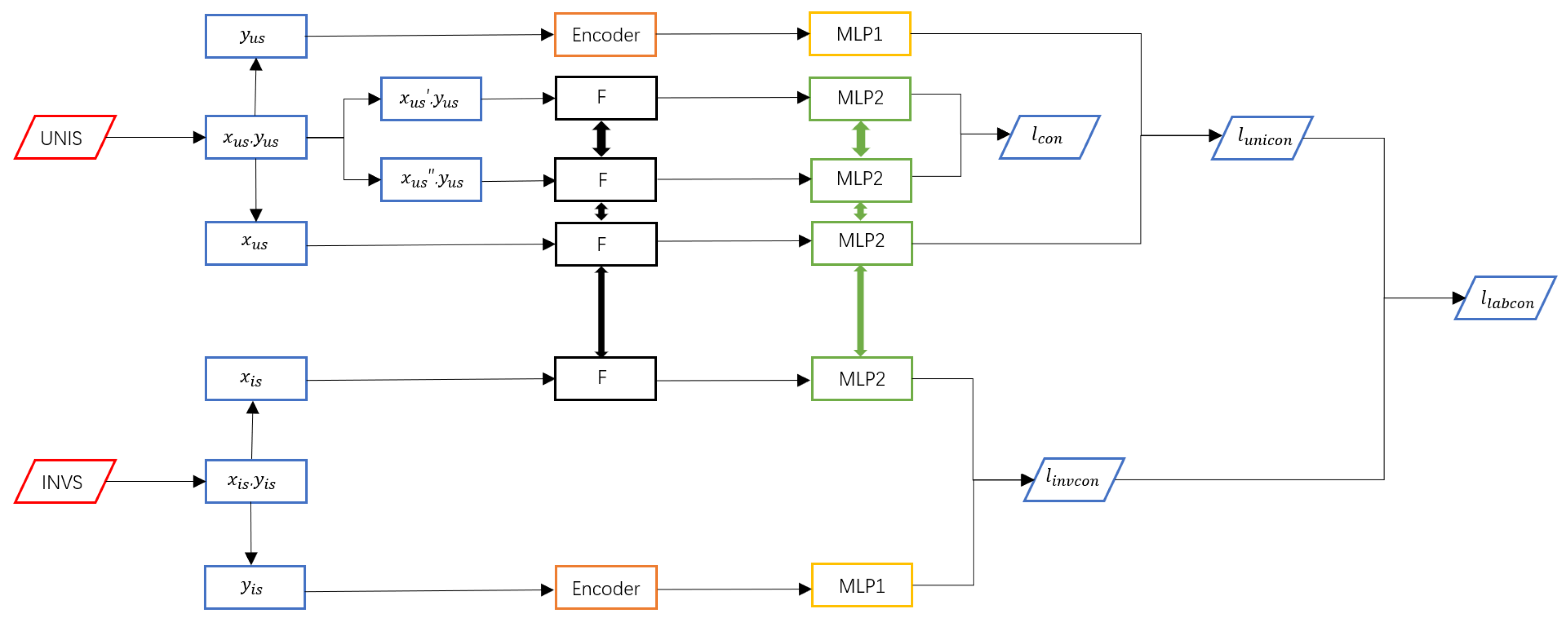
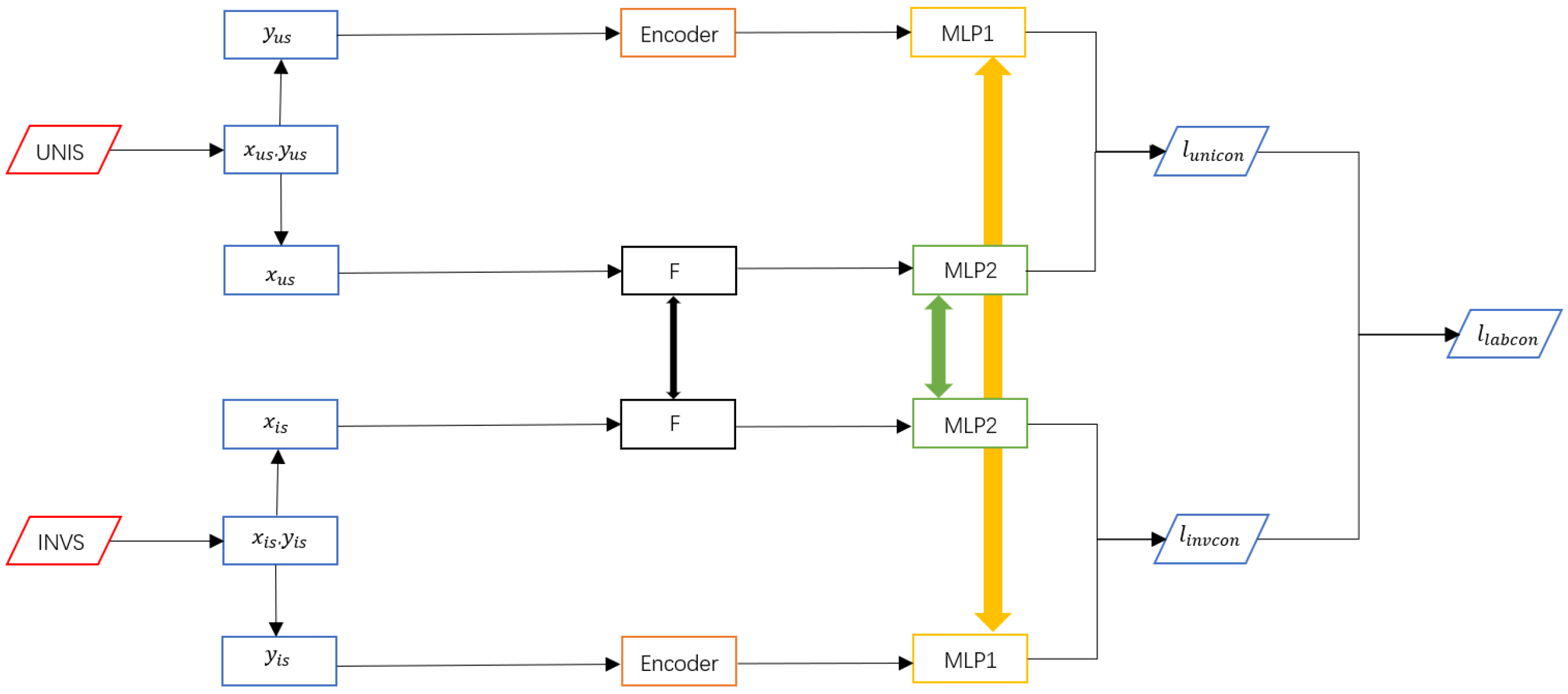
2.1. An Overview of the Training Phase

During the training phase, the network can be divided into three functional modules, as shown in Figure 1. UNIS and INVS are responsible for sample selection [10], with their weights being dynamically adjusted through adaptive weighting. F (feature extraction) handles feature extraction for all images. The contrastive learning module applies data augmentation to UNIS’s data before performing contrastive learning. In the category label module, the two modalities of information—image information ( x u s , x i s ) and label information ( y u s , y i s )—from both the UNIS and INVS are processed through different methods and then compared within the same feature space. The processing pipeline consists of five steps.
(1)
Input: The samples collected by UNIS contain two modalities: label information and image information. The images undergo random augmentation before being used for contrastive learning training. The labels and original images are fed into the image channel and label channel, respectively. INVS follows the same processing pipeline as UNIS, except that it does not perform random augmentation or contrastive learning.
(2)
Feature extraction: All F modules adopt the ResNet18 architecture with shared weights.
(3)
Contrastive learning: The samples collected by UNIS are augmented and then used for contrastive learning, where the similarity between positive sample pairs is maximized, and the differences between negative sample pairs are minimized.
(4)
Feature normalization: Both image and label feature vectors are processed through an MLP (multilayer perceptron) layer to ensure that they are mapped into the same feature space, facilitating effective contrastive learning.
(5)
Output: The output consists of the contrastive loss of randomly augmented images, L c o n , and the contrastive loss of labels, L l a b c o n .

2.2. Sampler Module

The class imbalance problem in aerial survey images of transmission lines is particularly severe. Traditional undersampling methods selectively discard a portion of the majority-class data, which may result in the loss of critical feature information from these classes, thereby reducing data diversity and representativeness, ultimately leading to decreased generalization ability. Conversely, oversampling methods repeatedly sample data from minority classes, which can lead to the reuse of identical samples during training, increasing the risk of overfitting. The dual-sampling approach used in this study does not discard majority-class data while leveraging the random augmentation strategy in contrastive learning to prevent the simple duplication of samples, thereby reducing the risk of overfitting.
When sampling with the UNIS, the probability of selecting a sample from each class is proportional to the frequency of that class, and each sample is sampled only once per training epoch. Let k i denote the frequency of the i -th class among all samples. The weight w u s i in the uniform sampler is proportional to k i , whereas the weight w i s i in the INVS is inversely proportional to k i [9].
This study employs a dynamic weighting strategy to adjust the weights of the two samplers and utilizes the Adam optimization algorithm. In the early stages of training, the weight of UNIS is relatively high, meaning that the proportion of majority-class samples is larger, while the proportion of minority-class samples is lower. This ensures that the model can effectively extract features in the initial training phase and achieve robust fitting under the standard sample distribution. As training progresses, the weight of INVS gradually increases, leading to a higher proportion of minority-class samples and a decreasing proportion of majority-class samples. Meanwhile, parameter adjustments in the later stages of training become smaller, effectively acting as fine-tuning based on the initial UNIS-driven training. This strategy maintains the model’s fitting ability for the majority class while enhancing its ability to distinguish minority-class samples, thereby effectively improving classification accuracy for the minority class. The specific weighting method is provided in Equation (7).

2.3. Feature Extraction Module

To enhance the model’s expressive capability, reduce the number of training parameters, and ensure the scalability for subsequent tasks (which will be further discussed in the final section of this paper), all image feature extraction modules in this study adopt the same architecture (F), using ResNet18 [11] as the backbone. In traditional deep learning networks, increasing the number of layers can enhance feature extraction capabilities; however, this may lead to issues such as vanishing gradients or exploding gradients. The vanishing gradient problem occurs when, due to an excessive number of layers, gradients progressively diminish toward zero during backpropagation, preventing the network from effectively utilizing deep feature information. Conversely, the exploding gradient problem arises when gradients become abnormally large, causing excessive parameter updates and preventing convergence. The ResNet architecture introduces residual modules, which add the input directly to the output, improving the network’s identity mapping capability. This enables deep learning networks to learn more complex and deeper features while mitigating the challenges associated with increasing network depth.

2.4. Contrastive Learning Module

The class imbalance problem in transmission lines is often accompanied by a small sample issue, as images with missing pins constitute a relatively small proportion, resulting in a limited number of such samples. Data augmentation can partially address the small sample problem by enriching the dataset. As shown in Figure 2, contrastive learning first applies random transformations to the same batch of images using image augmentation techniques, including cropping and scaling, grayscale adjustment, contrast adjustment, rotation and mirroring, color balance, and noise addition. The images generated through data augmentation from the same initial class serve as positive samples [12], and contrastive loss penalizes the feature representations to reduce the distance between positive sample pairs. To improve computational efficiency, the loss function in this study does not directly penalize the similarity between negative samples (see Equation (4) for details); instead, the category label module indirectly maximizes the distance between negative samples.

2.5. Category Label Module

Pin detection also faces the challenge of small target size. Whether the pin is present or missing, the key information occupies only a small portion of the overall image, making it susceptible to noise interference. To address this issue, the proposed model introduces a category label module, which serves as a category center. Image information is first processed through the residual network mentioned earlier to extract features and then mapped into the feature space using MLP2, facilitating subsequent contrastive learning. Label information is first encoded using one-hot encoding and then mapped into the same feature space as the image information through MLP1 for comparison. The calculation method for the contrastive loss between these two modalities is provided in Equations (5) and (6).
In Figure 3, modules with identical names share weights. All modules named F, including those in the contrastive learning module and the category label module, share weights. All modules named MLP1 share weights, and the same applies to MLP2. Additionally, the encoders following the label processing modules of both samplers are identical, both utilizing one-hot encoding to initialize the label vectors. Sharing weights reduces the number of parameters, enhances the model’s computational speed, and improves the model’s generalization capability. This weight sharing also forms the foundation for the simultaneous training of the contrastive learning module and the class label module.

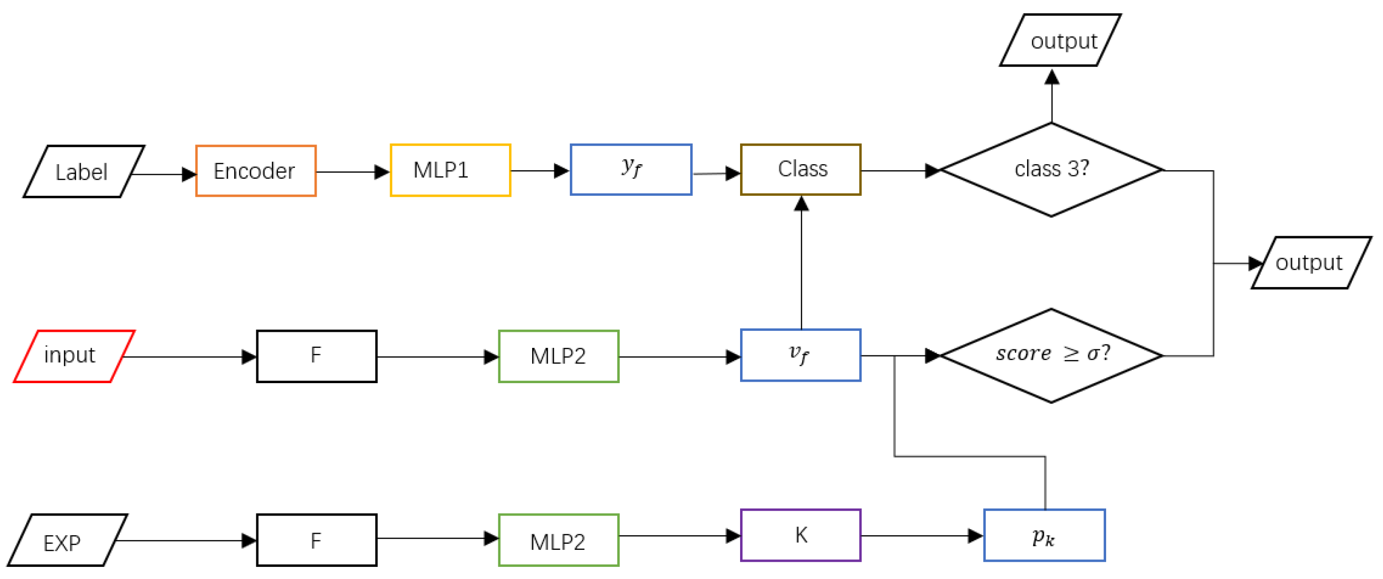
2.6. An Overview of the Detection Phase

As mentioned in the Introduction, bolts with pins are typically used for connecting tower body components to transmission line fittings, such as insulators, stay wire clamps, and grading rings. Consequently, BWPs and BLPs are often found at these fitting connection points. However, previous studies have not fully leveraged the correlation between fittings and bolts. Although the number of fitting categories is relatively small, the sample size for each type of fitting is also limited, making it impractical to annotate and classify each fitting individually. To overcome this issue, this study introduces an experience library, which is constructed by collecting 1000 images of BLPs and applying a clustering algorithm to obtain the category centers for different types of fittings. When the classifier identifies an image as Class 3 (BLP), it is further compared against the category centers for secondary verification to determine its true class. This process effectively serves as an unsupervised classification mechanism, utilizing clustering to derive the fitting category centers. By incorporating the inherent correlation between fittings and bolts, this method eliminates the challenges associated with individual annotation and classification while improving the accuracy of missing pin detection.
The network during the detection phase is illustrated in Figure 4. After the input module receives an image, it is processed by the previously trained F and the Translation Layer MLP2 to obtain the feature vector v f . The vector v f is then passed through the classifier to output a class target. This classifier calculates the similarity using the label vector y f , which was processed through the encoder and the Translation Layer MLP1. The similarity is computed via the dot product of the vectors, and the class with the highest similarity is output.
When the classifier predicts Class 1 (BP) or Class 2 (BWP), it directly outputs the result. If the prediction is Class 3 (BLP), the system will output BLP if the total score in the auxiliary branch exceeds the set threshold σ . If the classifier outputs BLP but the branch discrimination fails, the system will output BP.
The EXP branch of the empirical repository collects 1000 images with missing pins, which are similarly processed through the feature extraction module and the Translation Layer MLP2. The resulting feature vectors are clustered using K-means clustering [13,14] and aggregated into 100 classes p k to serve as sample centers for missing pins in the prior repository. The distance s i m k between the feature vector v f and the i -th sample center p k i is calculated using cosine similarity. The calculation formula is as follows:
s i m k = c o s θ = i = 1 n   v f i × p k i i = 1 n ( v f i ) 2 × i = 1 n ( p k i ) 2
The similarity score s i m k ranges from −1 to 1. If s i m k exceeds the predefined threshold γ , we consider the batch of samples to be similar to the class center p k in the empirical repository and assign 1 point. Similarly, by comparing it with other centers in the empirical repository EXP, a comprehensive score is obtained.
c o u n t k = 1     s i m k γ     0                                        
s c o r e = 1 100 c o u n t k
If the final score exceeds another threshold σ , i.e., s c o r e σ , the sample is considered to be a missing pin sample. The hyperparameters γ and σ involved in this process will affect the sensitivity of the branch discrimination.

2.7. Loss Function Calculation

2.7.1. Contrastive Learning Loss

Assuming the UNIS collects N samples per batch, after random augmentation, the number of samples doubles to 2 N . The vectors obtained after feature extraction and multilayer perceptron mapping are v f . These images undergo supervised contrastive learning pairwise, with their original label values y u s . The class distance is calculated through the dot product. The function l y u s i = y u s j takes the value 1 if the two samples have the same original label and 0 otherwise. The contrastive loss L c o n is defined as follows:
L c o n = 1 2 N 1 i = 1 2 N   j = 1 2 N l i j · l y u s i = y u s j · l o g e x p ( v f i · v f j / τ ) · e x p ( v f i · v f j / τ )

2.7.2. The Label Contrastive Loss of the Uniform Sampler

Assuming that the UNIS collects N samples per batch, with original label values y u s , where the labels are translated into vectors y f , and images are processed through feature extraction and translation to obtain feature vectors v f , the UNIS Contrastive Loss ( l u n i c o n ) is defined as follows:
L u n i c o n = 1 2 N i = 1 N   j = 1 N   l y u s i = y u s j · l o g e x p ( v f i · y f j / τ ) · e x p ( v f i · y f j / τ )

2.7.3. The Label Contrastive Loss of the Inverted Sampler

Assuming that the INVS collects N samples per batch, with original label values y i s , where the labels are translated into vectors y f , and images are processed through feature extraction and translation to obtain feature vectors v f , the INVS Contrastive Loss ( l i n v c o n ) is defined as follows:
L i n v c o n = 1 2 N i = 1 N   j = 1 N   l y i s i = y i s j · l o g e x p ( v f i · y f j / τ ) · e x p ( v f i · y f j / τ )

2.7.4. Overall Loss

The weights of the two samplers are dynamically weighted to form the label loss L l a b c o n :
L l a b c o n = t L i n v i c o n + ( 1 t ) L u n i c o n
The dynamic parameter t is defined as the square of the ratio of the current training epoch T to the total number of training epochs. That is,
t = ( T T m a x ) 2
The overall loss L of the network is the sum of the contrastive learning loss and the label loss.
L = L l a b c o n + α L c o n
The weight parameter α determines the relative weight between the contrastive learning loss and the label loss; τ is the temperature coefficient, and its value affects the model’s sensitivity to the differences between different types of data. The selection and impact of these two parameters will be further discussed in the subsequent experimental sections.

3. Results

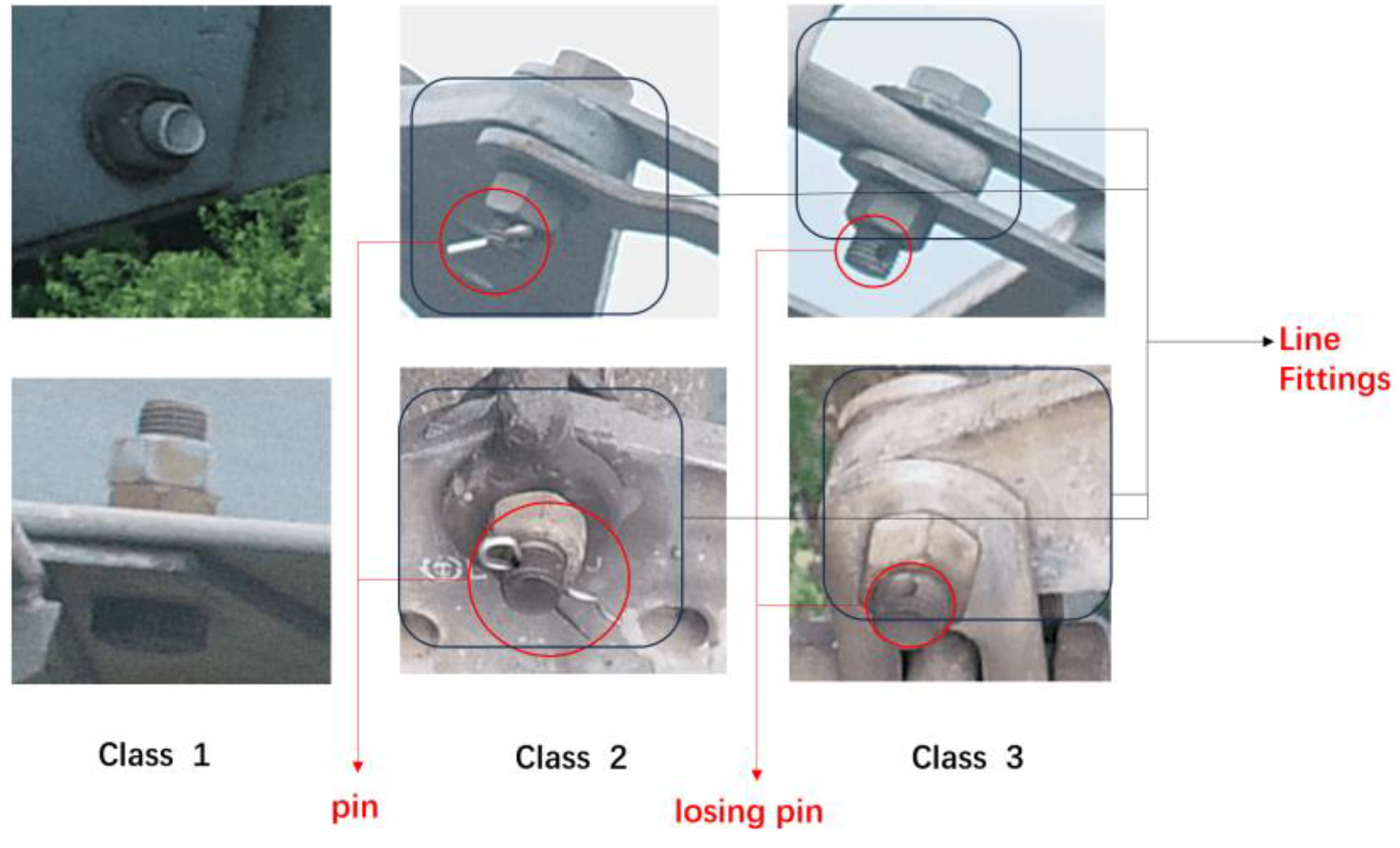
3.1. Introduction to the Dataset

The data used in this experiment are sourced from a certain company of the State Grid, using images captured by drones or fixed cameras. The bolt portion is cropped, and the preprocessed image size is 64 × 64. As shown in Figure 5, there are a total of 6413 original images of bolts, with 4227 images in Class 1 (BP), 1565 images in Class 2 (BWP), and 621 images in Class 3 (BLP), where the pin should be present but is missing. As can be seen, there is a severe imbalance in the sample sizes across different classes, and the smallest class, which has the fewest samples, happens to be the most difficult to recognize. As shown in Figure 5, pins are typically found at the connection points with the fittings. This experiment divides the dataset into training, validation, and test sets in a 7:2:1 ratio. Due to the small size of the dataset, to avoid random errors, the experimental data include five repeated tests with the random selection of the test set.

3.2. Experimental Setup

This experiment was conducted in a Windows environment, using a GeForce RTX 2080TI GPU (Nvidia, Santa Clara, CA, USA). The model was trained for 200 epochs with a batch size of 24. The software used was PyCharm, version 2023.2.5; and the experiment was run on the Pytorch framework, version 2.1. The Adam optimizer was used for training the model. The evaluation metric used in this experiment was accuracy (Acc), which reflects the overall classification accuracy of the model across all categories.
A c c u r a c y = T P + T F T P + T F + F P + F N
However, since the key Class 3 (missing pins) occupies a small proportion of the dataset, its impact on the OA (overall accuracy) is limited. Therefore, the precision and recall for Class 3 are reported separately to evaluate the improvement in prediction performance for this type of sample in this study.
P r e c e s i o n = T P T P + F P
R e c a l l = T P T P + F N

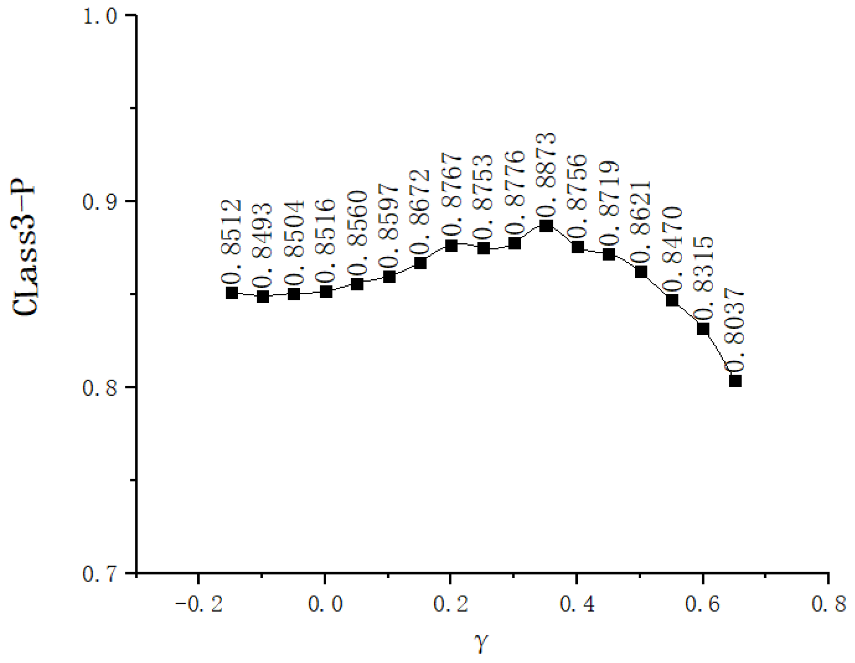
3.3. Hyperparameter Analysis

This experiment involves four hyperparameters: the cosine similarity threshold γ and the total score threshold σ from Section 2.6, as well as the weight parameter α of the inverted sampler and the temperature coefficient τ from Section 2.7.
The number of sample centers p k in the clustering algorithm, the total score threshold σ , and the similarity threshold γ are interrelated. Previous studies [9] have shown that when the number of category centers is too small, the representativeness of the sample library is significantly reduced. On the other hand, if the number of category centers is too large, it will considerably increase the computational burden of the auxiliary branch. When the proportion of the total score threshold σ relative to the total number of category centers is too small, the auxiliary branch loses its discriminative power; when the proportion is too large, it will incorrectly reject actual positive cases. However, when σ is set within an appropriate range, the search for γ will yield peak accuracy values that are close to each other. Based on empirical research, the total number of category centers is set to 100, and the total score threshold σ is set to 50. The optimal value for γ is searched within the range of (−1, 1) with a step size of 0.05. The detection metric used is the precision PPP for Class 3. The search results are shown in Figure 6, which lists the search outcomes around the peak value. The maximum precision for Class 3 occurs when γ = 0.35.
The weight parameter α affects the relative importance between the label contrastive loss L l a b c o n and the contrastive learning loss from random augmentation L c o n . The temperature coefficient τ determines the model’s sensitivity to the differences between samples. A smaller τ makes the model more sensitive to similarity differences, but this could also lead to large gradients or overfitting; a larger τ smooths the similarity distribution, leading to more stable training, but it may reduce the effectiveness of contrastive learning [12]. Based on empirical experience, the values of α and τ are searched within the range [0.01, 0.1, 1, 10, 100] in steps of 10. A finer search is then conducted around the peak value. The experimental results are shown in Table 1, with the evaluation metric being accuracy (Acc). The optimal experimental parameters are α = 1 and τ = 5.

3.4. The Results of the Control Group Experiments

This study uses dynamic weighting to balance the weights of the two samplers, combined with the Adam optimization algorithm. As shown in Equation (7), during the early stages of training, the weight of UNIS is larger, ensuring the model’s ability to fit the samples. In the later stages of training, the weight of INVS becomes larger, with smaller parameter adjustments, effectively fine-tuning the model based on UNIS, thus improving the fitting ability for BLP without losing the fitting capacity for the majority of the data. To investigate the impact of different weighting methods on the results, t in Equation (8) is replaced with different calculation methods, and the results are shown in Table 2.
When using a fixed weighting method, there is a certain improvement in the fitting ability for Class 3, but the fitting ability for the majority of the data is compromised, leading to a decrease in the overall model accuracy (Acc). This issue is particularly severe when t = 1 ( T T m a x ) 2 , where, despite achieving better results for Class 3, the overall model performance significantly declines. When the model applies dynamic weighting using a linear function, quadratic function, or cubic function, there are varying outcomes. This study selects the quadratic function weighting as it provides the best overall performance.
To verify the effectiveness of the proposed model, the control group for this experiment includes the following traditional classification networks: a ResNet18-based network with a softmax function, a ResNet18-based network combined with the Focal Loss function for imbalanced classification, and a ResNet18-based network using the LDAM loss function [15]. Additionally, a ResNet18-based network with a Swin Transformer [16] (using the tiny version due to the small dataset) is tested, employing the pretrained weights recommended on ImageNet. Our classification model is evaluated by comparing the impact of adding an auxiliary branch on computational resources and accuracy. The evaluation metric for computational resources, FPS, represents the number of images processed per second during both the training and inference stages. To validate the necessity of training a separate bolt classification model, we also selected the widely used Cascade-RCNN. (Since this network simultaneously performs both bolt localization and classification, only the classification accuracy of all detected bolts is recorded, and it is not meaningful to report the computation speed). The results in Table 3 show that although Focal Loss can somewhat alleviate the class imbalance issue, the overall performance improvement is limited due to the reduction in weight on the majority classes. While the Swin Transformer achieves a higher overall accuracy, this is based on pretrained weights, and its accuracy for the key class (missing pins) is only 0.7341. In contrast, our model shows a significant improvement in recognizing this class, achieving an accuracy of 0.8781.
From the results, it can be seen that although traditional two-stage methods achieve higher overall accuracy, they come at the cost of significant computational resources and have relatively poor prediction performance for the minority class, Class 3 (BLP). While the reweighted loss function can alleviate the imbalance issue to some extent, improving the accuracy of Class 3, the overall performance improvement is limited to 5–6% due to the reduced weight on the majority class. The Swin Transformer, while achieving higher overall accuracy, is based on pretrained weights and achieves only 0.7341 accuracy for the key category of missing pins. Our model, however, shows a significant improvement in recognizing this type of sample, reaching an accuracy of 0.8495.
In terms of computational resources, the reweighted approach has little effect on the computational requirements, as it simply adjusts the model’s focus on different types of data. For our model, during the training phase, both samplers work simultaneously and calculate contrastive loss with the label vectors, significantly increasing the computational burden. In traditional contrastive learning [12], a computation is required for each positive and negative sample pair, while in our approach (Equation (4)), only samples with the same label are considered as positive samples for contrastive loss calculation, which helps alleviate some of the computational pressure. Even so, our model’s per-image training cost is approximately eight times higher compared to the baseline framework. In the inference phase, before the Dual Branch is added, the inference cost is similar to that of the baseline framework. However, with the auxiliary branch, the inference cost per image increases by about five times for images that require it. Since such images make up a small proportion of the dataset, the overall average inference cost increases by about 40%. The auxiliary branch does not participate in training, so it has no impact on training costs.

3.5. Ablation Experiment

The ablation experiment results are shown in Table 4. Compared to the simple SimCLR contrastive learning network, the category label module, when used as the category center, improves the spatial distribution of feature vectors, leading to slight improvements across all metrics. The accuracy (Acc) increased by about 4%, and the recall for Class 3 improved by 6%. After adopting the dual-sampling method, the model’s predictive ability for the minority class, Class 3, significantly increased, with its precision rising by 37%. Since Class 1 and Class 3 are easily confused types, combining these two classes, along with the inclusion of category labels in the INVS, enhanced the differentiation between them, resulting in an additional 11% improvement in the recall for Class 3.
The changes in the confusion matrix after adding the auxiliary branch module are shown in Figure 7. The overall performance of the model changed little, with a slight 2% decrease in the recall for Class 3. This is because a small portion of the actual positives in Class 3 were rejected by the auxiliary branch. However, the probability of Class 1 (BP) being misclassified as Class 3 (BLP) was significantly reduced, with the false positive rate for BP being misclassified as BLP decreasing from 13% to 6%, reducing wasted human resources. Class 2 (BWP) did not participate in the branch discrimination and showed no significant change. The instances where BWP was misclassified as BLP mainly involved edge cases, where the pins were not missing but were severely damaged. These false positives do not completely constitute wasted effort for manual re-screening, as severely damaged pins should also be replaced.

4. Discussion

The bolt classification network proposed in this study completes the classification task in the pin detection process. To accomplish a full pin detection task, a lightweight Region Proposal Network (RPN) is also required. Inspired by Faster-RCNN, to reduce computational load, the Region Proposal Network and the classification network typically share the same backbone. Shallow features are used for the Region Proposal Network, while deep features are utilized for object classification and bounding box regression. The reason for using ResNet18 as the backbone in this study is also based on the fact that mainstream Faster-RCNN models typically use residual networks. Other networks, such as the Vgg16 series, would significantly increase the number of parameters when used as a backbone and make it difficult to train deep features. DenseNet, which uses dense connections, might offer similar computational efficiency to ResNet in single-head output tasks, but for multi-head output tasks, like Faster-RCNN, its dense connection characteristics would result in a substantial increase in computational load, whereas residual networks can avoid this issue. Future research may explore different backbone choices and improvements to balance multi-task output and computational efficiency.
In the auxiliary branch, the choice of hyperparameters for category centers was based on previous engineering experience from our team. The number of category centers does indeed have a significant impact on the computational efficiency of the auxiliary branch. In this study, the auxiliary branch significantly increased the inference speed per image; however, since only a small number of samples required the auxiliary branch, it had a minimal impact on the average inference speed. At the same time, the insufficient representativeness of the experience library led to the auxiliary branch incorrectly rejecting some actual positive samples, causing a slight decrease in the recall for Class 3. Improving the experience library can effectively reduce this occurrence. Therefore, future directions for the auxiliary branch are as follows: first, to explore the minimum number of category centers to reduce the computational load and second, to improve the clustering method to enhance the representativeness of the experience library, thus improving the accuracy of the auxiliary branch. Ideally, the auxiliary branch could establish a positive sample library to address false positives and reduce resource waste, as well as a negative sample library to handle false negatives and improve safety.
This study used random augmentation techniques in contrastive learning to address the small sample problem. However, these basic data augmentation methods provide limited improvement. In future research, we plan to consider using generative AI techniques such as GANs [17], which can not only effectively increase the sample size but also improve the feature distribution of the dataset, enhancing the model’s robustness to changes in environmental factors during actual inspection (such as lighting intensity, shooting angles, background noise, etc.). In the auxiliary branch, if GANs are used to effectively expand the positive sample library, it can improve the representativeness of the sample library and further reduce the probability of actual positives being incorrectly rejected by the auxiliary branch.

5. Conclusions

This study proposes a new approach for bolt classification in the pin detection field by training a separate bolt classification network and introduces a contrastive learning-based bolt classification network. For the first time, contrastive learning is applied to the field of transmission line bolt image classification, and the loss function is improved by calculating the contrastive loss for samples with the same label to reduce intra-class distance. This enhances the model’s ability to distinguish between similar features of samples with different labels, such as BP and BLP. Additionally, a category label module is introduced, which computes contrastive loss with images of the same category, increasing the inter-class distance and further improving the model’s ability to differentiate between images of different categories. Two samplers, UNIS and INVS, are used in combination with the Adam optimization algorithm, dynamically adjusting the weights of both samplers. This approach ensures that the model does not lose the features of majority-class data (BP) while enhancing its fitting ability for minority-class data (BLP) on the imbalanced dataset. The auxiliary branch utilizes unsupervised clustering to establish an experience library, employing a threshold-based decision mechanism to address the high false positive rate in the BLP category and reduce human resource waste in secondary inspection during transmission line inspection. Overall, the model improves the reliability of bolt image classification during UAV-based transmission line inspections. This model also has potential applications in other datasets with similar characteristics, such as class imbalance, small key feature pixel proportions, and limited sample sizes. The proposed auxiliary branch can be utilized in similar scenarios where certain background information and key features are related, reducing the probability of false positives or false negatives, but requires the establishment of a representative experience library for all true positives and true negatives.

Author Contributions

Conceptualization, Y.-P.J. and J.-L.Z.; methodology, L.-S.L.; software, J.-L.Z.; validation, H.-Y.F.; data curation, J.-Q.D.; writing—original draft preparation, Y.-P.J.; writing—review and editing, X.F. All authors have read and agreed to the published version of the manuscript.

Funding

This research was funded by the Power Science Research Institute of Hebei Electric Power Co., Ltd. (Project No. kj2023-005).

Data Availability Statement

Due to the First Affiliation’s data privacy policy, the dataset used is not publicly available.

Conflicts of Interest

The authors declare no conflicts of interest.

References

  1. Li, R.; Zhang, Y.; Zhai, D.; Xu, D. Pin Defect Detection of Transmission Line Based on Improved SSD. High Volt. Eng. 2021, 47, 3795–3802. [Google Scholar]
  2. Yi, H.; Liu, B.; Zhao, B.; Liu, E. Small Object Detection Algorithm Based on Improved YOLOv8 for Remote Sensing. IEEE J. Sel. Top. Appl. Earth Obs. Remote Sens. 2024, 17, 1734–1747. [Google Scholar] [CrossRef]
  3. Ren, K.; He, R.; Girshick, R. Faster R-CNN: Towards Real-Time Object Detection with Region Proposal Networks. IEEE Trans. Pattern Anal. Mach. Intell. 2016, 38, 1137–1149. [Google Scholar] [CrossRef] [PubMed]
  4. Cai, Z.W.; Vasconcelos, N. Cascade R-CNN: High Quality Object Detection and Instance Segmentation. IEEE Trans. Pattern Anal. Mach. Intell. 2021, 43, 1483–1498. [Google Scholar] [CrossRef] [PubMed]
  5. He, K.; Fan, H.; Wu, Y.; Xie, S.; Girshick, R. Momentum Contrast for Unsupervised Visual Representation Learning. In Proceedings of the IEEE/CVF Conference on Computer Vision and Pattern Recognition, Seattle, WA, USA, 13–19 June 2020; pp. 9726–9735. [Google Scholar]
  6. Snell, J.; Swersky, K.; Zemel, R. Prototypical Networks for Few-Shot Learning. In Proceedings of the Advances in Neural Information Processing Systems (NeurIPS), Long Beach, CA, USA, 4–9 December 2017. [Google Scholar]
  7. He, H.; Garcia, E.A. Learning from Imbalanced Data. IEEE Trans. Knowl. Data Eng. 2009, 21, 1263–1284. [Google Scholar]
  8. Lin, T.Y.; Goyal, P.; Girshick, R.; He, K.M.; Dollar, P. Focal Loss for Dense Object Detection. IEEE Trans. Pattern Anal. Mach. Intell. 2020, 42, 318–327. [Google Scholar] [CrossRef] [PubMed]
  9. Feng, T.; Liu, J.; Fang, X.; Wang, J.; Zhou, L. A Double-Branch Surface Detection System for Armatures in Vibration Motors with Miniature Volume Based on ResNet-101 and FPN. Sensors 2020, 20, 2360. [Google Scholar] [CrossRef]
  10. Chawla, N.V.; Bowyer, K.W.; Hall, L.O.; Kegelmeyer, W.P. SMOTE: Synthetic Minority Over-sampling Technique. J. Artif. Intell. Res. 2002, 16, 321–357. [Google Scholar] [CrossRef]
  11. He, K.; Zhang, X.; Ren, S.; Sun, J. Deep Residual Learning for Image Recognition. In Proceedings of the IEEE Conference on Computer Vision and Pattern Recognition (CVPR), Las Vegas, NV, USA, 27–30 June 2016; pp. 770–778. [Google Scholar]
  12. Chen, T.; Kornblith, S.; Norouzi, M.; Hinton, G. A Simple Framework for Contrastive Learning of Visual Representations. In Proceedings of the 37th International Conference on Machine Learning (ICML), Virtual, 13–18 July 2020; pp. 1597–1607. [Google Scholar]
  13. Ikotun, A.M.; Ezugwu, A.E.; Abualigah, L.; Abuhaija, B.; Heming, J. K-means Clustering Algorithms: A Comprehensive Review, Variants Analysis, and Advances in the Era of Big Data. Inf. Sci. 2023, 622, 178–210. [Google Scholar] [CrossRef]
  14. Liu, X.; Liu, X. SimpleMKKM: Simple Multiple Kernel K-Means. IEEE Trans. Pattern Anal. Mach. Intell. 2023, 45, 5174–5186. [Google Scholar] [CrossRef] [PubMed]
  15. Cao, K.D.; Wei, C.L.; Gaidon, A.; Arechiga, N.; Ma, T.Y. Learning Imbalanced Datasets with Label-Distribution-Aware Margin Loss. In Proceedings of the Advances in Neural Information Processing Systems 32 (NIPS), Vancouver, BC, Canada, 8–14 December 2019; Volume 32. [Google Scholar]
  16. Liu, Z.; Lin, Y.; Cao, Y.; Hu, H.; Wei, Y.; Zhang, Z.; Lin, S.; Guo, B. Swin Transformer: Hierarchical Vision Transformer using Shifted Windows. In Proceedings of the IEEE/CVF International Conference on Computer Vision (ICCV), Montreal, QC, Canada, 10–17 October 2021; pp. 10012–10022. [Google Scholar]
  17. Gozalo-Brizuela, R.; Garrido-Merchan, E.C. A Survey of Generative AI Applications. arXiv 2023, arXiv:2306.02781. [Google Scholar] [CrossRef]
Figure 1. Schematic diagram of training phase network. Explanation of abbreviations in image: UNIS (Uniform Sampling); INVIS (Inverse Sampling); x i s , x u s (image information of UNIS and INVS); y u s , y i s (label information of UNIS and INVS); x u s ’, x u s ” (two images obtained through random augmentation); Encoder (One-Hot Encoder); MLP1, MLP2 (multilayer perceptron); l u n i c o n (label contrastive loss of UNIS); l i n v c o n (label contrastive loss of INVS); l c o n (contrastive learning loss with random augmentation); l l a b c o n (overall label contrastive loss). The thick bidirectional arrows indicate that these module weights are shared.
Processes 13 00898 g001
Figure 2. Schematic diagram of contrastive learning.
Processes 13 00898 g002
Figure 3. Schematic diagram of category label module.
Processes 13 00898 g003
Figure 4. Schematic diagram of threshold alarm module. Explanation of newly introduced abbreviations: Label (label information); y f (processed label information vector); input (input image to be detected); v f (processed image information vector); EXP (images from experience library); K (K-means clustering);   p k (category centers obtained from processed reference library images).
Processes 13 00898 g004
Figure 5. Schematic of dataset.
Processes 13 00898 g005
Figure 6. The search results for the threshold γ .
Processes 13 00898 g006
Figure 7. Comparison of classification results after improvements.
Processes 13 00898 g007
Table 1. Experimental results of hyperparameters.
Hyperparameter α = 0.1 α = 0.5 α = 1.0 α = 5.0
τ = 0.1 0.90860.91280.91710.8936
τ = 1 0.90930.91660.91860.8967
τ = 5 0.91040.91720.91960.9005
τ = 10 0.91020.91850.91940.9015
Table 2. Results of different weighting methods.
t Overall AccuracyClass 3—PrecisionClass 3—Recall
0.50.72740.53650.6742
T T m a x 0.89140.86410.7891
( T T m a x ) 2 0.91960.88730.7707
1 ( T T m a x ) 2 0.62360.89150.8038
( T T m a x ) 3 0.85410.87470.7656
Table 3. The results of the control group experiments.
NameOverall AccuracyClass 3—PrecisionPredict FPSTrain FPS
Baseline0.85740.4751//
Resnet18-softmax0.75320.3283466.3195.4
Resnet18-Focal Loss0.81420.6919465.7193.6
ResNet18-LDAM Loss0.79830.7159466.1194.7
Swin Transformer0.87500.7341285.741.3
OURS without Dual Branch0.92270.8495406.223.7
OURS with Dual Branch0.91960.8873291.523.7
Table 4. The results of the ablation experiment.
NameOverall AccuracyClass 3—PrecisionClass 3—Recall
SimCLR-Resnet180.81740.41650.5595
SimCLR + Lable-contrast0.85720.42050.6131
SimCLR + Double Sampling0.90130.78260.6816
SimCLR + Lable-contrast + Dual-Sampling0.92270.84950.7905
SimCLR + Lable-contrast + Dual-Sampling + Dual-Branch0.91960.88730.7707
Disclaimer/Publisher’s Note: The statements, opinions and data contained in all publications are solely those of the individual author(s) and contributor(s) and not of MDPI and/or the editor(s). MDPI and/or the editor(s) disclaim responsibility for any injury to people or property resulting from any ideas, methods, instructions or products referred to in the content.

