Output Feedback Regulation via Sinusoidal Control with Application to Semi-Continuous Bio/Chemical Reactors

Abstract

This work proposes a nonlinear control strategy, an output feedback control based on a sinusoidal control approach for output regulation purposes with application to semi-continuous (fed-batch) bio/chemical processes. A key feature of the proposed control scheme is its auto-stop property, which ensures that the required set points are reached while automatically ceasing control input. This is particularly advantageous in fed-batch reactors, where exceeding the maximum operative volume is a common concern; additionally, the proposed controller can be bounded by only selecting the amplitude of the sine function. The closed-loop stability of the designed auto-stop control law is analyzed via the Lyapunov–Krazovzkii framework, which allows us to claim that the closed-loop dynamic operation of the corresponding processes is stable. The proposed controller is applied to two typical examples of semi-continuous bio/chemical reactors for regulation purposes, which aim to increase the reactors’ productivity. In addition, a comparison with a well-tuned internal model control proportional–integral (IMC PI) controller is performed. To show the performance of the control schemes, numerical experiments were carried out to show the controllers’ performance under different and realistic operation conditions. Here, for the bioreactor example, the performance index does not reach a steady state, but the gap between the IMC PI controller and the proposed one is around 100, 200, and 250 units for the different set points, which is in favor of the proposed controller. Regarding the chemical reactor, the performance index of the corresponding gap between the steady-state values of the performance index is also in favor of the proposed control law.

1. Introduction

Efficient and economical production via manufacturing processes has to consider several factors, for instance, the financial costs for media and supplements, the runtime of the processes, and particular operative issues in the bio/chemical industry, such as yield, product titer, and product quality [1]. Therefore, during process development, process engineers decide whether to apply a batch, semi-continuous, or continuous process [2,3].

In particular, fed-batch or semi-continuous fermentation is widely implemented as an operational option in the process industry, and it is a modified version of batch fermentation. There are many methods of adding a chemical reactive to the reactor; the right choice of feeding rate can improve performance considerably since it positively impacts the rate of product formation [4,5]. The foremost common feeding strategies are discontinuous feeding, achieved by regular or irregular pulses, and regular continuous feeding designed in step with a pre-calculated profile or by implementing a feedback controller supported by on-line measured variables [6,7].

For the operation of semi-continuous bio/chemical reactors, optimal control has been widely used as a control strategy, during which optimal trajectories of maximum productivity, minimum time operation, or optimal cost are sought [8,9,10]. Since optimal control actions are saturation-limited, optimal control consists usually of both singular and bang-bang arcs [11]. Generally, the control synthesis is based on accepted model knowledge and high-quality measurement of the most important state variables, which may be a serious drawback for realistic applications due to structural modeling errors and the lack of on-line measurements. The structure of the corresponding objective function to be minimized or maximized usually involves the nonlinear terms of the state variables and therefore a control effort to come up with the planning of the control law [12,13,14,15], which is another serious drawback. As mentioned above, there exist different controls for semi-continuous reactors, several of them related to optimization issues; however, for fed-batch reactors, the design of control strategies for output regulation purposes is not frequent. In particular, the regulation of mass concentration in a fed-batch operation is an important topic because designs where a specific concentration is reached in the reactors have a relevant impact on the reactors’ productivity. Moreover, adequate concentrations in this class of reactors allow for more efficient posterior operation units (for instance, separation of the compounds of interest in the reactive mixture) and a reduction in the energy requirements and consequently the costs of the operation of the subsequent separation processes.

The employment of trigonometric functions in the design of feedback control designs, as far as the authors know, is unexploited and unexplored in the work reported in the literature. Indeed, some of the few reports show how hyperbolic tangents have been employed instead of the discontinuous sign function under the framework of the sliding-mode theory [16,17,18]. Also, there are reports about the employment of hyperbolic functions during the training of algorithms in recurrent neural networks for feedback control, which has been frequently considered [12,19,20,21]. Also, in meta-heuristic optimization techniques, the sine–cosine algorithm (SCA) is a multi-agent-based optimization algorithm whose update roles are established based on the mathematical sine and cosine functions [22]; this methodology provides the optimal operation regions of the considered system, but this strategy is not an optimal controller.

In this contribution, a feedback control based on sinusoidal oscillatory function is explored for the output regulation of fed-batch bio/chemical reactors. In the following section, the main problem is described. In Section 3, the proposed feedback is detailed, which includes the closed-loop stability (via the Lyapunov–Krazovzkii framework) for the output regulation problem. Then, in Section 4, two examples are shown. The former regards a biochemical reactor whose kinetics represents substrate saturation (Monod kinetics) whereas the latter is an isothermal chemical reactor with Van de Vusse kinetics. Then, in Section 5, numerical experiments allow us to show and discuss the closed-loop performance. Finally, in Section 6, the text is closed with some concluding remarks.

2. Problem Statement

The control of semi-continuous processes presents unique challenges; for instance, the selected control input can only take values in a finite positive and closed interval F_in ∈ [0, F_max], F_max > 0, and the state vector x is real positive semi-definite, i.e., x ≥ 0. Furthermore, to derive a physically meaningful description, it will be considered that after the maximum level of liquid in the reactor’s tank V_max has been reached, the input flow F_in is automatically turned off to avoid overflow, which is a candidate for the control input. For any system variable x_i, let us denote its value at instant t as x_i(t, t₀, x₀, F) for any mass flow F, where x₀ = x₀(t₀) is the state at time t₀ ≤ t. It will also be assumed that the i-th kinetic reaction rates R_i’s are defined for x(t) ≥ 0, R_i (0) = 0 and are also positive (i.e., R_i > 0 for x(t) > 0), and bounded (i.e., R_i (x) ≤ $ℬ$ for every x(t) > 0 and for some positive constant $ℬ$), and the kinetic reaction rate $R_i\left(x\right)\in C^1,$ i.e., each reaction rate R_i is once continuously differentiable. Additionally, x_in will be considered not as a constant but as a variant quantity such that x_in(t) ≥ 0. It is operationally required that the concentration of a specific chemical compound in the reactor’s tank is below a specified level x_sp, while the reactor’s volume changes from the initial to final point, where 0 < V₀ < V_f ≤ V_max.

Therefore, the problem can be expressed as follows: To find a control law u for the input variable, i.e., u = F_in∈ [0, F_max], F_max > 0, which brings the system from a given state x₀ to a final condition x_f, in a set of desired final states x_f = {x_f | 0 ≤ x_min ≤ x(t) ≤ x_max}, by using an admissible input function along an admissible trajectory. Accordingly, regarding the physical conditions of the system, an input function is considered admissible if 0 ≤ F_in ≤ F_max, and when V = V_max, F_in = 0 for every finite time t > t₀ ≥ 0.

Some proposals for the control of semi-continuous reactors have considered PI regulators [23,24], adaptive controllers [25,26], and I/O linearizing control [27,28], among others [29]. In addition, a sinusoidal plus proportional control for regulation purposes with asymptotic and exponential convergence is proposed in [29]; however, this controller has several tuning parameters, which, considering the nonlinear nature of the controller and the process, make the corresponding tuning follow a trial-and-error process. As an example of the complex current problems, the optimal control of fed-batch bioreactor operation in real time could be considered. Here, some of the main problems that we can mention are the lack of on-line measurements of state variables that are crucial for evaluating the correct evolution of the process, the acquisition or even the development of specific sensors, and even the need to use state observers that must be coupled with the corresponding controllers as a technical challenge, in addition to the design of human–computer interfaces. For the above, research, development, and technological innovation are essential to solve the needs of today’s industry.

3. Control Design

Let us consider the following canonical nonlinear dynamic system with an affine control input:

$${\displaystyle \frac{dx}{dt}}=f\left(x\right)+g\left(x\right)u,$$

(1)

with a linear measurement equation, which is the system output:

$$y=Cx.$$

(2)

As usual, in Equations (1) and (2), x = [x₁(t),x₂(t),x₃(t) … x_n(t)]^T$\in {\mathbb{R}}^{\mathrm{n}}$ is the vector of state variables, such that [x₁(t),x₂(t),x₃(t),…, x_n(t)]$\mathrm{lies} \mathrm{at}$ $\mathcal{B}=\left\{x_i,i=1,2,\dots ,n|x_i\in \left[0x_{i,max}\right]\right\}$, where $\mathcal{B}$ is a compact set, i.e., $\mathcal{B}$ is bounded and closed under the vector field operations, y = [y₁(t),y₂(t),y₃(t) … y_p(t)]^T$\in {\mathbb{R}}^{\mathrm{p}}$ is the measurement vector with $p\le n,$ and u = [u₁(x₁) u₂(x₂) u₃(x₃) … u_q(x_q)]$\in {\mathbb{R}}^{\mathrm{q}}$ is the control input vector, with $q\le n$, f(x) = [f₁(x) f₂(x) f₃(x) … f_n(x)]^T; then, the function $f\left(x\right):{\mathbb{R}}^{\mathrm{n}}\to {\mathbb{R}}^{\mathrm{n}}$ defines a nonlinear and bounded smooth vector field, i.e., $‖f\left(x\right)‖\le \mathfrak{I}$, and $g\left(x\right)$: ${\mathbb{R}}^{\mathrm{n}}\to$ ${\mathbb{R}}^{\mathrm{n}\times \mathrm{q}}$ is a matrix that relates the control input and system output variables via state dynamics by using bounded relationships, i.e., is assumed that $‖g\left(x\right)‖\le \mathrm{\wp }$.

Proposition 1.

The following nonlinear control can regulate the output$y=Cx$of the system (1) at a constant $x_{sp}\in U\subset {\mathbb{R}}^n$: $u\in {\mathbb{R}}^q$whose components are given by

$$u_j=-k_{j-1}sin\left(k_j{e}_i\right),\mathrm{for} j = 1,2,3, \dots , q, \mathrm{and} i = 1,2,3,\dots , n,$$

(3)

where k_j-1 and k_j are control parameters, e_i = y_i − y_i,sp = x_i − x_i,sp is the regulation error, and y_i,sp = x_i,sp is a real constant.

Proof of Proposition 1.

Let us consider the closed-loop state equation of the system (1) under the controller (3), Then, by substituting (3) in (1), we find that, as y_i,sp = x_i,sp is constant, the components of the vector field for the regulation error e = y − y_sp = Cx − Cx_sp are given by

$${\displaystyle \frac{d{e}_i}{dt}}={\displaystyle \frac{d{x}_i}{dt}}=f_i\left(x\right)+g_i\left(x\right)k_{j-1}sin\left(k_j(x_i-x_{i,sp})\right), i = 1, 2, 3, \dots , n; j = 1,2,3, \dots , q.$$

(4)

Next, let us define the following function $h:{\mathbb{R}}^{\mathrm{n}}\to {\mathbb{R}}^{\mathrm{n}}$ such that its components are given by the right side of (4). Then, a linearized form of the nonlinear vector field $h\left(x\right)$ is obtained by applying a standard Taylor series linearization. Let us define

$$A\left(x\right)={\displaystyle \frac{\partial h}{\partial x}},$$

(5)

where $A\left(x\right)\in {\mathbb{R}}^{nxn}$ is the corresponding Jacobian matrix.

Then, at the neighborhood $U^0$ of the linearization point, $x^0$ becomes

$${\displaystyle \frac{de}{dt}}={\displaystyle \frac{dx}{dt}}\approx A\left(x\right)e\mathrm{for} x\in U^0.$$

(6)

Now, by considering Krasovskii’s method to analyze the local stability of the system (4), let us propose the following quadratic form of a candidate Lyapunov function:

$$V=h^{T}h.$$

(7)

Note that this scalar function is positive definite, and the time derivative of the scalar function V is given by

$$\dot{V}={\dot{h}}^{T}h+h^T\dot{h}.$$

(8)

From (5) and (6), due to the fact that $\dot{h}=A\left(x_{sp}\right)h$, we have

$$\dot{V}={\left(Ah\right)}^{T}h+h^{T}Ah,$$

(9)

and

$$\dot{V}=h^T\left(A^T+A\right)h.$$

(10)

Therefore, asymptotic stability can be ensured via the negativity of the matrix $Q=A^T+A$, that is, since

$$h\left(x\right)=f\left(x\right)+g\left(x\right)u\left(x\right),$$

(11)

the corresponding Jacobian matrix is given by

$$A\left(x\right)={\displaystyle \frac{\partial h}{\partial x}}=\left[\begin{array}{ccc}{\displaystyle \frac{\partial f_1}{\partial x_1}}& \cdots & {\displaystyle \frac{\partial f_1}{\partial x_n}}\\ ⋮& \ddots & ⋮\\ {\displaystyle \frac{\partial f_n}{\partial x_1}}& \cdots & {\displaystyle \frac{\partial f_n}{\partial x_n}}\end{array}\right]+\left[\begin{array}{ccc}{\displaystyle \frac{\partial {(g}_{11}{u}_1)}{\partial x_1}}& \cdots & {\displaystyle \frac{\partial {(g}_{11}{u}_1)}{\partial x_n}}\\ ⋮& \ddots & ⋮\\ {\displaystyle \frac{\partial {(g}_{nq}{u}_q)}{\partial x_1}}& \cdots & {\displaystyle \frac{\partial {(g}_{nq}{u}_q)}{\partial x_n}}\end{array}\right],$$

(12)

where

$${\displaystyle \frac{\partial {(g}_{ij}{u}_j)}{\partial x_i}}=u_j{\displaystyle \frac{\partial {(g}_{ij})}{\partial x_i}}+g_{ij}{\displaystyle \frac{\partial \left(u_j\right)}{\partial x_i}}.$$

(13)

Then, by accounting for Equation (13), we have that

$${\displaystyle \frac{\partial {(g}_{ij}{u}_j)}{\partial x_i}}=k_{i-1}sin\left(k_i{e}_i\right){\displaystyle \frac{\partial g_{ij}}{\partial x_i}}+g_{ij}{\displaystyle \frac{\partial \left(k_{i-1}sin\left(k_i{e}_i\right)\right)}{\partial x_i}},$$

(14)

$${\displaystyle \frac{\partial {(g}_{ij}{u}_j)}{\partial x_i}}=k_{i-1}sin\left(k_i{e}_i\right){\displaystyle \frac{\partial g_{ij}}{\partial x_i}}+g_{ij}{k}_{i-1}{k}_{i}cos\left(k_i{e}_i\right).$$

(15)

Finally, Equation (12) takes the form

$$A\left(x\right)=\left[\begin{array}{ccc}{\displaystyle \frac{\partial f_1}{\partial x_1}}& \cdots & {\displaystyle \frac{\partial f_1}{\partial x_n}}\\ ⋮& \ddots & ⋮\\ {\displaystyle \frac{\partial f_n}{\partial x_1}}& \cdots & {\displaystyle \frac{\partial f_n}{\partial x_n}}\end{array}\right]+$$

(16)

$$\left[\begin{array}{ccc}{k}_{0}Sin\left(k_1{e}_1\right){\displaystyle \frac{\partial g_{11}}{\partial x_1}}+g_{11}{k}_0{k}_{1}Cos\left(k_1{e}_1\right)& \cdots & k_{0}Sin\left(k_1{e}_1\right){\displaystyle \frac{\partial g_{11}}{\partial x_n}}+g_{11}{k}_0{k}_{1}Cos\left(k_1{e}_1\right)\\ ⋮& \ddots & ⋮\\ k_{n-1}Sin\left(k_n{e}_q\right){\displaystyle \frac{\partial g_{nq}}{\partial x_1}}+g_{nq}{k}_{n-1}{k}_{n}Cos\left(k_n{e}_q\right)& \cdots & k_{n-1}Sin\left(k_n{e}_q\right){\displaystyle \frac{\partial g_{nq}}{\partial x_n}}+g_{nq}{k}_{n-1}{k}_{n}Cos\left(k_n{e}_q\right)\end{array}\right]$$

Hence,

$$A\left(x_{sp}\right)={\left[\begin{array}{ccc}{\displaystyle \frac{\partial f_1}{\partial x_1}}& \cdots & {\displaystyle \frac{\partial f_1}{\partial x_n}}\\ ⋮& \ddots & ⋮\\ {\displaystyle \frac{\partial f_n}{\partial x_1}}& \cdots & {\displaystyle \frac{\partial f_n}{\partial x_n}}\end{array}\right]}_{x=x_{sp}}+{\left[\begin{array}{ccc}{g}_{11}{k}_0{k}_1& \cdots & g_{11}{k}_0{k}_1\\ ⋮& \ddots & ⋮\\ g_{nq}{k}_{n-1}{k}_n& \cdots & g_{nq}{k}_{n-1}{k}_n\end{array}\right]}_{x=x_{sp}}$$

(17)

$${A\left(x_{sp}\right)}^T={\left[\begin{array}{ccc}{\displaystyle \frac{\partial f_1}{\partial x_1}}& \cdots & {\displaystyle \frac{\partial f_n}{\partial x_1}}\\ ⋮& \ddots & ⋮\\ {\displaystyle \frac{\partial f_1}{\partial x_n}}& \cdots & {\displaystyle \frac{\partial f_n}{\partial x_n}}\end{array}\right]}_{x=x_{sp}}+{\left[\begin{array}{ccc}{g}_{11}{k}_0{k}_1& \cdots & g_{nq}{k}_{n-1}{k}_n\\ ⋮& \ddots & ⋮\\ g_{11}{k}_0{k}_1& \cdots & g_{nq}{k}_{n-1}{k}_n\end{array}\right]}_{x=x_{sp}}$$

(18)

$${Q=A\left(x_{sp}\right)}^T+A\left(x_{sp}\right)$$

(19)

$$Q=\left({\left[\begin{array}{ccc}{\displaystyle \frac{\partial f_1}{\partial x_1}}& \cdots & {\displaystyle \frac{\partial f_1}{\partial x_n}}\\ ⋮& \ddots & ⋮\\ {\displaystyle \frac{\partial f_n}{\partial x_1}}& \cdots & {\displaystyle \frac{\partial f_n}{\partial x_n}}\end{array}\right]}_{x=x_{sp}}+\left[\begin{array}{ccc}{g}_{11}{k}_0{k}_1& \cdots & g_{11}{k}_0{k}_1\\ ⋮& \ddots & ⋮\\ g_{nq}{k}_{n-1}{k}_n& \cdots & g_{nq}{k}_{n-1}{k}_n\end{array}\right]+\left({\left[\begin{array}{ccc}{\displaystyle \frac{\partial f_1}{\partial x_1}}& \cdots & {\displaystyle \frac{\partial f_n}{\partial x_1}}\\ ⋮& \ddots & ⋮\\ {\displaystyle \frac{\partial f_1}{\partial x_n}}& \cdots & {\displaystyle \frac{\partial f_n}{\partial x_n}}\end{array}\right]}_{x=x_{sp}}+\left[\begin{array}{ccc}{g}_{11}{k}_0{k}_1& \cdots & g_{nq}{k}_{n-1}{k}_n\\ ⋮& \ddots & ⋮\\ g_{11}{k}_0{k}_1& \cdots & g_{nq}{k}_{n-1}{k}_n\end{array}\right]\right)\right)$$

(20)

Finally, as observed, the parameters of the proposed control law $k_{i-1}{k}_i$ can be chosen (tuned) adequately to lead to the matrix Q being negatively defined. Consequently, the system (4) is asymptotically stable in the neighborhood around the selected set point x_sp. □

4. Application Examples

Now, the performance of the proposed control structure is evaluated via numerical experiments. To this end, two application cases are considered; both are bio/chemical reactors under the configuration of semi-continuous (fed-batch) operation.

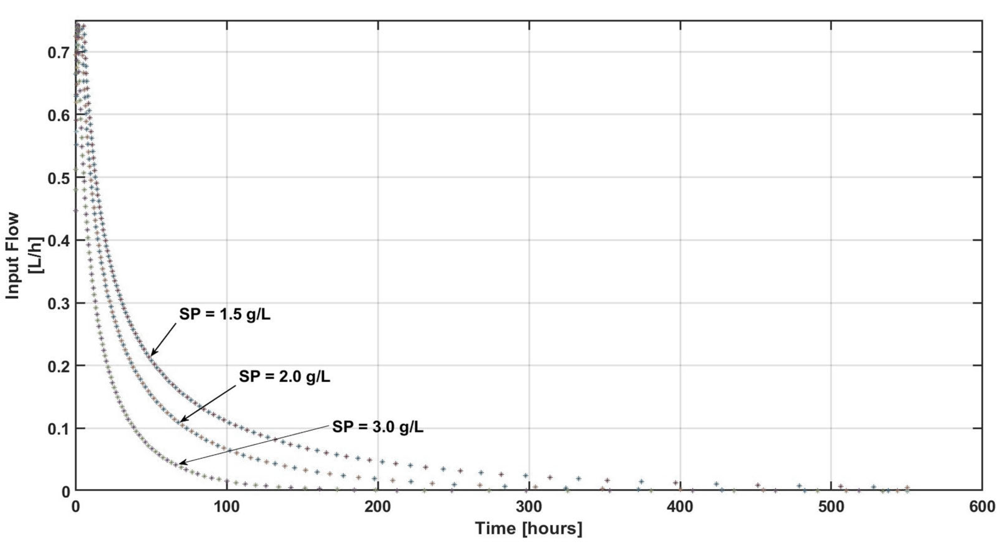
4.1. Biological Fed-Batch Reactor

The first application example is related to a generic bio/chemical reactor, where the kinetic model $\mu \left(x_1\right)$ is a Monod structure, with a variable coefficient yield $Y_s$, as follows:

$$\mu \left(x_1\right)={\mu }_{max}{\displaystyle \frac{x_1}{k_s+x_1}},$$

(21)

$$Y_s=\alpha +\beta x_1,$$

(22)

where $x_1$ is the substrate in the bio/chemical reactor, and for numerical experiments, we assume that µ_max = 0.3 h⁻¹, k_s = 1.75 gL⁻¹, α = 0.01 and dimensionless, β = 0.031 Lg⁻¹, and x_1,in = 20 gL⁻¹; see [30].

The kinetic models (21)–(22) are included within a mass balance equation, which describes the dynamical behavior of the substrate and biomass concentrations and the bioreactor’s volume:

$${\displaystyle \frac{d{x}_1}{dt}}=-{\displaystyle \frac{\mu \left(x_1\right)x_2}{Y_s}}+\left(x_{1,in}-x_1\right){\displaystyle \frac{u}{x_3}},$$

(23)

$${\displaystyle \frac{d{x}_2}{dt}}=\mu \left(x_1\right)x_2-x_2{\displaystyle \frac{u}{x_3}},$$

(24)

$${\displaystyle \frac{d{x}_3}{dt}}=u,$$

(25)

where $x_1$, $x_2$, and $x_3$ are the substrate, biomass, and volume in the bio/chemical reactor. The control command input stands for the scalar that represents the flow

u = 2.25 sin (0.1e),

(26)

where e = x₂ − x_2,sp is the regulation error and x_2,sp is the required set point.

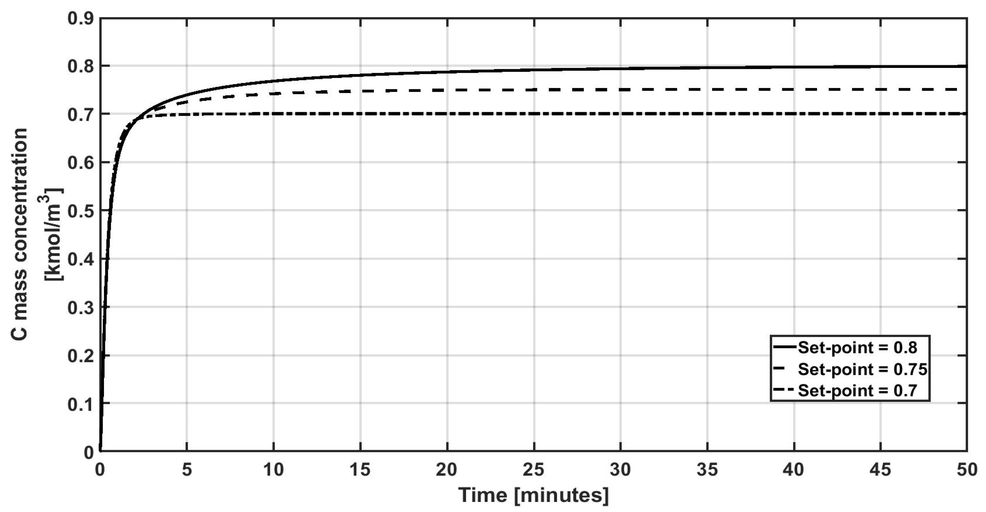
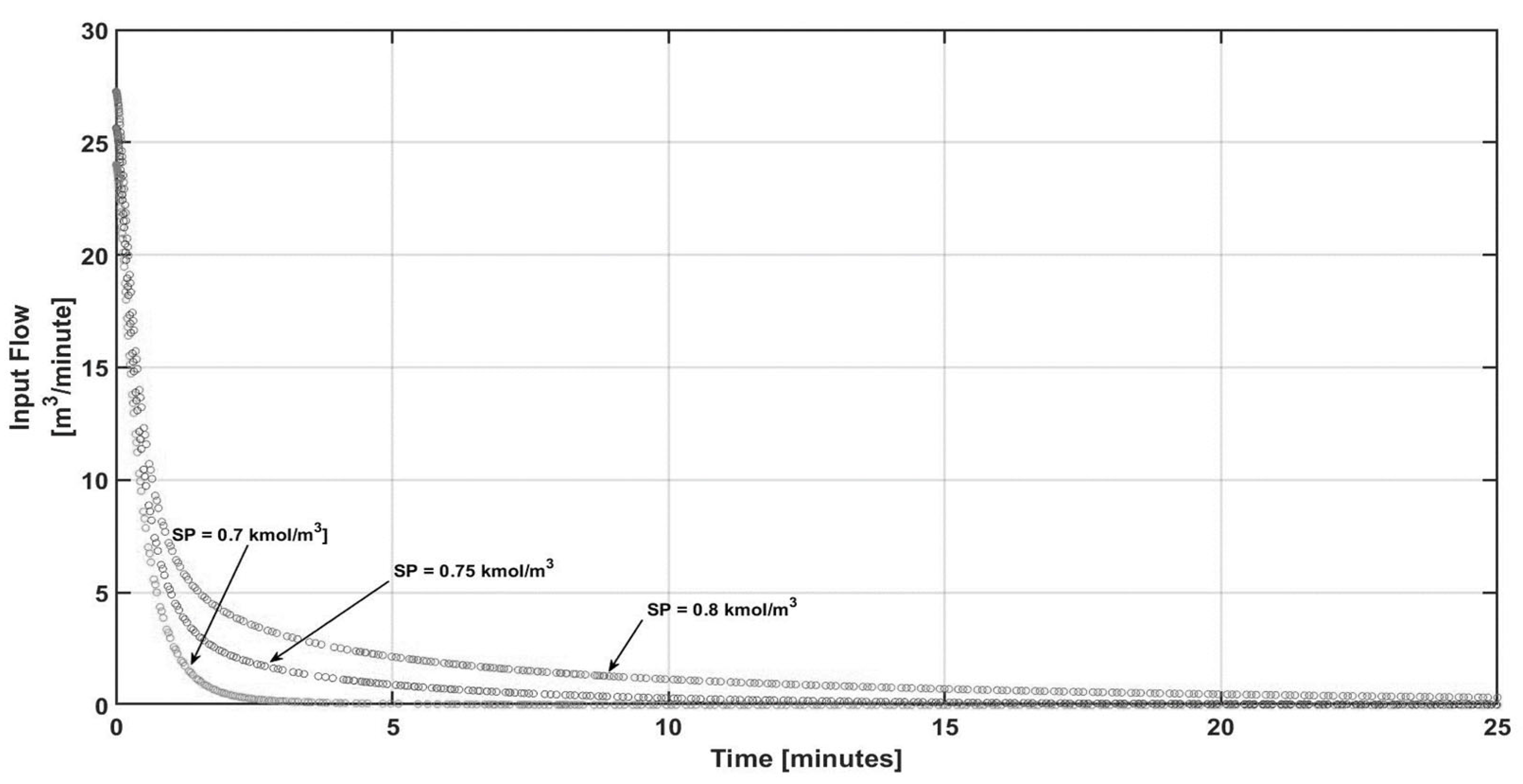
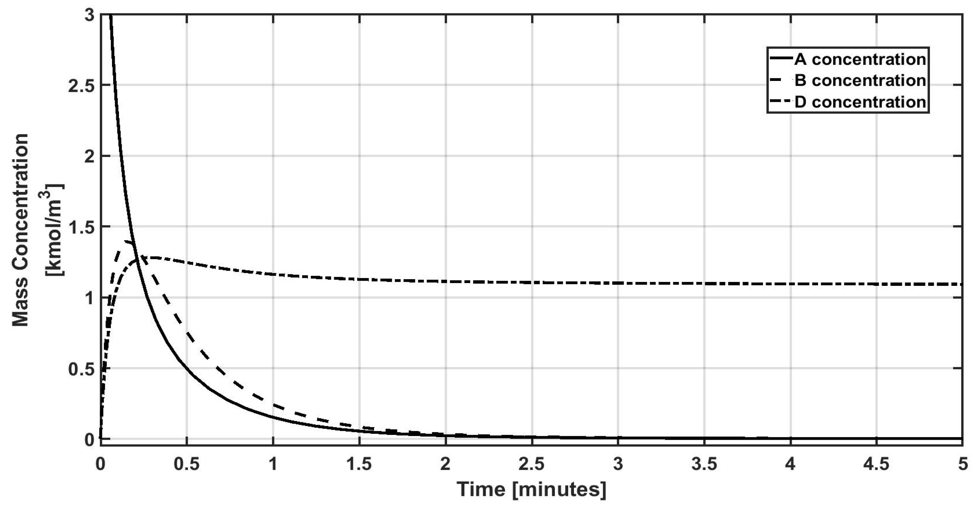
4.2. Chemical Fed-Batch Reactor

The second case is related to an isothermal representation of the Van de Vusse chemical reaction; these chemical reactions include a parallel and series reaction kinetic pathway, which are represented by a power-law kinetic model.

The mass balance equations for the chemical reactor are given by

$${\displaystyle \frac{d{C}_A}{dt}}={\displaystyle \frac{u_c}{V}}\left(C_{Ain}-C_A\right)-k_1{C}_A-k_3{C}_A^2,$$

(27)

$${\displaystyle \frac{d{C}_B}{dt}}=-{\displaystyle \frac{u_c}{V}}{C}_B+k_1{C}_A-k_2{C}_B,$$

(28)

$${\displaystyle \frac{d{C}_C}{dt}}=-{\displaystyle \frac{u_c}{V}}{C}_C+k_2{C}_B,$$

(29)

$${\displaystyle \frac{d{C}_D}{dt}}=-{\displaystyle \frac{u_c}{V}}{C}_D+k_3{C}_A^2,$$

(30)

$${\displaystyle \frac{dV}{dt}}=u_c,$$

(31)

where $k_i\left(T\right)=k_{i0}exp\left(-{\displaystyle \frac{E_i}{RT}}\right),fori=1,2,3$, $C_A$, $C_B$, $C_C$ and $C_D$ are mass concentrations, V is the volume, and the control command input $u_c$ denotes the inlet flow, with

u_c = −70 Sin (0.2 e)

(32)

with e = C_C − C_C,sp as the regulation error.

Here, k₁₀ = 2.145 × 10¹⁰ min⁻¹, k₂₀ = 2.145 × 10¹⁰ min⁻¹ and k₁₀ = 2.145 × 10¹⁰ min⁻¹. E₁/RT = 9758.3 K, E₂/RT = 9758.3 K and E3/RT = 8560 K; see [15].

5. Numerical Results and Discussion

Numerical experiments were carried out to show the performance of the proposed methodology, using a PC with an Intel 7I Core processor and employing the MATLAB R2024b library ode23s to solve the corresponding set of ordinary differential equations.

On the output regulation of the bioreactor: Regarding the regulation of the bioreactor model, a single-input–single-output control configuration is assumed; the control goal is to lead the biomass concentration to different set points, which are x_2,sp = 1.5 g/L, x_2,sp = 2.0 g/L, and x_2,sp = 3.0 g/L. Biomass concentration is assumed to be measured on-line; this is a realistic assumption because there are several devices available commercially to obtain these kinds of measurements, such as devices based on turbidimetric and dielectric techniques [31].

Figure 1 shows the closed-loop performance of the biomass concentration under the proposed controller. It can be noted that the proposed methodology can reach the distinct set points smoothly. Coupled with the first figure, in Figure 2, the control effort required for the proposed control law for each one of the corresponding set points is observed. Note that the controller is such that the volumetric flow converges during a longer-term operation time, when the required set point is related to a small concentration. This fact can be explained in the sense that the controller dilutes the biomass concentration via the inlet volumetric flow. This issue can be analyzed in Figure 3; indeed, because the control input is the inlet volumetric flow, the reactor’s volume increases due to the inlet volumetric flow. In other words, since the set point is related to small concentrations, in order to reach a biomass concentration of x_2,sp = 1.5 g/L, the reactor’s volume in steady state is around 52 L; in contrast, for x_2,sp = 2.0 g/L, the reactor’s volume in steady state is around 38 L, and, finally, when x_2,sp = 3.0 g/L, the reactor’s volume in steady state is close to 28 L.

For a whole picture of the bioreactor’s behavior, a closed-loop phase portrait is shown in Figure 4. Here, the performance of the state variables under different initial conditions can be observed; notice that in all the cases, the controller leads to the control output (biomass concentration) being at the required set point (sp = 3 g/L), and all the trajectories arrive at the required set point across smooth curves.

Now, for comparison purposes, an IMC proportional–integral (IMC PI) controller is considered. An IMC PI controller is a type of controller that uses the internal model control strategy, specifically designed to be implemented with a proportional–integral (PI) controller. IMC is a popular control strategy in process control due to its simplicity, robustness, and ability to handle model uncertainties effectively.

Generally, the IMC PI controller is relatively simple to implement, as it uses a model-based control strategy with PI terms that are easy to tune, offering good performance for many systems without the complexity of a full PID controller [32].

The performance of the IMC PI controller can be optimized to provide fast response times, minimal overshoot, and no steady-state error by adjusting the proportional and integral gains. The IMC controller is robust to plant–model mismatches and disturbances. Even if the model is not perfectly accurate, the controller can still maintain good performance. In addition, the controller provides accurate tracking of the set point, especially in the presence of disturbances or slow dynamics [33,34,35].

As mentioned above, IMC PI controllers have been successfully employed in chemical reactors, distillation columns, temperature control in industrial systems, and flow rate regulation [36,37].

For our application case, the IMC PI tuning rules given in [38] are considered and the corresponding controller’s parameters are k_p = 0.2 h⁻¹ and τ_I = 3.85; by observing Figure 5, the performance of the PI controller shows an oscillatory behavior, with high overshoots, around 2 g/L, and a large settling time of 250 h; in comparison, the proposed methodology presents non-oscillatory behavior, without overshoots and a settling time of around 100 h.

Performance comparisons of the proposed methodology and the PI controller, for the different set points considered as application examples, are shown in Figure 6, Figure 7 and Figure 8 for the corresponding set point values of sp₁ = 3 g/L, sp₂ = 2 g/L, and sp₃ = 1.5 g/L, respectively. The mentioned comparison is performed via the performance index $IAE={\int }_0^{t}abs\left[e\left(\tau \right)\right]d\tau$. It can be noticed that the proposed methodology has better performance, in all cases, than the PI controller.

The Van de Vusse isothermal chemical reactor: Next, the second application case, which is related to a chemical reactor with an isotherm Van de Vusse kinetic, is considered. This case is assumed under isotherm conditions, with T = 100° C as the operation temperature. To illustrate a realistic operation case, the chemical compound C, which is an intermediate compound of the chemical network, is selected as a controlled variable; in this way, it is assumed that compound C is available via on-line measurements or soft sensors. As in the bioreactor, three different set points are selected to show the regulative capacities of the proposed methodology: C_sp = 0.7 mol/L, C_sp = 0.75 mol/L, and C_sp = 0.8 mol/L.

Figure 9 shows the closed-loop performance of the C concentration under the proposed controller for distinct arbitrary set points. Note the smooth response of the corresponding trajectories to reach the required set point concentrations; here, it can be seen that the proposed control law is able to regulate the reactor’s operations.

Figure 10 is included to show the whole performance of the dynamic behavior of the uncontrolled concentrations, where the smooth and stable behavior of the state variables of this system is observed. That is to say, the control implementation shows that the output feedback regulation via the proposed controller involves internal stability because the state vector reaches a stable steady state. It is relevant to mention the difficult operation needed to reach the corresponding set points for the C compound. Considering its intermediate compound nature, the corresponding selectivity for the reaction network is hard to manipulate.

Now, from the abovementioned, the proposed controller effort acts to increase the reactor’s volume via the input flow for the different required set points, as is depicted in Figure 11 and Figure 12.

Furthermore, a comparison with an IMC PI controller is also performed; its corresponding control gains k_p = −11 min⁻¹, and τ_I = −7.35 in accordance with the IMC tuning rules proposed in [38]. Figure 13 shows the performance of the PI controller versus the proposed methodology; the PI controller shows oscillatory behavior, with an overshoot of 0.05 kmol/m³ and a large settling time of 42 min. The proposed control law does not show an overshoot, and the settling time is around 2 min for the selected set point of 0.7 kmol/m³.

A comparison of the closed-loop performance of the proposed and PI controllers is realized by employing, as a performance index, the absolute values of the regulation error integral, $IAE={\int }_0^{t}abs\left[e\left(\tau \right)\right]d\tau .$ In Figure 14, Figure 15 and Figure 16, a performance comparison is performed with different set points considered as application cases: sp₁ = 0.7 kmol/m³, sp₂ = 0.75 kmol/m³, and sp₃ = 0.8 kmol/m³, respectively. As observed, the proposed methodology has better performance.

Possible resonance as an additional concern: Next, a concern regards the oscillatory nature of the proposed controller. Further simulations are included considering sustained disturbances in the A concentration at the input condition, as A_in = A_in0 + 1.25 Sin(10t), and a noisy measurement for the biomass concentration of ± 5% from the biomass concentration current value. The steady state is demonstrated and illustrated via numerical experiments. Since the reactor’s behavior is autonomous in the sense that it only depends on the output and set point (there is no time dependence), the possible resonance phenomena can be attributable to fluctuation in the control error e = y − y_sp = Cx − Cx_sp. Since the set point Cx_sp is time-invariant, the source of a possible fluctuation in control error can be found at the output measurements y = Cx. Of course, resonance is a concern because oscillatory behavior in the reactor state vector is undesirable.

To explore how possible resonance can be avoided when the proposed controller is interconnected via feedback, a set of numerical experiments have been realized to account for the effect of noisy measurements on the closed-loop performance. Figure 17 and Figure 18 correspond to the closed-loop regulation in noisy environments during biomass concentration measurements. Note that the control command is insensitive (see Figure 17) to the control input and shows fluctuations as consequence of the noise. Seeking completeness, noisy concentration measurements for the intermediate compound were simulated; see Figure 19 and Figure 20.

The results in Figure 17, Figure 18, Figure 19 and Figure 20 suggest acceptable closed-loop performance on the regulated variable. However, a detailed investigation into these concerns is recommendable, which unfortunately is beyond the aim of this contribution.

6. Concluding Remarks

The main contribution of this work is to present an alternative design of a nonlinear controller with a sinusoidal structure; an important feature of the proposed control scheme is its auto-stop property, which ensures that the required set points are reached while automatically ceasing control input. This is advantageous in fed-batch reactors, where exceeding the maximum operative volume is a common concern; in addition, the proposed controller can be bounded by only selecting the amplitude of the sine function. The regulation of the closed-loop system was performed in a smooth way, considering the smoothness of the proposed control structure and the compactness and boundedness of the systems under study. For the abovementioned characteristics, the proposed methodology seems to be adequate for semi-continuous or feedback chemical reactors and their operational characteristics. The sinusoidal controller was applied to two typical examples of chemical reactors, a chemostat-type bioreactor and a chemical reactor with a complex reaction network, with success. The proposed methodology has better performance in comparison with a well-tuned IMC PI controller, which is one of the best methodologies of the PID control family for the regulation and tracking of smooth systems. As a future work, a theoretical closed-loop analysis of the amplitude and phase of the sine function acting as a control input and numerical experiments must be performed to show their impact on the closed-loop dynamic performance of the chemical reactors.

References

1. Liu, J.; Ren, J.; Yang, Y.; Liu, X.; Sun, L. Effective semicontinuous distillation design for separating normal alkanes via multi-objective optimization and control. Chem. Eng. Res. Des. 2021, 168, 340–356. [Google Scholar] [CrossRef]
2. Madabhushi, P.B.; Adams, T.A., II. Side stream control in semicontinuous distillation. Comput. Chem. Eng. 2018, 119, 450–464. [Google Scholar] [CrossRef]
3. Shen, Y.; Forrester, S.; Koval, J.; Urgun-Demirtas, M. Yearlong semi-continuous operation of thermophilic two-stage anaerobic digesters amended with biochar for enhanced biomethane production. J. Clean. Prod. 2017, 167, 863–874. [Google Scholar] [CrossRef]
4. Ripoll, V.; Agabo-García, C.; Solera, R.; Perez, M. Modeling of the anaerobic semi-continuous co-digestion of sewage sludge and wine distillery wastewater. Environ. Sci. Water Res. Technol. 2020, 6, 1880–1889. [Google Scholar] [CrossRef]
5. Miramontes-Martínez, L.R.; Gómez-González, R.; Botello-Álvarez, J.E.; Escamilla-Alvarado, C.; Albalate-Ramírez, A.; Rivas-García, P. Semi-continuous anaerobic co-digestion of vegetable waste and cow manure: A study of process stabilization. Rev. Mex. De Ing. Química 2020, 19, 2020. [Google Scholar] [CrossRef]
6. Bresaola, M.D.; Morocho-Jácome, A.L.; Matsudo, M.C.; de Carvalho, J.C. Semi-continuous process as a promising technique in Ankistrodesmus braunii cultivation in a photobioreactor. J. Appl. Phycol. 2019, 31, 2197–2205. [Google Scholar] [CrossRef]
7. Murillo, C.; Irakoze, G.; de Oliveira Vigier, K.; Delmas, M.; Jérôme, F.; Pérès, Y.; Urrutigoity, M.; Cognet, P. Modeling of Ethylene Glycol Production from Glucose in a Semi-Continuous Reactor. Chem. Eng. Technol. 2020, 43, 950–963. [Google Scholar] [CrossRef]
8. Breton-Deval, L.; Méndez-Acosta, H.O.; González-Álvarez, V.; Snell-Castro, R.; Gutiérrez -Sánchez, D.; Arreola-Vargas, J. Agave tequilana bagasse for methane production in batch and sequencing batch reactors: Acid catalyst effect, batch optimization and stability of the semi-continuous process. J. Environ. Manag. 2018, 224, 156–163. [Google Scholar] [CrossRef]
9. Johnson, A. The control of fed-batch fermentation processes. A survey. Automatica 1987, 23, 691–705. [Google Scholar] [CrossRef]
10. De Battista, H.; Jamilis, M.; Garelli, F.; Picó, J. Global stabilization of continuous bioreactors: Tools for analysis and design of feeding laws. Automatica 2018, 89, 340–348. [Google Scholar] [CrossRef]
11. Jäschke, J.; Cao, Y.; Kariwala, V. Self-optimizing control—A survey. Annu. Rev. Control 2017, 43, 199–223. [Google Scholar] [CrossRef]
12. Ammar, Y.; Cognet, P.; Cabassud, M. ANN for hybrid modeling of batch and fed-batch chemical reactors. Chem. Eng. Sci. 2021, 237, 116522. [Google Scholar] [CrossRef]
13. Rätze, K.; Jokiel, M.; Kaiser, N.M.; Sundmacher, K. Cyclic operation of a semi-batch reactor for the hydroformylation of long-chain olefins and integration in a continuous production process. Chem. Eng. J. 2019, 377, 120453. [Google Scholar] [CrossRef]
14. Dovžan, D.; Škrjanc, I. Predictive functional control based on an adaptive fuzzy model of a hybrid semi-batch reactor. Control Eng. Pract. 2010, 18, 979–989. [Google Scholar] [CrossRef]
15. Aguilar-López, R.; Mata-Machuca, J.L.; Godinez-Cantillo, V. A TITO Control Strategy to Increase Productivity in Uncertain Exothermic Continuous Chemical Reactors. Processes 2021, 9, 873. [Google Scholar] [CrossRef]
16. Figueroa-Estrada, J.C.; Neria-González, M.I.; Rodríguez-Vázquez, R.; Tec-Caamal, E.N.; Aguilar-López, R. Controlling a continuous stirred tank reactor for zinc leaching. Miner. Eng. 2020, 157, 106549. [Google Scholar] [CrossRef]
17. Lara-Cisneros, G.; Aguilar-López, R.; Dochain, D.; Femat, R. On-line estimation of VFA concentration in anaerobic digestion via methane outflow rate measurements. Comput. Chem. Eng. 2016, 94, 250–256. [Google Scholar] [CrossRef]
18. Aguilar-López, R.; Mata-Machuca, J.L.; Martínez-Guerra, R.; Pérez-Pinacho, C.A. Synchronization of Multiple Mechanical Oscillators Under Noisy Measurements Signals and Mismatch Parameters. Int. J. Nonlinear Sci. Numer. Simul. 2017, 19, 699–707. [Google Scholar] [CrossRef]
19. Poznyak, A.; Chairez, I.; Poznyak, T. A survey on artificial neural networks application for identification and control in environmental engineering: Biological and chemical systems with the uncertain model. Annu. Rev. Control 2019, 48, 250–272. [Google Scholar] [CrossRef]
20. Esche, E.; Weigert, J.; Brand, G.; Göbel, R.; Repke, J. Architectures for neural networks as surrogates for dynamic systems in chemical engineering. Chem. Eng. Res. Des. 2022, 177, 184–199. [Google Scholar] [CrossRef]
21. Kirilova, E.G. Artificial Neural Networks: Applications in Chemical Engineering. In Modeling and Simulation in Chemical Engineering: Project Reports on Process Simulation; Boyadjiev, C., Ed.; Springer International Publishing: Cham, Switzerland, 2022; pp. 127–146. [Google Scholar]
22. Mirjalili, S. SCA: A Sine-Cosine Algorithm for solving optimization problems. Knowl.-Based Syst. 2016, 96, 120–133. [Google Scholar] [CrossRef]
23. Webster, T.A.; Hadley, B.C.; Dickson, M.; Busa, J.K.; Jaques, C.; Mason, C. Feedback control of two supplemental feeds during fed-batch culture on a platform process using inline Raman models for glucose and phenylalanine concentration. Bioprocess Biosyst. Eng. 2021, 44, 127–140. [Google Scholar] [CrossRef] [PubMed]
24. Kager, J.; Tuveri, A.; Ulonska, S.; Kroll, P.; Herwig, C. Experimental verification and comparison of model predictive, PID, and model inversion control in a Penicillium chrysogenum fed-batch process. Process Biochem. 2020, 90, 1–11. [Google Scholar] [CrossRef]
25. Galvanauskas, V.; Simutis, R.; Vaitkus, V. Adaptive control of biomass specific growth rate in fed-batch biotechnological processes. A comparative study. Processes 2019, 7, 810. [Google Scholar] [CrossRef]
26. Roy, S.; Chopda, V.; Gomes, J.; Rathore, A.S. Comparison and implementation of different control strategies for improving production of rHSA using Pichia pastoris. J. Biotechnol. 2019, 290, 33–43. [Google Scholar]
27. Panjapornpon, C.; Saksomboon, P.; Juyteiy, K.; Chinprasit, J. Input/output linearization for a real-time pH control: Application on basic wastewater neutralization by carbon dioxide in a fed-batch bubble column reactor. Eng. J. 2019, 23, 229–241. [Google Scholar] [CrossRef]
28. Chopda, V.; Rathore, A.S.; Gomes, J. On-line implementation of decoupled input-output linearizing controller in Baker’s yeast fermentation. IFAC Proc. Vol. 2013, 46, 259–264. [Google Scholar] [CrossRef]
29. Aguilar-López, R.; González-Viveros, I.; López-Pérez, P.A. Sinusoidal control strategy applied to continuous stirred-tank reactors: Asymptotic and exponential convergence. Can. J. Chem. Eng. 2025, 103, 744. [Google Scholar] [CrossRef]
30. Gomez-Acata, R.V.; Lara-Cisneros, G.; Femat, R.; Aguilar-López, R. On the dynamic behavior of a class of bioreactor with non-conventional yield coefficient form. Rev. Mex. De Ing. Química 2015, 14, 149–165. [Google Scholar]
31. Díaz Pacheco, A.; Delgado-Macuil, R.J.; Díaz-Pacheco, Á.; Larralde-Corona, C.P.; Dinorín-Téllez-Girón, J.; López-López, V.E. Use of equivalent circuit analysis and Cole–Cole model in evaluation of bioreactor operating conditions for biomass monitoring by impedance spectroscopy. Bioprocess Biosyst. Eng. 2021, 44, 1923–1934. [Google Scholar] [CrossRef]
32. Ravikumar, C.; Sivakumar, D. Design and Simulation of IMC Based PI Controller for a MIMO Process. Int. J. Sci. Res. Sci. Technol. 2018, 4, 57–63. [Google Scholar]
33. Besta, C.S.; Chidambaram, M. Control of Unstable Multivariable Systems by IMC Method. In Proceedings of the 2017 Trends in Industrial Measurement and Automation (TIMA), Chennai, India, 6–8 January 2017; pp. 1–6. [Google Scholar]
34. Pathiran, A.R. Improving the Regulatory Response of PID Controller Using Internal Model Control Principles. Int. J. Control Sci. Eng. 2019, 9, 9–14. [Google Scholar]
35. Ahmadi, A.H.; Nikravesh, S.K.; Moradi Amani, A. A Unified IMC Based PI/PID Controller Tuning Approach for Time Delay Processes. AUT J. Electr. Eng. 2020, 52, 31–52. [Google Scholar]
36. Diwakar, B.; Anandh, M.G.; Brinda, R.; Devi, S.J.; Aravind, P. IMC Based Design of PI Controller for Real Time Pressure Process. Int. J. Innov. Res. Electr. Electron. Instrum. Control Eng. 2015, 3, 12–15. [Google Scholar]
37. Seki, H. Self-Tuning IMC-PI Controllers for Chemical Process Applications. In Proceedings of the 2016 IEEE Conference on Control Applications (CCA), Buenos Aires, Argentina, 19–22 September 2016; pp. 1179–1184. [Google Scholar]
38. Ogunnaike, B.A.; Ray, W.H. Process Dynamics, Modeling, and Control; Oxford University Press: New York, NY, USA, 1994. [Google Scholar]
Figure 1. Closed-loop performance of the control output under different set points.
Processes 13 00891 g001
Figure 2. Control effort under different set points.
Processes 13 00891 g002
Figure 3. Dynamic response of the reactor’s volume under different set points.
Processes 13 00891 g003
Figure 4. Closed-loop phase portrait under different initial conditions.
Processes 13 00891 g004
Figure 5. Performance comparison of an IMC PI control and the proposed control.
Processes 13 00891 g005
Figure 6. Dynamic evolution of the performance index for the IMC PI controller and the proposed controller for a set point = 3 g/L.
Processes 13 00891 g006
Figure 7. Dynamic evolution of the performance index for the IMC PI controller and the proposed controller for a set point = 2 g/L.
Processes 13 00891 g007
Figure 8. Dynamic evolution of the performance index for the IMC PI controller and the proposed controller for a set point = 1.5 g/L.
Processes 13 00891 g008
Figure 9. Closed-loop performance of the control output under different set points.
Processes 13 00891 g009
Figure 10. Control effort under different set points.
Processes 13 00891 g010
Figure 11. Closed-loop performance of the uncontrolled variables.
Processes 13 00891 g011
Figure 12. Dynamic response of the reactor’s volume under different set points.
Processes 13 00891 g012
Figure 13. Performance comparison of an IMC PI control and the proposed control.
Processes 13 00891 g013
Figure 14. Dynamic evolution of the performance index for the IMC PI controller and the proposed controller for a set point = 0.7 kmol/m3.
Processes 13 00891 g014
Figure 15. Dynamic evolution of the performance index for the IMC PI controller and the proposed controller for a set point = 0.75 kmol/m3.
Processes 13 00891 g015
Figure 16. Dynamic evolution of the performance index for the IMC PI controller and the proposed controller for a set point = 0.8 kmol/m3.
Processes 13 00891 g016
Figure 17. Dynamic response of the control output under sustained disturbances and noisy measurements.
Processes 13 00891 g017
Figure 18. Dynamic response of the control input under sustained disturbances and noisy measurements.
Processes 13 00891 g018
Figure 19. Dynamic response of the control output under sustained disturbances and noisy measurements.
Processes 13 00891 g019
Figure 20. Dynamic response of the control input under sustained disturbances and noisy measurements.
Processes 13 00891 g020
Disclaimer/Publisher’s Note: The statements, opinions and data contained in all publications are solely those of the individual author(s) and contributor(s) and not of MDPI and/or the editor(s). MDPI and/or the editor(s) disclaim responsibility for any injury to people or property resulting from any ideas, methods, instructions or products referred to in the content.