Power System Loss Reduction Strategy Considering Security Constraints Based on Improved Particle Swarm Algorithm and Coordinated Dispatch of Source–Grid–Load–Storage

Abstract

Coordinating various controllable distributed resources to reduce network losses is crucial to the secure and economical operation of modern power systems. This paper proposes a bi-level optimization model for power system loss reduction based on “source-grid-load-storage” coordinated optimization. The upper level aims to minimize the total annual planning cost of the system, determining the location and capacity of distributed photovoltaic systems, energy storage devices, and electric vehicle charging stations. The lower level aims to minimize the load curve smoothness and node voltage deviation of the distribution network, optimizing intraday operation strategies. For this complex optimization problem, this paper designs a particle swarm optimization (PSO) algorithm with adaptive weights and improved evolutionary strategies. The simulation results of case studies demonstrate that the proposed method has significant loss reduction effects in distribution networks of various scales and complexities. The algorithm performance comparison results show that the improved particle swarm algorithm outperforms traditional algorithms in terms of solution quality and computational efficiency, providing an effective solution for the coordinated optimization of “source-grid-load-storage”.

1. Introduction

To achieve “dual carbon” targets, large-scale renewable energy has been integrated into modern power systems, which has a significant influence on the secure and economical operation of power systems [1]. Positioned at the end of the power system and facing the consumers directly, the distribution network facilitates the integration of a massive amount of distributed renewable energy and the flexible management of user-side loads, serving as a crucial component of the modern power systems [2]. With the substantial incorporation of high proportions of renewable energy and new types of loads, cumulative energy losses within the power system become significant, with network losses in medium- and low-voltage distribution networks accounting for approximately 80% of the total system losses [3]. Therefore, in the context of large-scale construction of distribution networks, how to coordinate the various controllable distributed resources within these networks to enhance the consumption capacity of renewable energy in the distribution grid, reduce network losses, improve voltage quality, and thereby achieve secure and economical operation of the power system is of significant importance [4].

Addressing this important issue, researchers both domestically and internationally have conducted extensive studies, covering mixed-integer second-order cone programming, distributed coordinated optimization, statistical comprehensive evaluation techniques, and the application of machine learning algorithms in distribution network loss optimization [5]. Reference [6] employs mixed-integer second-order cone programming for multi-objective optimization of distribution network losses, voltage, and demand response utilization. This research not only enhances system operational efficiency and reliability but also fully leverages the value of demand-side flexibility resources, providing novel technical approaches and decision support for economical and efficient distribution network operation. However, the mixed-integer second-order cone optimization methodology may encounter challenges of high computational complexity and extended solution times when applied to practical large-scale distribution networks. Reference [7] addresses the non-convex characteristics presented by the active and reactive power coordinated optimization model for distribution networks, proposing a distributed active and reactive power coordinated optimization method that considers the model’s non-convex nature, effectively reducing network losses. However, given that the issue of network losses in distribution networks involves multiple aspects, such as sources, grids, loads, and storage, and factors like changes in theoretical network loss calculation boundary conditions caused by the introduction of a high proportion of power electronic devices, there remains a need to develop loss reduction strategies suitable for the new type of distribution networks [8].

With the maturation of “source-grid-load-storage” coordinated optimization and statistical comprehensive evaluation techniques, experts and scholars domestically and internationally have considered utilizing these technologies to explore the potential for loss reduction in distribution networks. Reference [9] establishes a fuzzy evaluation model for economic operation of distribution networks based on interval number theory, achieving the multi-dimensional quantitative assessment of grid economic performance, effectively identifying system weaknesses, and providing a scientific basis for optimization decisions and precise improvements in distribution networks. Reference [10] innovatively combines static and dynamic indicators to construct an energy efficiency assessment system for medium-voltage distribution networks. It proposes an integrated no-loss rate as the core loss assessment indicator to correct underestimations of loss rates. Although this method innovatively introduces dynamically changing indicators, it faces real-time data collection and processing challenges. Reference [11] builds an energy efficiency assessment system for grid loss reduction under “load-network-source” coordinated control, comprehensively evaluating the effectiveness of grid loss reduction. Although these studies have made progress in the construction of evaluation systems, there is still room for improvement in the comprehensive coordination of source–grid–load–storage.

With the rapid development of machine learning technologies, emerging theories and techniques have been applied to loss reduction in distribution networks. Reference [12] utilizes a quantum genetic algorithm to optimize the training parameters of support vector machines, enhancing the accuracy of distribution network loss calculations. This method excels in addressing small-sample, nonlinear, and high-dimensional pattern recognition problems, but it is not suitable for large-scale data. Reference [13] proposes a two-stage optimization method for the dynamic reconfiguration of distribution networks with distributed generation (DG), integrating biogeography-based algorithms to effectively address the complexity and practicality issues of distribution network reconfiguration, achieving a significant reduction in active power losses and providing more efficient network topology optimization strategies for modern distribution networks with distributed energy resources. However, the biogeography-based algorithm is slow, resulting in high computational costs. Reference [14] improves the particle swarm optimization algorithm by using dynamic inertia weights to study and analyze the impact of DG integration on network losses. This optimization algorithm can reasonably select inertia weights and will likely obtain optimal solutions. However, it still faces limitations, such as sensitivity in parameter selection, leading to less-than-ideal problem-solving outcomes.

Therefore, under the premise of “source-grid-load-storage” coordinated planning, this paper constructs a bi-level optimization model for loss reduction in distribution networks. The key innovations of this paper can be summarized as follows:

(1)

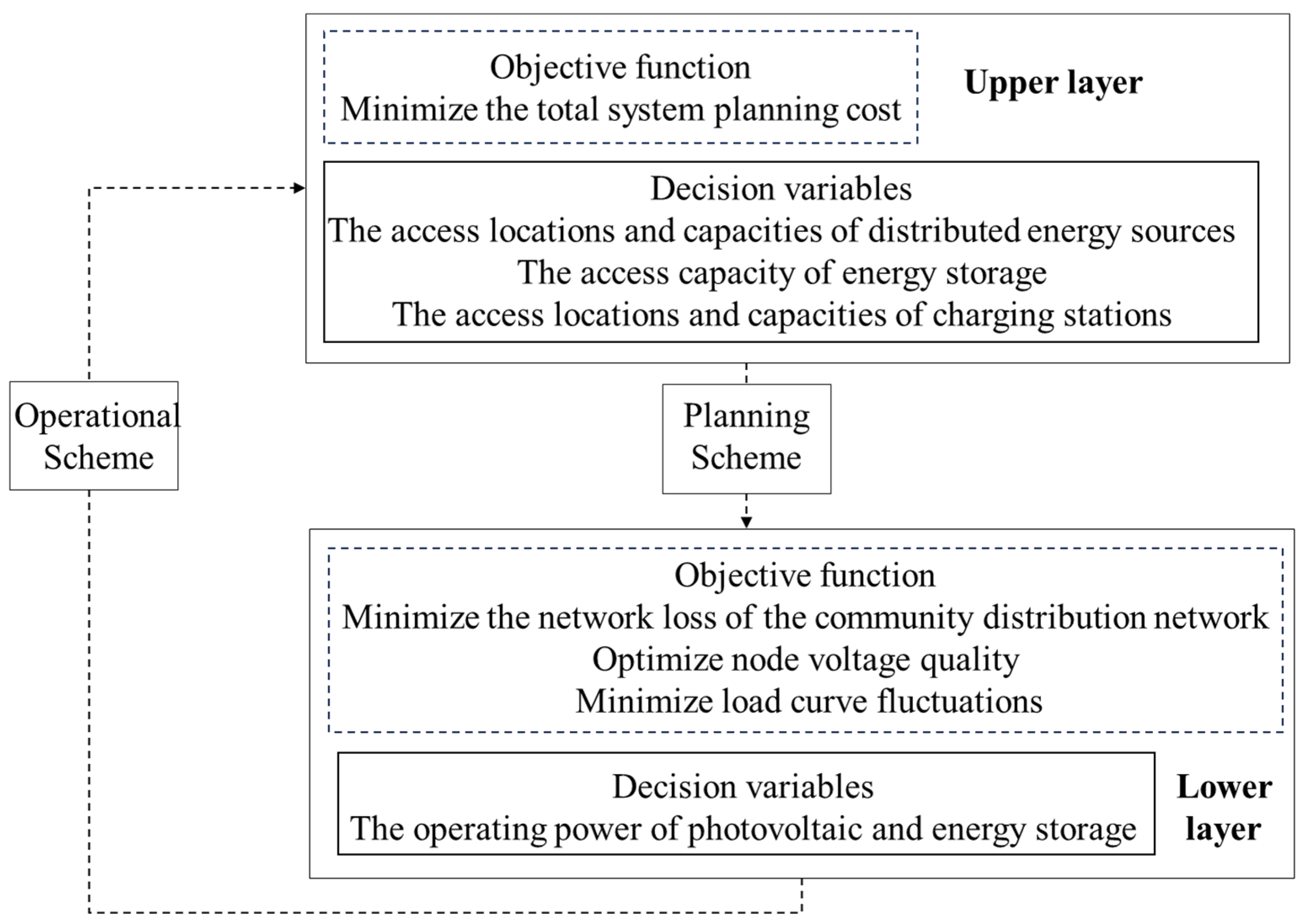
A bi-level optimization model is proposed for addressing distribution network loss reduction. The upper-level objective minimizes the total annual planning cost, while the lower-level objectives focus on minimizing both the load curve variance and the node voltage deviation. By considering economic efficiency and operational characteristics at both global and local levels, this model provides a theoretical foundation for the collaborative optimization of loss reduction strategies.

(2)

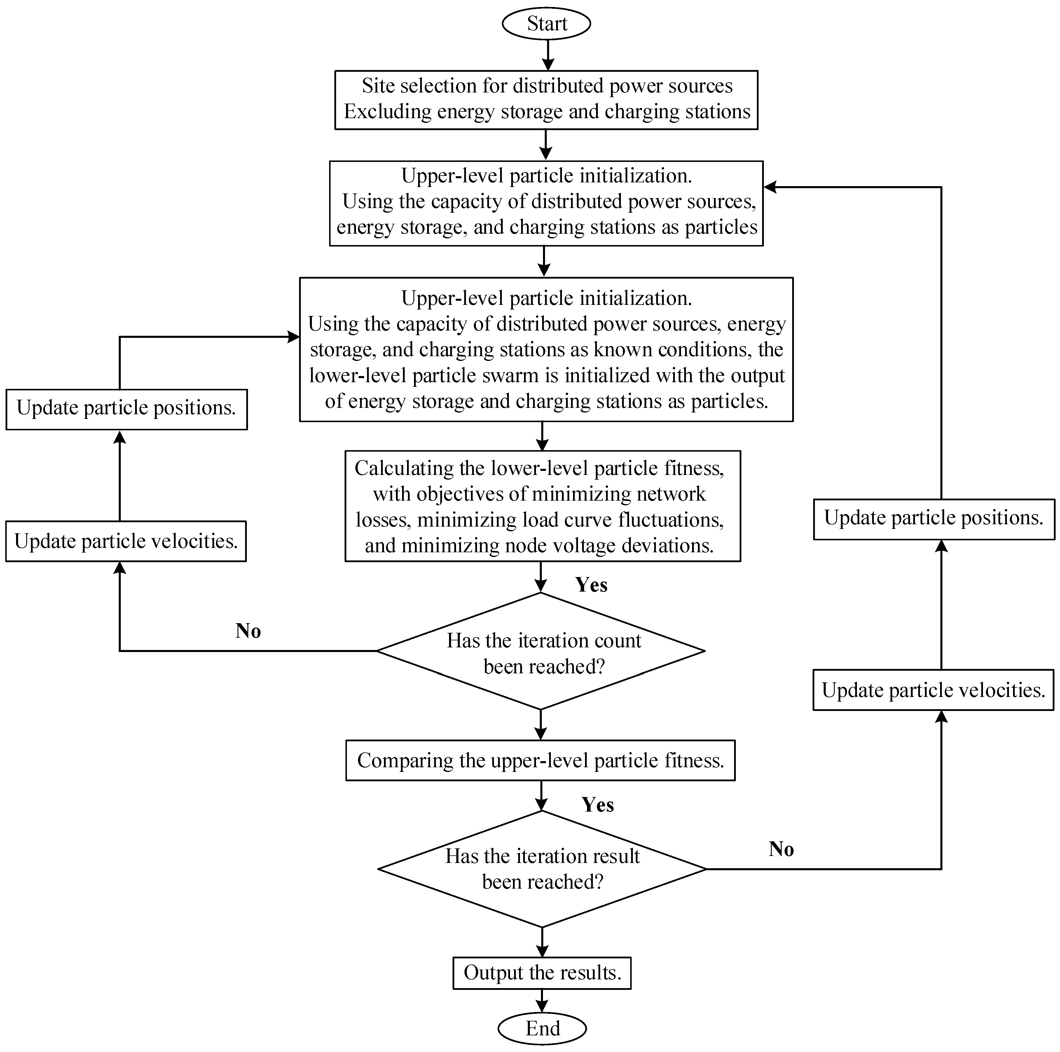
In response to the constructed bi-level optimization model, this paper proposes and applies an improved particle swarm optimization algorithm. The results demonstrate the algorithm’s superior performance in terms of search speed and convergence accuracy, thereby confirming the effectiveness and feasibility of the proposed method for distribution network loss reduction optimization.

The remainder of this paper is organized as follows: Section 2 presents the interaction mechanism of the “source-grid-load-storage” in distribution networks along with models for distributed photovoltaic power sources, network restructuring, energy storage, and load models. Section 3 analyzes the factors affecting power losses in distribution networks. Section 4 introduces an improved particle swarm optimization algorithm. Section 5 establishes a dual-layer optimization model for power loss reduction in distribution networks coordinated by “source-grid-load-storage”, and Section 6 provides case study analyses. Section 7 concludes the paper.

2. Model of the Distribution Network

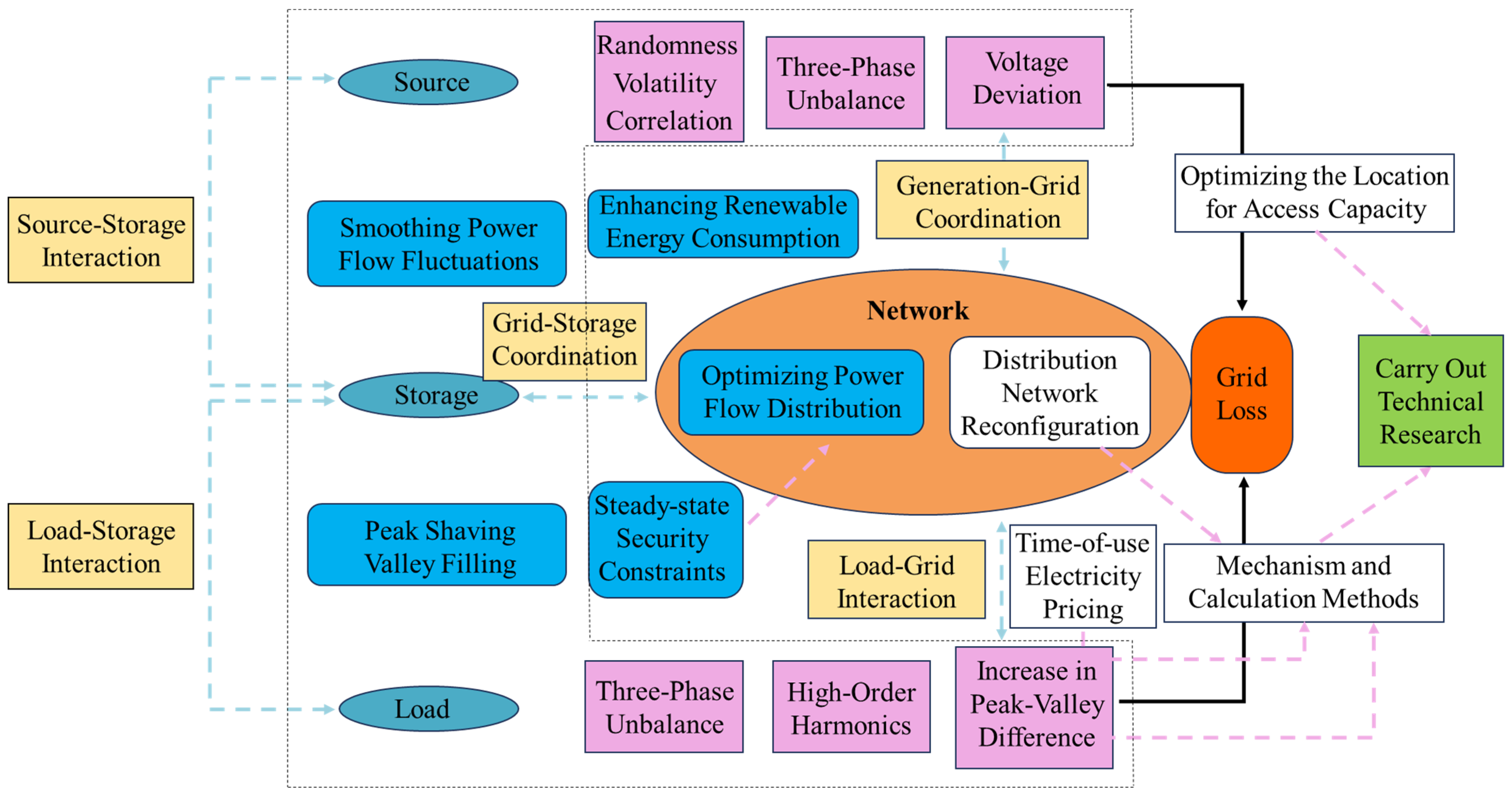
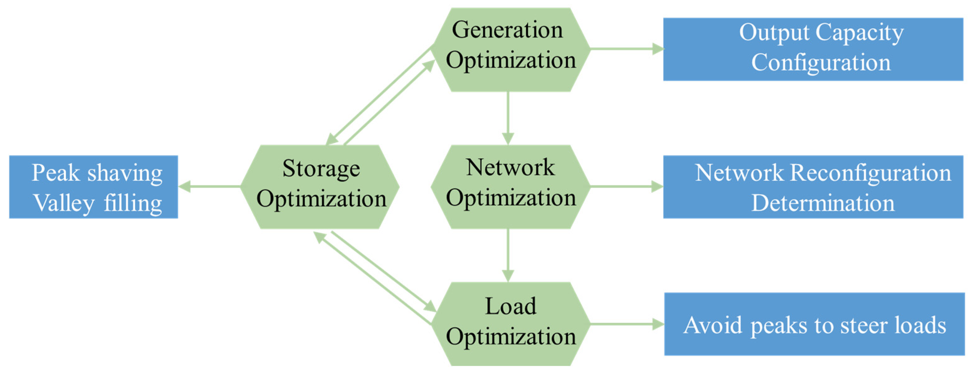
2.1. The Interaction Mechanism of “Source-Grid-Load-Storage” in the Distribution Network

Figure 1 shows the coordinated interaction of source–grid–load–storage in the distribution network, which includes four parts: controllable distributed generation, energy storage devices, controllable resources for distribution network reconfiguration, and demand response loads.

Source: Optimize the output of distributed generation, taking into account the complementary characteristics of output timing and spatial distribution to reduce the impact of power fluctuations on the power quality of the distribution network. Enhance the consumption of renewable energy, optimize the capacity and siting of DG to balance as much as possible locally, reduce the flow of grid currents, decrease network losses, and improve the economic efficiency of grid operations.

Grid: Optimizing power flow distribution through network reconfiguration under power system steady-state security constraints, balance line loads, conserve energy and reduce losses, and improve the quality of reactive power and voltage.

Load: Analyze the potential for load control and the complementary characteristics between the source and load curves. Guide user consumption habits through electricity pricing to reduce peak load, alleviate network congestion, and decrease network losses.

Storage: With rapid charging and discharging capabilities to mitigate power fluctuations, swiftly track the output of distributed energy sources, improve power quality, and enhance the consumption of renewable energy.

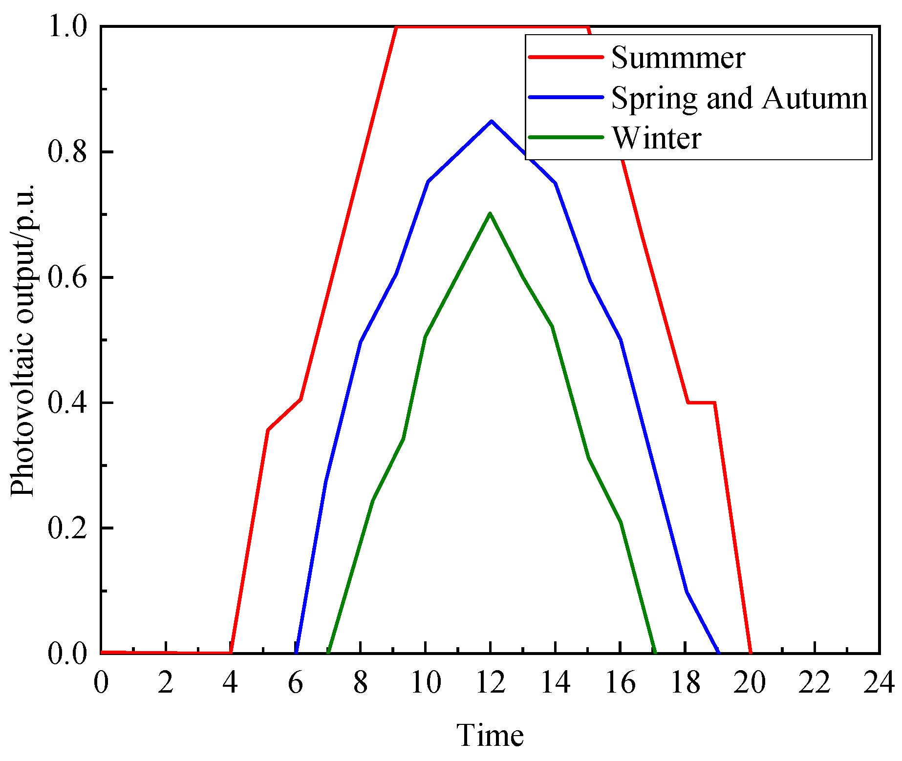
2.2. Model of Distributed Photovoltaic Power Source

In this paper, the distributed photovoltaic (PV) power source is represented by a PV cell circuit model [15]. The output power at a given time t is primarily influenced by the temperature of the PV cell T_cell(t), the ambient temperature T_en(t), and the solar irradiance S(t). The relationship among these three factors can be expressed by (1).

$$T_{cell}(t)=T_{en}(t)+S(t)\cdot {\displaystyle \frac{T_{no}-20}{0.8}}$$

(1)

where T_no is the rated battery operating temperature.

At time t, the active power output P_PV(t) of the PV cell, along with the output voltage U_PV(t) and current I_PV(t), can be expressed by (2).

$$\left\{\begin{array}{l}{P}_{PV}(t)={\alpha }_F\cdot U_{PV}(t)\cdot I_{PV}(t)\\ {\alpha }_F={\displaystyle \frac{U_{MPP}{I}_{MPP}}{U_{oc}{I}_{sc}}}\\ U_{PV}(t)=U_{oc}-K_V\cdot T_{cell}(t)\\ I_{PV}(t)=S(t)\cdot [I_{sc}+K_I\cdot (T_{cell}(t)-25)]\end{array}\right.$$

(2)

where α_F is filling factor; U_MPP and I_MPP are the voltage and current corresponding to the maximum power P_PV0,max emitted by a single PV module, respectively; U_oc and I_sc are open-circuit voltage and short-circuit current; K_V and K_I are the coefficients of PV voltage and current by temperature, respectively.

Currently, control strategies for distributed PV grid integration include constant voltage and constant power factor modes. This paper employs constant power factor control to ensure stable inverter output, reduce grid fluctuations, and maintain steady system operation. Within the power flow analysis, it is treated as a PQ node.

By substituting the daily values of the PV cell temperature T_cell(t), ambient temperature T_en(t), and solar irradiance S(t) into (1) and (2), the output curve of the PV station can be calculated, as shown in Figure 2. Figure 2 shows that the PV output reaches the upper limit at midday in summer.

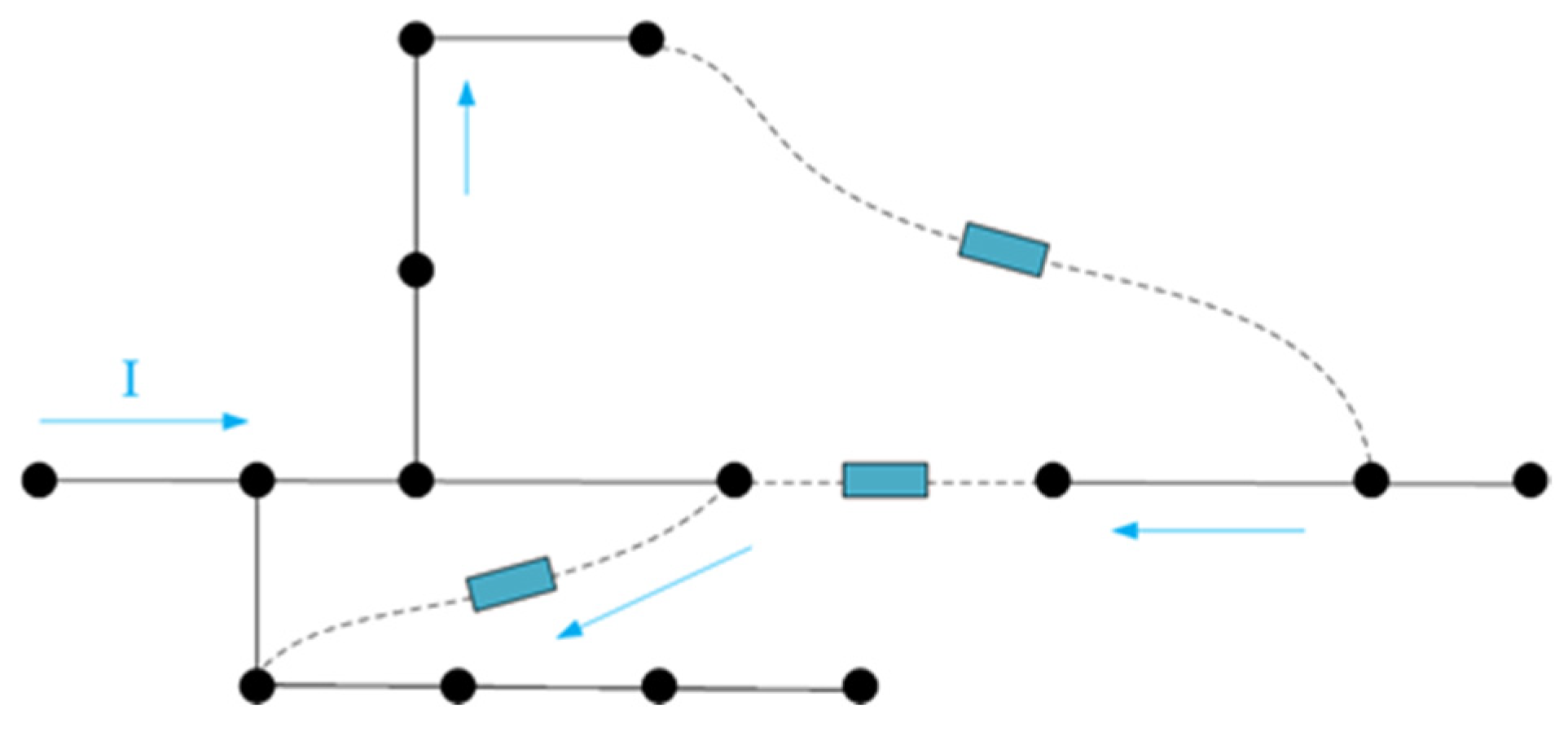
2.3. Model of Distribution Network Reconfiguration

Distribution network reconfiguration involves using computer and communication technologies to operate the line switches and tie switches within the distribution network. This is performed to either open or close these switches, thereby achieving optimal current flow distribution. The goal is to minimize network losses or balance the line loads, as illustrated in Figure 3. In Figure 3, the black dots represent the electrical system network nodes, while the cyan rectangles symbolize the line switches or tie switches. By altering the network topology, it is possible to reduce the energy losses during current transmission, thereby enhancing the overall efficiency of the distribution network.

In the reconfiguration of distribution networks, the objective function typically focuses on minimizing network losses. This is achieved by adjusting the status of switches within set Ω_b to alter the network topology of the distribution grid, as described in (3) and (4).

$$\min {\displaystyle \sum _{(ij)\in {\Omega }_b}{R}_{ij}{I}_{ij}^2}$$

(3)

$$I_{ij}^2={\displaystyle \frac{P_{ij}^2+Q_{ij}^2}{V_i^2}}$$

(4)

where Ω_b are all branches of the distribution network; R_ij is the resistance of the branch ij; I_ij is the magnitude of the current flowing through the branch ij; P_ij and Q_ij are the active and reactive power at the first node of the branch ij, respectively; V_i is the magnitude of node i voltage.

In the distribution network reconfiguration model, switches can only exist in two states: closed or open, which can be represented by 0 and 1, respectively. Therefore, the switch control variable is a discrete variable, possessing only two states: 0 and 1. If there are M switches within a distribution network, the entire system can potentially assume 2^M different states of these variables.

2.4. Model of Energy Storage

Currently, the most commonly used energy storage devices are electrochemical batteries. The output model of electrochemical energy storage can be represented by (5), where SOC stands for the DG. This SOC changes as the battery charges and discharges.

$$\begin{array}{l}SO{C}_t=\left\{\begin{array}{l}(1-d)\cdot SO{C}_{t-1}+{\displaystyle \frac{P_{c,t}{\eta }_c}{E_{bess}}}\Delta t, \mathrm{charging}\\ (1-d)\cdot SO{C}_{t-1}-{\displaystyle \frac{P_{d,t}}{{\eta }_d{E}_{bess}}}\Delta t, \mathrm{discharging}\end{array}\right.\\ \end{array}$$

(5)

where SOC_t and SOC_t−1 are the charge storage states of the energy storage device battery at moments t and t − 1, respectively; d is charging and discharging rate; η_c and η_d are the charging and discharging efficiency of energy storage. E_bess is the rated capacity of the energy storage. P_c,t and P_d,t are charging and discharging power of the battery at moment t.

To extend the service life of the energy storage device batteries, during the charging and discharging process, the battery’s SOC, charging and discharging power, and battery capacity must satisfy the constraints expressed in (6) to (8).

$$SO{C}_{\mathit{min}}\le SO{C}_t\le SO{C}_{\mathit{max}}$$

(6)

$$0\le P_{c,t}\le P_{cmax}$$

(7)

$$0\le P_{d,t}\le P_{dmax}$$

(8)

where P_c,t > 0 indicates that the battery is charging; P_d,t > 0 indicates that the battery is discharging; SOC_t indicates the capacity of the battery at time t; SOC_max and SOC_min indicates the upper and lower limits of battery capacity; P_cmax and P_dmax indicates the maximum charging power and maximum discharging power of the battery, respectively.

Since the battery charging and discharging states are mutually exclusive at the same moment, the battery charging and discharging powers P_c,t and P_d,t satisfy the following constraints.

$$P_{c,t}\cdot P_{d,t}=0$$

(9)

Energy storage devices can dispatch loads or power sources, charge during periods of low electricity prices, discharge during periods of high prices to achieve arbitrage, and optimize economic benefits. B₁ represents the profit of the energy storage device from “low storage high release” within a day.

$$B_1=-{\displaystyle \sum _{t=1}^{24}[P_{c,t}\cdot Y_{ch,t}\cdot {\lambda }_{c,t}-P_{d,t}\cdot Y_{dis,t}\cdot {\lambda }_{dis,t}]}$$

(10)

where t is a moment in the day; when the stored energy is charging at moment t, Y_ch,t = 1, Y_dis,t = 0; when the stored energy is discharging at moment t, Y_ch,t = 0, Y_dis,t = 1; λ_c,t is the charging tariff for energy storage at moment t; λ_dis,t is the discharge tariff of the energy storage at moment t.

2.5. Model of Loads

2.5.1. Model of Electric Car

Electric vehicle charging load is influenced by battery parameters, travel patterns, charging modes, and charging pile configuration. Charging station loads need to take into account the number of vehicles, types, charging modes, time periods, and starting power. The operation mode and tariff policy also affect the load distribution. In this paper, we focus on private car load clusters, whose driving routes and times are fixed, and whose charging moments and mileage are normally distributed [16,17]. The probability density function of private car start charging moment t_s can be expressed as (11).

$$f_T(t_s)=\left\{\begin{array}{l}{\displaystyle \frac{1}{\sqrt{2\pi }{\sigma }_s}}\exp \left({\displaystyle \frac{{(t_s-{\mu }_s)}^2}{2{\sigma }_s^2}}\right),\hspace{1em}({\mu }_s-12)<t_s<24\\ {\displaystyle \frac{1}{\sqrt{2\pi }{\sigma }_{\mathrm{s}}}}\exp \left({\displaystyle \frac{{(t_s+24-{\mu }_s)}^2}{2{\sigma }_s^2}}\right),\hspace{1em}0<t_s<({\mu }_s-12)\end{array}\right.$$

(11)

where μ_s is the expected value of the final arrival moment of the electric vehicle; σ_s is its standard deviation; the expression for the probability density function obeyed by the electric vehicle daily mileage s is expressed in (12).

$$f_D(s)=\left\{{\displaystyle \frac{1}{s{\sigma }_D\sqrt{2\pi }}}\exp \left(-{\displaystyle \frac{{(\ln s-{\mu }_D)}^2}{2{\sigma }_D^2}}\right)\right.$$

(12)

where μ_D is the expected daily driving range of an electric vehicle; σ_D is its standard deviation; the computational expression for the electric vehicle charging duration t_ch is expressed in (13).

$$t_{ch}={\displaystyle \frac{s{W}_{100}}{100{\eta }_c{P}_c}}$$

(13)

where W₁₀₀ indicates the 100-km power consumption of electric vehicles; s indicates the daily mileage of electric vehicles; η_c, P_c denote charging efficiency and charging power, respectively.

The probability that the electric car is charging at moment t is expressed in (14).

$$F_{ch}(t)={\displaystyle {\int }_0^{t_{chmax}}{\displaystyle {\int }_0^{t-t_{ch}}{f}_{tch}{f}_{T}d{t}_{s}d{t}_c+{\displaystyle {\int }_0^{t_{chmax}}{\displaystyle {\int }_t^{t+24-t_{ch}}{f}_{tch}{f}_{T}d{t}_{s}d{t}_c}}}}$$

(14)

where f_tch is the probability density function of electric vehicle charging duration; t_chmax is the maximum value of the charging duration.

This paper is based on Monte Carlo stochastic sampling to portray the scaled electric vehicle charging load profile. Monte Carlo sampling is a stochastic simulation sampling method, which uses probability and statistical theories, establishes probabilistic models, and performs sampling simulation with the help of computers to calculate the approximate solution of electric vehicle charging demand.

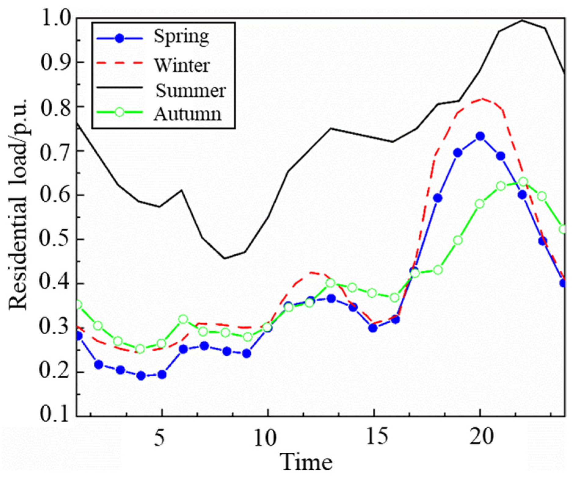
2.5.2. Model of Load Power

In this paper, only residential and commercial loads are considered in the model for the actual situation of the distribution network. Based on the analysis of historical electricity load data from residential and commercial sectors in a specific region, this study developed a load time-series forecasting model. Through this model, characteristic load curves for typical days across four seasons were simulated for both residential and commercial loads, as shown in Figure 4 and Figure 5.

From Figure 4 and Figure 5, it can be seen that because of the differences in the nature of the loads, there are large differences in the timing characteristics of residential loads and commercial loads: residential loads reach their highest loads in summer, while commercial loads have a small difference in the timing characteristics of electricity consumption in different seasons.

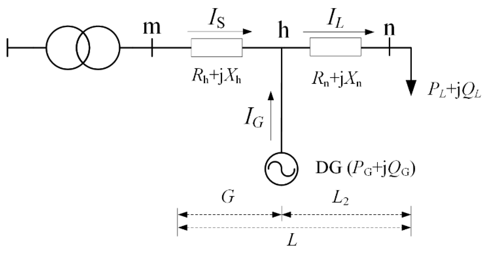
3. Analysis of Factors Affecting Network Losses in Distribution Networks

For an active distribution network incorporating DG, it is assumed that the load is connected in a Y configuration and maintains three-phase balance with a constant power factor, absorbing both active and reactive power from the grid. Additionally, the transmission line lengths are relatively short, allowing for the neglect of line-to-ground admittance, and the voltage variations along the transmission lines are minimal following the integration of DG [18,19]. The analysis of network losses in this idealized distribution system after DG integration is depicted in Figure 6.

After accessing DG (P_G + jQ_G) at node h in the middle of the line, at this time, the network loss is divided into two parts to be calculated: the first half of the line network loss between the substation to the DG P_loss1 and the second half of the line network loss between the DG to the end of the line P_loss2. From Figure 6, it can be seen that, at this time, the inflow of the load of the single-phase current is expressed in (15).

$$I_L=I_S+I_G$$

(15)

where I_L is the load current; I_S is the supply current; I_G is the injection current of the DG.

Therefore, the net loss P_loss1 and P_loss2 can be expressed as (16) and (17).

$$\begin{array}{l}{P}_{loss1}=3rG{I_S}^2\\ \hspace{1em} ={\displaystyle \frac{rG(P_L^2+Q_L^2+P_G^2+Q_G^2-2P_L{Q}_L-2P_G{Q}_G)}{3U^2}}\end{array}$$

(16)

$$P_{loss2}=3r(L-G){I_L}^2={\displaystyle \frac{r(L-G)(P_L^2+Q_L^2)}{3U^2}}$$

(17)

where G is the length of the line from node m at the head of the line to node h at the DG installation.

From (16) and (17), the network loss P_loss1 and P_loss2 are obtained, and the total line loss after accessing the DG can be obtained by summing the two.

$$\begin{array}{l}{P}_{loss}=P_{loss1}+P_{loss2}\\ \hspace{1em} ={\displaystyle \frac{rL}{3U^2}}[P_L^2+Q_L^2\\ \hspace{1em} +(P_G^2+Q_G^2-2P_L{Q}_L-2P_G{Q}_G)({\displaystyle \frac{G}{L}})]\end{array}$$

(18)

Deriving for DG capacity P_G and Q_G, the sensitivity of AC loss P_loss to DG active and reactive power is deduced.

The effect of change in DG active reactive capacity on AC loss is expressed in (19) and (20).

$$LSF{P}_t={\displaystyle \frac{\partial P_{loss}}{\partial P_G}}={\displaystyle \frac{2rG}{3U^2}}\left(2P_G-Q_G\right)$$

(19)

$$LSF{Q}_t={\displaystyle \frac{\partial P_{loss}}{\partial Q_G}}={\displaystyle \frac{2rG}{3U^2}}\left(Q_G-P_G\right)$$

(20)

where LSFP_t and LSFQ_t denote the sensitivity of DG active and reactive power to affect network losses, respectively.

From (19) and (20), it can be seen that the active power injected by the DG has a greater impact on the network loss sensitivity than the reactive power. The siting and capacity of distributed PV are related to the network loss, while the actual power variation has a large randomness, and it is difficult to accurately calculate the network loss using deterministic methods. Therefore, this paper adopts the Latin hypercubic sampling algorithm, which can effectively assess the network loss.

4. Improved Particle Swarm Optimization Algorithm

4.1. Conventional Particle Swarm Optimization Algorithm

In this paper, the particle swarm optimization (PSO) algorithm is employed to address bi-level programming problems [20]. The PSO algorithm is an evolutionary computation technique that simulates the foraging behavior of bird flocks. It conceptualizes solutions within the problem space as the distribution of individual positions within a flock during foraging. Through the transmission of information among individuals, the algorithm drives the entire population toward areas of potential food sources, thereby progressively increasing the likelihood of identifying optimal solutions. In this algorithm, the updates of particle positions and velocities are as follows:

$$v_{i,j}^{k+1}=w{v}_{i,j}^k+c_1{r}_1\left(p_{i,j}^k-y_{i,j}^k\right)+c_2{r}_2\left(g_{i,j}^k-y_{i,j}^k\right)$$

(21)

$$y_{i,j}^{k+1}=y_{i,j}^k+v_{i,j}^{k+1}$$

(22)

where i is the number of particles; j is the dimensionality of variables; c₁ and c₂ are learning factors; $v_{i,j}^k$ is the velocity of the i-th particle in the j-th dimension during the k-th generation; $y_{i,j}^k$ is the position of the i-th particle in the j-th dimension at the k-th iteration.

4.2. Improved PSO

With regard to the limitations of the PSO algorithm, such as low convergence precision and susceptibility to local optima entrapment, numerous scholars have conducted research and proposed various improvement methods [21,22]. Through adjustments to population initialization, inertia weight, learning factor optimization, and boundary constraint handling, an improved PSO algorithm has been developed [23].

In view of the excellent convergence performance of the improved PSO algorithm, this paper mainly adjusts the inertia weights and evolution strategy based on it.

4.2.1. Population Initialization

This paper employs chaotic mapping for initialization. Compared to random initialization, chaotic mapping can generate sequences that are neither periodic nor convergent. When these sequences are mapped back to the solution space, they can enhance population diversity, thereby improving search capability and preventing premature convergence. Equations (23) and (24), which use a sine function to generate chaotic variables, demonstrate superior chaotic characteristics.

$$\left\{\begin{array}{l}{x}_j^{n+1}=1.18\cdot \sin {\displaystyle \frac{2}{x_j^n}}, -1\le x_j^n\le 1, x_j^n\ne 0\\ y_j^{n+1}=1.18\cdot \sin {\displaystyle \frac{2}{y_j^n}}, -1\le y_j^n\le 1, y_j^n\ne 0\end{array}\right.$$

(23)

$$\left\{\begin{array}{l}{x}_{ij}={\displaystyle \frac{(x_j^n+1)\cdot (x_{max}(j)-x_{min}(j))}{2}}+x_{min}(j)\\ y_{ij}={\displaystyle \frac{(y_j^n+1)\cdot (v_{max}(j)-v_{min}(j))}{2}}+v_{min}(j)\end{array}\right.$$

(24)

where $x_j^n$ and $y_j^n$ represent chaotic variables with different initial values; x_max(j) and x_min(j) represent the maximum and minimum values of the particle’s position in the jth dimension; v_max(j) and v_min(j) represent the maximum and minimum values of the particle’s velocity in the jth dimension.

4.2.2. Adaptive Inertia Weight

The adjustment of inertia weight has traditionally evolved from fixed values to a linear decrease and even a nonlinear decrease, which, to some extent, simulates the need for complexity and dynamic changes in the optimization process. This paper introduces an adjustable directional component, allowing the inertia weight not only to decrease with increasing iterations but also to adjust more flexibly according to the actual performance and requirements during the search process, as shown in (25) and (26).

$$w(i)=w_{max}-(w_{max}-w_{min})\cdot ({\displaystyle \frac{t}{T}})^q(i)$$

(25)

$$q(i)=1.8+2\cdot ({\displaystyle \frac{ac\tan (\log \frac{fit-pbest(i)}{fit-mean})}{\pi }})$$

(26)

where w_max and w_min represent the maximum and minimum values of inertia weights, respectively; T represents the total number of iterations; q(i) represents the index factor, which is used to describe the trend of the inertia weight magnitude of the ith particle as it updates its position in the same generation; fit-pbest(i) represents the fitness value of the ith particle; fit-mean represents the average fitness value of all individual particles in the population.

When the fitness value of the particles is high, this strategy makes the inertia weights adjusted in the direction of w_max to enhance the global search ability; on the contrary, when the fitness value is low, the inertia weights will be adjusted in the direction of w_min to improve the local search accuracy [24]. This strategy not only enhances the algorithm’s ability to search in regions of high fitness but also promotes more efficient and accurate solution discovery.

4.2.3. Update the Velocity and Position of the Particles

In this paper, a heron hunting strategy is introduced into the particle swarm algorithm. In order to improve the optimization accuracy of the algorithm in the final stage of hunting, when the number of iterations t exceeds the preset threshold, the weighted Levy flight strategy is used for optimization, and its equations are shown in (27) and (28).

$$\left\{\begin{array}{l}{v}_i^j(t+1)=w(I)\cdot v_i^j(t)+C_1\cdot \mu \cdot (p_i^j(t)-x_i^j(t))+C_2\cdot \mu \cdot (g^j(t)-x_i^j(t))\\ x_{i+1}^j(t+1)=x_i^j(t)+\varphi \cdot v_i^j(t+1)\end{array}\right.$$

(27)

$$\left\{\begin{array}{ll}\varphi =1,& t\le {\displaystyle \frac{2}{3}}T\\ \varphi =0.5\cdot Levy(D),& t>{\displaystyle \frac{2}{3}}T\end{array}\right.$$

(28)

where Levy(D) is the Levy flight distribution function; the other parameters are as previously defined.

4.2.4. Treatment of Border Crossings

In this paper, the stochastic reset method is used to generate new values for variables randomly within the allowed range. This method effectively increases the diversity of the population and helps to prevent the algorithm from prematurely converging to a local optimal solution, which is handled as shown in (29).

$$\left\{\begin{array}{l}{x}_i^j=x_{max}(j)-\mu (x_{max}(j)-x_{min}(j))\\ v_i^j=v_{max}(j)-\mu (v_{max}(j)-v_{min}(j))\end{array}\right.$$

(29)

5. Loss Reduction in Distribution Networks with “Source-Network-Hoist-Storage” Coordination

5.1. Analysis of Loss Reduction Strategies for Distribution Network Losses

This paper discusses the impacts of DG, energy storage, and electric vehicle charging loads on renewable energy consumption and network losses in distribution networks and proposes a coordinated optimization strategy for the four links of “source-network-storage-load”. The coordinated optimization strategy diagram is shown in Figure 7.

Source side: Planning distributed PV siting and capacity and taking into account the uncertainty of light intensity to improve the accuracy of planning.

Network side: Reconfigure the distribution network to achieve a local balance of DG output and even distribution of loads and reduce network losses.

Storage side: Planning the capacity and location of energy storage devices, participating in the coordinated operation of the grid, enhancing renewable energy consumption, and reducing losses.

Load side: Guiding the orderly use of electricity through time-sharing tariffs, shaving peaks and filling valleys, reducing equipment losses, and improving economy.

5.2. The Coordinated Bi-Level Optimization Model of Source–Grid–Load–Storage

This section aims to enhance the consumption of renewable energy, reduce network losses, stabilize voltage, and decrease costs through optimizing the operational output of PV systems and energy storage and by guiding electric vehicle charging. The loss in the distribution network is closely related to the siting and sizing of distributed source–storage, which pertains to a planning issue. The stochastic nature of PVs and electric vehicles affects power flow and, consequently, leads to losses, which is an operational issue. Therefore, this paper employs a bi-level planning model that integrates planning and operational optimization to improve the consumption of renewable energy and reduce grid losses.

The bi-level optimization problem comprises two hierarchical optimization models. The lower-level optimization is conducted under the parameters and constraints set by the upper-level decision-maker. The upper-level optimization, in turn, modifies the decision variables based on the results from the lower level, thereby completing the optimization process. This model is represented as (30).

$$\left\{\begin{array}{c}\min F=F(x,w)\\ \mathrm{s}.\mathrm{t}.\begin{array}{c}\end{array}G(x)\le 0\\ \min w=f(x,y)\\ \mathrm{s}.\mathrm{t}.\begin{array}{c}\end{array}g(x,y)\le 0\end{array}\right.$$

(30)

where F(∙) is the objective function of the upper level; w(∙) is the objective function of the lower level; G(∙) is the constraints associated with the upper-level objective function; g(∙) is the constraints of the lower-level objective function; the decision variable x is the upper-level objective; y is the decision variable for the lower-level objective.

This paper establishes a bi-level optimization model to reduce losses in the distribution network. The upper-level model aims to minimize the total cost by determining the location and capacity of energy storage stations. The lower-level model focuses on minimizing load fluctuations, optimizing node voltages, and maximizing the consumption of PV energy. It considers the output from energy storage and PV systems and the charging strategies for electric vehicles. The schematic diagram of the bi-level optimization model is shown in Figure 8.

5.2.1. Upper-Level Planning Mathematical Model

The objective function for the upper-level planning model is set to minimize the annual total planning cost of the system [25]. The planning costs of the system typically comprise three main components: the investment costs; operation and maintenance costs of distributed PV systems, energy storage systems, and electric vehicle charging stations; and the cost of electricity purchased from the main grid [26]. The decision variables for the upper-level planning include the locations and capacities of two PV power sources, two energy storage systems, and two electric vehicle charging stations. The objective function is represented as (31).

$$f_1=\alpha C_{inv}+C_{ope}+C_{en}$$

(31)

where C_inv is the total investment cost; C_ope is the system’s operation and maintenance costs; C_en is the cost of purchasing electricity for the system; α is the annual equivalent coefficient. the expression for which is as follows.

$$\alpha ={\displaystyle \frac{r{\left(1+r\right)}^{LT}}{{\left(1+r\right)}^{LT}-1}}$$

(32)

where r is the discount rate; LT is the lifetime of the equipment.

The constraints of the upper-level planning mathematical model are mainly a series of constraints and inequality constraints as follows.

(1)

Capacity constraints for distributed PV power.

The main constraints include that the capacity of the distributed PV sources at each node should be less than their maximum capacity. Additionally, the total capacity of all DG units must be less than the capacity of the load nodes.

$${\displaystyle \sum _{s\in {\Omega }_1}{P}_{s,j}^{PV}\le \eta {\displaystyle \sum _{s\in {\Omega }_1}{\displaystyle \sum _{i=1}^n{P}_{s,i}^L}}}$$

(33)

where η is PV power factor; $P_{s,j}^{PV}$ is the access capacity for distributed PV power; $P_{s,i}^L$ is the node i load power; n represents all load nodes.

(2)

The constraints on the installed capacity, charging and discharging efficiency, and state of charge of the energy storage system are given in (5) to (9).

(3)

Power balance constraints in the distribution system.

$$P_t^{PV}+P_t^{bess}+P_t^l=P_t^{load}+P_t^{loss}$$

(34)

$$P_t^{loss}={\displaystyle \sum _{k=1}^{N_L}{P}_{t.k}^{loss}}$$

(35)

where P_t^PV is the active power of the PV at time t; P_t^bess is the active power of the stored energy at time t; P_t^l is the contact line conveying power at time t; P_t^load is the load power at time t; P_t^loss is the active losses in the system at time t; P_t._k^loss is the active loss of branch k at time t.

(4)

Contact line power constraint.

$$0\le P_k\le P_k^{\max }$$

(36)

That is, the power allowed to pass through any kth branch does not exceed the maximum power allowed to pass through that branch.

5.2.2. Lower-Level Planning Mathematical Model

The lower level of the model is designated as the operational dispatch layer, with its objective functions aiming to minimize the variance of the load curve in the distribution system and the voltage deviation at the nodes.

$$\min f_1={\displaystyle \frac{1}{T}}{\displaystyle \sum _{t=1}^T\left(P_{L,t}-\frac{1}{T}{\displaystyle \sum _{t=1}^T{P}_{L,t}}\right)}$$

(37)

$$\min f_2={\displaystyle \sum _{i=1}^{N_{bus}}{(u_i-u_N)}^2}$$

(38)

where P_L,t is the net load power of the load distribution network; T is the operating period of a day; u_i is the actual voltage at node i; u_N is the rated voltage of the distribution network.

For ease of solution, it is assumed that the lower bi-objective function is reduced to a single objective function.

$$F=\lambda f_1+\theta f_2$$

(39)

where λ and θ are the objective function coefficients, respectively, indicating the weights occupied by f₁ and f₂ to the comprehensive objective function F. The sum of the two is 1. By adjusting the changes in λ and θ, the objective function under different weights can be optimized. At this time, the lower objective function can be written as (40).

$$\min F=\lambda f_1+\theta f_2$$

(40)

Constraints are included:

(1)

Electric power flow constraints.

$$\begin{array}{l}{P}_i=U_i{\displaystyle \sum _{j\in i}{U}_j(G_{ij}\cos {\theta }_{ij}+B_{ij}\sin {\theta }_{ij})}\\ Q_i=U_i{\displaystyle \sum _{j\in i}{U}_j(G_{ij}\sin {\theta }_{ij}-B_{ij}\cos {\theta }_{ij})}\end{array}$$

(41)

(2)

Distributed PV power supply, energy storage system output constraints, node voltage constraints, and line power constraints.

$$P_{PV}^{max}(t)=P_{PV}(t)\times P_{Cap}^{PV}$$

(42)

$$0\le P_{PV}(\mathrm{t})\le P_{PV}^{max}(t)$$

(43)

$$0\le P_{c,t},P_{d,t}\le P_{Cap}^{ESS}$$

(44)

$${U_i}^{min}\le U_i\le {U_i}^{max}$$

(45)

$$S_{Li}\le S_{Lmax}$$

(46)

where $P_{PV}^{max}(t)$ is the maximum PV output at moment t; P_PV(t) is the actual output of PVs at moment t; $P_{Cap}^{ESS}$ is the maximum power limit for energy storage charging and discharging; S_Li is the apparent power of line i.

5.3. Model Solving Method

The flowchart of the model solving step is shown in Figure 9.

Step 1: Input PSO algorithm parameters, system parameters, and corresponding constraints.

Step 2: Optimize the site selection of the distributed power supply.

Step 3: Set the location and corresponding initial capacity of distributed PV and energy storage installation, initialize the upper particle swarm, and take the installed capacity of the energy storage device and distributed PV as particles.

Step 4: Based on the capacity of distributed PV obtained by solving, the output of PV in each seasonal scenario can be obtained; begin the particle swarm algorithm population initialization process.

Step 5: Solve the lower-level model to optimize the capacity of the charging station of the energy storage system, and then obtain the value of the lower-level objective function and the optimal output of the storage system and the charging station at each moment.

Step 6: Return the values from step 5 and solve the upper-layer model subject to the constraints.

Step 7: Update the upper-layer PSO model to produce a new particle swarm.

Step 8: Determine whether the set number of iterations is reached; if so, the program run ends; otherwise, execute step 4 and go to the next iteration.

6. Case Study

6.1. Parameters of Case

In this paper, IEEE 33-node arithmetic is used to simulate the distribution network, as shown in Figure 10. The topology of the distribution network is radial, with power flowing unidirectionally from the substation to end users. The maximum total load of the distribution network is 3.41 MW + 1.02 Mvar, the rated voltage is 12.66 kV, the permissible range of the node voltage is 0.95~1.05 p.u., and the maximum penetration rate of PV does not exceed 30%. The model contains two PV power sources, two energy storage systems, and two electric vehicle charging stations, taking into account the correlation of light intensity between PV power stations and timing characteristics. The charging loads are guided according to the previous method and the introduction of time-of-day tariff curves. Figure 11 shows the time-of-use electricity price curve, with electricity prices reaching daily peaks during the period from 14:00 to 16:00 in the afternoon, assuming that the tariffs are the same in all seasons. The load model is based on commercial and residential electricity consumption, with weights of 55.8% and 44.2%, respectively, and the typical days of the four seasons are used to represent the annual load curve, with the number of days in spring, summer, autumn, and winter being 91, 90, 91, and 93, respectively. The MATPOWER 7.1 extension package is used to perform the power flow calculations and determine network losses.

6.2. The Role of “Source-Grid-Load-Storage” Coordination on Distribution Network Loss Reduction

The maximum number of iterations set for the model is 400; the number of particle swarms is 100; the dimensions of the decision variables are 108, including the 24 h outputs of two PV power sources, two energy storage power stations, and the locations and capacities of them and the EV charging stations, with the upper and lower weights of 0.9 and 0.4, respectively; and the upper speed limit of maximum is 10. Figure 12 shows the iterative convergence diagram of this two-layer optimization model, and the curves in the diagram indicate that the model has good convergence and the optimization results tend to be stable after 300 iterations.

Table 1. Optimal configuration of photovoltaic systems, energy storage, and electric vehicles for situation 6.

Photovoltaic (kW)	Energy Storage (kWh)	Electric Vehicle (kW)
Node 18: 381.1 (400)	Node 6: 517.5 (500)	Node 1: 259.1 (250)
Node 24: 200.1 (200)	Node 13: 537.9 (500)	Node 20: 247.5 (250)

demonstrates the optimal configuration of capacity for PV, storage, and electric vehicles, rounded to the actual installed capacity. This configuration results in a renewable energy penetration of 17.6 percent, with electric vehicles accounting for 14.7 percent and energy storage accounting for 29.3 percent. Figure 13, Figure 14, Figure 15, Figure 16 and Figure 17 show the results of the model solution under situation 6 at the moment of 12:00, comparing the voltage distribution at the IEEE 33-node of the distribution network before and after the optimization. After optimization, the voltage of all nodes is increased, especially the nodes far away from the main node, e.g., the voltage of node 18 is increased from 0.946 to 0.984, which is an increase of 4.6%, and the voltage of all nodes is more than 0.95, which meets the requirements of the distribution network.

Figure 14 shows the change in network losses of the distribution network before and after the co-optimization of PV, storage, and electric vehicles. The original distribution network nearly doubles at 20 o’clock due to the surge in network losses caused by electric vehicle charging. After the optimization, the network loss is generally reduced, especially the peak loss at the 20 o’clock moment, which decreases by 53.6%, and only the loss at the 4, 5, and 6 moments is slightly higher or close to the original load loss. Based on the analysis of network loss data across 24 hourly time sections, the overall network loss after optimization showed a significant reduction of approximately 37.2% compared to pre-optimization levels, thoroughly demonstrating the efficiency and practical value of this optimization strategy in reducing power grid energy consumption.

Figure 15 shows the 24 h operation plan of the two energy storage systems, with maximum charging and discharging power of 302.3 kW and 309.5 kW for storage 1 and 374.5 kW and 393.7 kW for storage 2. The energy storage system discharges during peak loads and charges during troughs, thus smoothing the load power curve and realizing the “peak shaving” and “valley filling” principle. The energy storage system discharges at peak loads and charges at troughs to flatten the load power curve and achieve “peak shaving and valley filling”. As shown in Figure 16, the energy storage system is charged at a time of low electricity prices and discharged at a time of peak electricity prices, making full use of the “low storage and high generation” characteristics of the energy storage device and following the order of charging first and then discharging.

After connecting to the electric vehicle, the community load increases and fluctuates, especially at 20 o’clock. The charging and discharging of the energy storage system flattens the load peaks and valleys and boosts the valleys so that the maximum load is close to the original load. Figure 17 shows the distributed PV power curve, which has a shortfall and abandonment in the PV power plan due to the contradiction between the PV O&M cost in the objective function and the voltage quality and abandonment penalty function. PV power supply 1 is at full power, PV power supply 2 does not have enough power, and the rate of abandoned light reaches 26.9%, which does not achieve the maximum consumption of renewable energy.

6.3. Rationality and Effectiveness Analysis

In order to understand and verify the reasonableness and validity of the model, the following six scenarios are selected to compare the economic benefits and network losses.

Situation 1: The scenario without considering distributed PV, energy storage, and EV access.

Situation 2: Considering only the role of energy storage devices.

Situation 3: Only distributed PV access is considered.

Situation 4: Considering only electric vehicle access.

Situation 5: Consider both distributed PV and electric vehicle access.

Situation 6: Distributed PV, energy storage device, and electric vehicle are all connected to the case.

Situation 1 is the original load with no DG, storage, and electric vehicle access, and the network loss cost is CNY 1,175,000. In situation 2, with the addition of storage, the network loss cost is reduced to CNY 995,900, which is a reduction of 18%, the cost of purchased power is reduced by CNY 864,000, the arbitrage of energy storage is realized at CNY 836,000, and the total consumption is increased by CNY 401,000. After situation 3 connects to PV, the cost of purchased power decreases from CNY 20,597,000 to CNY 19,904,000, and the network loss decreases by CNY 197,400. After connecting to EVs in situation 4, the network loss increases by CNY 42,800, and the cost of purchased electricity increases by CNY 1,316,000. Situation 5 connects to both PV and electric vehicles, with a net loss cost of CNY 981,700 and a purchased power cost of CNY 21,254,000. In situation 6, co-optimization reduces network losses to CNY 844,000, a reduction of 39.2%, and purchased power costs of CNY 20,141,000, for a total cost of CNY 22,947,000, which is an increase of CNY 1,175,000 compared to situation 1 but saves more compared to situations 4 and 5. After co-optimization, PV output is maximized, and storage shifts load and reduces imbalance, with no significant increase in the total cost, providing a strategy for distribution network planning. The introduction of distributed power, storage, and EVs increases costs, but the total costs after co-optimization only increase by 5.4% compared to situation 1, before government subsidies.

Figure 18 shows the configured capacity of distributed PV, energy storage, and electric vehicles for the six situations. The storage system alone has the largest configured capacity, 604.12 kW and 662.46 kW, respectively, which is higher than the 517.5 kW and 537.9 kW of situation 6. The configured capacity of the PV and electric vehicle without storage is only 200 kW; the configured capacity of the PV and electric vehicle is increased by the coordinated configuration of storage, which indicates that the energy storage system is essential to increase the capacity of the PV and electric vehicle and is an indispensable part of the distributed power allocation, verifying the necessity of the “source-storage-load-grid” coordinated optimization. This shows that the energy storage system is essential for improving the consumption capacity of PV and electric vehicles and is an indispensable part of the distributed power supply configuration, which verifies the necessity of the collaborative optimization of “source-storage-load-network”.

After the access of the energy storage system, the load curve fluctuation variance of the distribution network is reduced from 446.99 to 148.9, which significantly reduces the load volatility. Figure 19 demonstrates the load profile before and after situation 2 is added to the energy storage system. Figure 20 demonstrates the power output of the energy storage system in situation 2, and the comparison with the power curve in Figure 19 shows that the energy storage system presents obvious low-absorption and high-discharge characteristics; compared with the four synergistic optimizations, the energy storage power output characteristics are more prominent.

Figure 21 summarizes the load curve fluctuation variance, 24 h voltage deviation of all nodes, and annual network loss data across six scenarios. In situation 1, the original load curve fluctuation variance is 446.99, which decreases to 148.89 in situation 2 after the integration of the energy storage system, indicating that energy storage can effectively smooth load fluctuations. After the integration of PV power sources, the voltage at distribution network nodes improves, surpassing that of the standalone energy storage system. Following the coordinated optimization of PVs and energy storage, the load curve fluctuation variance and voltage deviation drop to 351.09 and 21.98, respectively, achieving the best results among the six situations.

After the coordinated optimization of PV and energy storage output, the network line losses were reduced to 1406.67 MWh, saving a cost of CNY 311,000 in network loss. The load curve fluctuation and voltage quality improved by 21.45% and 27.8%, respectively. The system consumed 1347.6 MWh of distributed PV energy per year and supplied 2002.1 MWh to electric vehicle loads. The results demonstrate that the “source-storage-load” coordinated optimization strategy effectively reduces the losses in active distribution networks, providing an important modeling tool for the construction and planning of modern distribution networks, with significant practical implications and application value.

To further validate the effectiveness and superiority of the proposed method, this paper compares the improved PSO with the traditional PSO, the genetic algorithm (GA), and the seagull optimization algorithm (SOA), as shown in

Table 2. Comparison of optimization algorithms.

Algorithm	Minimum Fitness Value	Number of Iterations	Computation Time(s)
Improved PSO	0.603	289	19.65
PSO	0.712	472	29.08
GA	0.725	392	28.66
SOA	0.734	413	34.75

. The data in the table demonstrates that the improved particle swarm algorithm has significant advantages in both solution quality and computational efficiency: the minimum fitness value is 0.603, notably lower than the other three algorithms; the iteration count is 289, considerably fewer than the 472 iterations required by traditional the PSO; and the computation time is only 19.65 s, significantly less than the 29.08 s for the traditional PSO, 28.66 s for the GA, and 34.75 s for the SOA. These results thoroughly demonstrate that the improved particle swarm optimization algorithm proposed in this paper provides higher solution accuracy and computational efficiency when solving the source–grid–load–storage coordinated optimization problem in distribution networks, offering a more efficient optimization tool for practical engineering applications.

In order to further validate the applicability and effectiveness of the proposed method in different sizes and types of power grids, the IEEE 118-node active distribution system and the DTU 7K 47-node real active distribution system are selected for testing and analysis in this paper, as shown in Figure 22 and Figure 23.

The IEEE 118-node active distribution network is a standard test system widely used to verify the accuracy and robustness of the algorithm. The network has a reference voltage of 12.6 kV and a reference power of 10 MVA, where node 52 is connected to a fourth-generation controllable wind turbine with a rated capacity of 1 MW. The actual load data from the Global Energy Forecasting Competition (GEFC) 2012 is used in this paper. The DTU 7K 47-node real active distribution network is a test system closer to the real application scenario. The system consists of three wind farms, all consisting of fourth-generation controllable turbines with an installed capacity of 12 MW, 15 MW, and 15 MW, respectively. The base voltage of the system is 10 kV, and the base capacity is 10 MVA.

Further optimization simulations (situation 6) were conducted on three test cases: the IEEE 33-node distribution system, the IEEE 118-node active distribution network, and the DTU 7K 47-node real active distribution network, each with coordinated integration of distributed photovoltaics, energy storage devices, and electric vehicles.

As shown in

Table 3. Comparison of different distribution network examples.

Distribution Network	Optimized Total Line Losses (MWh)	Savings in Network Loss Costs (CNY)
IEEE-33	1406.7	311,000
IEEE-118	4185.2	902,000
DTU	1828.7	429,000

, all test cases achieved significant reductions in network losses and improvements in economic benefits, verifying that the source–grid–load–storage coordinated optimization method proposed in this paper demonstrates good applicability across distribution networks of different scales and complexities.

7. Conclusions

Coordinating source–grid–load–storage resources to reduce network losses is crucial to the secure and economical operation of modern power systems. This paper constructs a bi-level optimization model for reducing power system losses. At the upper level, the model selects sites and sizes for distributed PV sources and energy storage systems. At the lower level, it controls the intraday operational output of the storage and PV stations to maximize PV integration, minimize network losses, improve system security levels, and smooth fluctuations in the load curve. By comparing the annual costs and network losses across six situations, the conclusions are as follows:

(1)

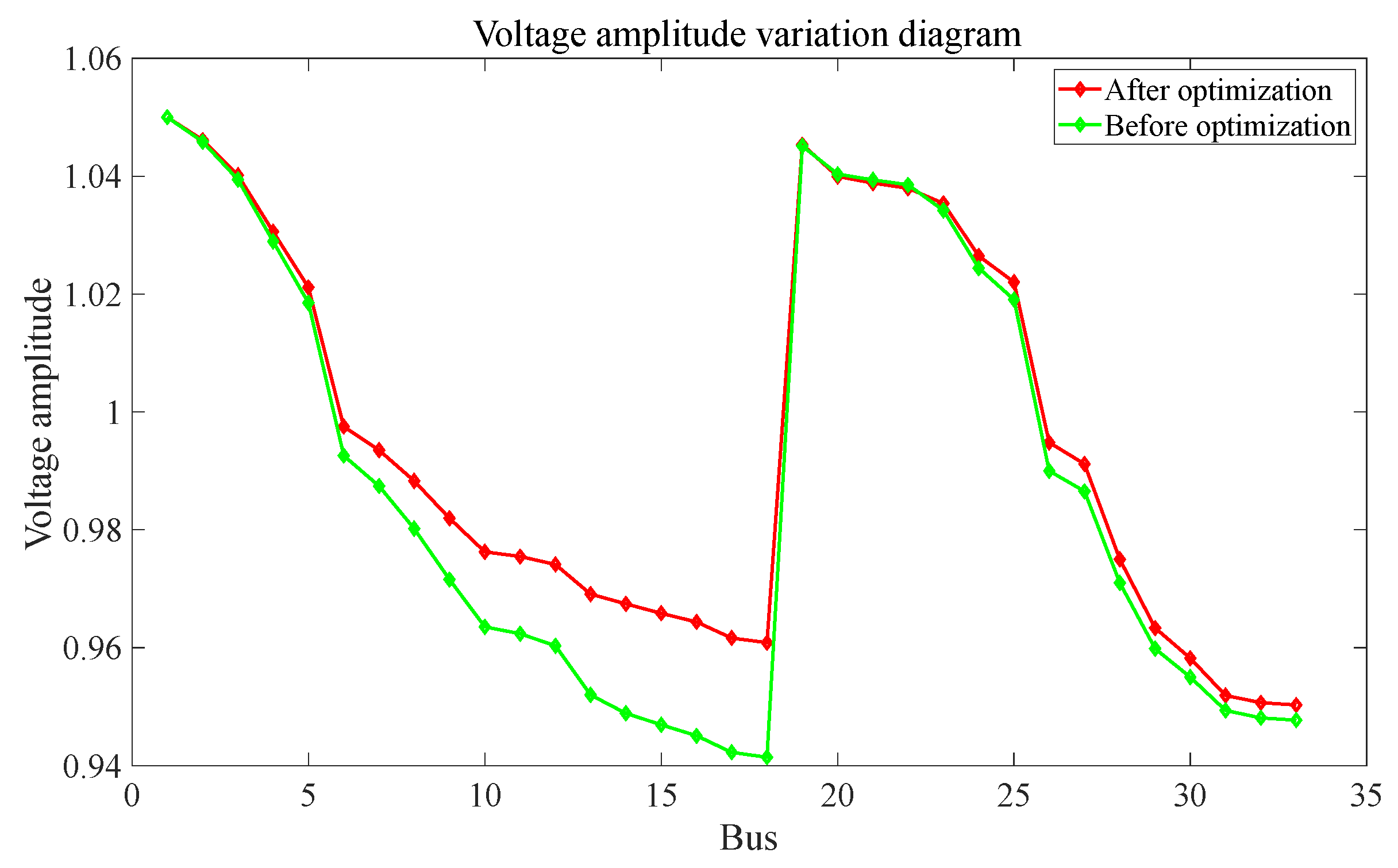
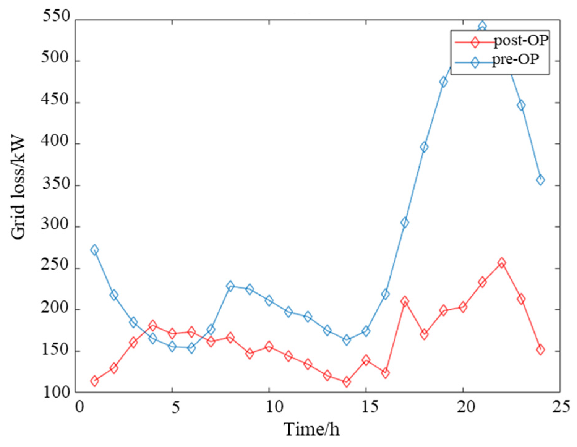
Integrating distributed PV power generation systems into the distribution network reduces network losses and annual power purchase costs; integrating energy storage systems into the distribution network decouples simultaneous load demands, reduces peak-to-valley differences in the load curve, and thus reduces network losses; coordinated optimization of source–storage–load maximizes the consumption of PV power generation, reduces network losses, improves the system security levels, and reduces the fluctuation of the load curve.

(2)

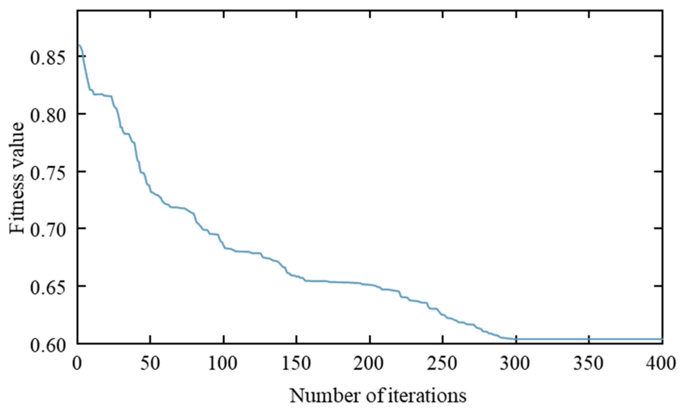
The improved particle swarm algorithm proposed in this paper outperforms the traditional algorithm in terms of minimum fitness value, number of iterations, and computation time, and it provides higher solution accuracy and computational efficiency for the distribution network coordination optimization problem.

(3)

Through the IEEE 33-node distribution network and the IEEE 118-node and DTU 7K 47-node systems, the proposed method shows good applicability in different sizes and types of distribution networks, which can significantly reduce network losses and improve economic efficiency.

Future research could consider exploring integrated optimization of various renewable energies, such as wind and biomass.

References

1. Tong, H.; Zeng, X.; Yu, K.; Zhou, Z. A Fault Identification Method for Animal Electric Shocks Considering Unstable Contact Situations in Low-Voltage Distribution Grids. IEEE Trans. Ind. Inform. 2025, 1–12. [Google Scholar] [CrossRef]
2. Yu, Y.; Guo, J.; Jin, Z. Optimal extreme random forest ensemble for active distribution network forecasting-aided state estima-tion based on maximum average energy concentration VMD state decomposition. Energies 2023, 16, 5659. [Google Scholar] [CrossRef]
3. Yu, Y.; Jin, Z.; Ćetenović, D.; Ding, L.; Levi, V.; Terzija, V. A robust distribution network state estimation method based on enhanced clustering Algo-rithm: Accounting for multiple DG output modes and data loss. Int. J. Electr. Power Energy Syst. 2024, 157, 109797. [Google Scholar] [CrossRef]
4. Cao, Y.; Zhou, B.; Chung, C.Y.; Wu, T.; Zheng, L.; Shuai, Z. A coordinated emergency response scheme for electricity and watershed networks con-sidering spatio-temporal heterogeneity and volatility of rainstorm disasters. IEEE Trans. Smart Grid 2024, 15, 3528–3541. [Google Scholar] [CrossRef]
5. Xia, Y.; Li, Z.; Xi, Y.; Wu, G.; Peng, W.; Mu, L. Accurate Fault Location Method for Multiple Faults in Transmission Networks Using Travelling Waves. IEEE Trans. Ind. Inform. 2024, 20, 8717–8728. [Google Scholar] [CrossRef]
6. Xu, Y.; Han, J.; Yin, Z.; Liu, Q.; Dai, C.; Ji, Z. Voltage and reactive power-optimization model for active distribution networks based on sec-ond-order cone algorithm. Computers 2024, 13, 95. [Google Scholar] [CrossRef]
7. Montoya, O.D.; Grisales-Noreña, L.F.; Gil-González, W. Multi-Objective Battery Coordination in Distribution Networks to Simultaneously Minimize CO2 Emissions and Energy Losses. Sustainability 2024, 16, 2019. [Google Scholar] [CrossRef]
8. Wang, K.; Wang, C.; Yao, W.; Zhang, Z.; Liu, C.; Dong, X.; Yang, M.; Wang, Y. Embedding P2P transaction into demand response exchange: A cooperative demand response management framework for IES. Appl. Energy 2024, 367. [Google Scholar] [CrossRef]
9. Gallegos, J.; Arévalo, P.; Montaleza, C.; Jurado, F. Sustainable electrification—Advances and challenges in electrical-distribution networks: A review. Sustainability 2024, 16, 698. [Google Scholar] [CrossRef]
10. Garibello-Narváez, D.R.; Gómez-Luna, E.; Vasquez, J.C. Performance Evaluation of Distance Relay Operation in Distribution Systems with Integrated Distributed Energy Resources. Energies 2024, 17, 4735. [Google Scholar] [CrossRef]
11. Wang, H. A novel feature selection method based on quantum support vector machine. Phys. Scr. 2024, 99, 056006. [Google Scholar] [CrossRef]
12. Xu, D.; Song, X.; Wu, Z.; Xu, J.; Hu, Q. A Levenberg–Marquardt algorithm-based line parameters identification method for distribution network considering multisource measurement. IET Renew. Power Gener. 2024, 18, 3743–3752. [Google Scholar] [CrossRef]
13. Zhang, Y.; Gu, X. A biogeography-based optimization algorithm with local search for large-scale heterogeneous distributed scheduling with multiple process plans. Neurocomputing 2024, 595, 127897. [Google Scholar] [CrossRef]
14. Pan, K.; Liang, C.-D.; Lu, M. Optimal scheduling of electric vehicle ordered charging and discharging based on improved gravitational search and particle swarm optimization algorithm. Int. J. Electr. Power Energy Syst. 2024, 157. [Google Scholar] [CrossRef]
15. Jia, J.; Yan, X.; Wang, Y.; Aslam, W.; Liu, W. Parameter identification and modelling of photovoltaic power generation systems based on LVRT tests. IET Gener. Transm. Distrib. 2020, 14, 3089–3098. [Google Scholar] [CrossRef]
16. Cui, D.; Wang, Z.; Liu, P.; Zhang, Z.; Wang, S.; Zhao, Y.; Dorrell, D.G. Coordinated charging scheme for electric vehicle fast-charging station with demand-based priority. IEEE Trans. Transp. Electrif. 2023, 10, 6449–6459. [Google Scholar] [CrossRef]
17. Pomilio, J.A.; Deckmann, S.M. Characterization and compensation of harmonics and reactive power of residential and commercial loads. IEEE Trans. Power Deliv. 2007, 22, 1049–1055. [Google Scholar] [CrossRef]
18. Sotkiewicz, P.; Vignolo, J. Nodal pricing for distribution networks: Efficient pricing for efficiency enhancing DG. IEEE Trans. Power Syst. 2006, 21, 1013–1014. [Google Scholar] [CrossRef]
19. Dey, B.; Krishnamurthy, S.; Fose, N.; Ratshitanga, M.; Moodley, P. A metaheuristic approach to analyze the techno-economical impact of energy storage systems on grid-connected microgrid systems adapting load-shifting policies. Processes 2024, 13, 65. [Google Scholar] [CrossRef]
20. Bai, J.; Yan, J.; Ablameyko, S.V.; Wang, J. Adaptive Pyramid Particle Swarm Algorithm with Competitive and Cooperative Strategies. In Proceedings of the 2024 IEEE 7th Information Technology, Networking, Electronic and Automation Control Conference (ITNEC), Chongqing, China, 20–22 September 2024; pp. 716–720. [Google Scholar]
21. Li, G.; Xu, Z.; Zhou, Y. Wind power prediction based on PSO-BP neural network. In Proceedings of the 2024 6th International Conference on Energy Systems and Electrical Power (ICESEP), Wuhan, China, 21–23 June 2024; pp. 34–37. [Google Scholar]
22. Zhang, P.; Wu, X. Research on multi-objective microgrid operation optimization based on improved particle swarm optimiza-tion. In Proceedings of the 2024 4th International Conference on Electrical Engineering and Mechatronics Technology (ICEEMT), Hangzhou, China, 5–7 July 2024; pp. 161–165. [Google Scholar]
23. Gao, S.; Wang, H.; Wang, C.; Gu, S.; Xu, H.; Ma, H. Reactive power optimization of low voltage distribution network based on improved particle swarm optimization. In Proceedings of the 2017 20th International Conference on Electrical Machines and Systems (ICEMS), Sydney, NSW, Australia, 11–14 August 2017; pp. 1–5. [Google Scholar]
24. Yan, J.; Gou, Z.; Wang, W.; Yan, Z.; Ren, M.; Huang, Y.; Meng, J.; Wang, X. A PID Control Algorithm Optimized by PSO-BP Neural Network and Kalman Filter. In Proceedings of the 2024 International Conference on Advances in Electrical Engineering and Computer Applications (AEECA), Dalian, China, 16–18 August 2024; pp. 95–99. [Google Scholar]
25. Xiao, S.; Lei, X.; Huang, T.; Wang, X. Coordinated planning for fast charging stations and distribution networks based on an im-proved flow capture location model. CSEE J. Power Energy Syst. 2023, 9, 1505–1516. [Google Scholar]
26. Feng, M.; Qu, H.; Yi, Z.; Kurths, J. Subnormal distribution derived from evolving networks with variable elements. IEEE Trans. Cybern. 2017, 48, 2556–2568. [Google Scholar] [CrossRef]
Figure 1. Framework diagram of the interactive mechanism of “source-network-load-storage” in an active distribution network.
Processes 13 00831 g001
Figure 2. Typical daily output curves of PV systems across the four seasons.
Processes 13 00831 g002
Figure 3. Schematic diagram of distribution network reconfiguration.
Processes 13 00831 g003
Figure 4. Time-series modeling of residential loads.
Processes 13 00831 g004
Figure 5. Time-series modeling of commercial loads.
Processes 13 00831 g005
Figure 6. Simplified diagram of distributed photovoltaic access.
Processes 13 00831 g006
Figure 7. Optimizing loss reduction strategies by coordinating “source, network, load and storage”.
Processes 13 00831 g007
Figure 8. Bi-level optimization model.
Processes 13 00831 g008
Figure 9. Improved PSO model solving flowchart.
Processes 13 00831 g009
Figure 10. Distribution network 33-node system.
Processes 13 00831 g010
Figure 11. Time-of-use tariff curve.
Processes 13 00831 g011
Figure 12. Convergence plot for target iteration.
Processes 13 00831 g012
Figure 13. Voltage distribution at 33 nodes of the grid.
Processes 13 00831 g013
Figure 14. Variation curve of grid losses.
Processes 13 00831 g014
Figure 15. Energy storage operational output.
Processes 13 00831 g015
Figure 16. System load power curve before and after optimization.
Processes 13 00831 g016
Figure 17. Distributed PV power curve.
Processes 13 00831 g017
Figure 18. Allocated capacity of photovoltaic, energy storage, and electric vehicle charging stations in six situations.
Processes 13 00831 g018
Figure 19. Situation 2: Load profile before and after adding energy storage system.
Processes 13 00831 g019
Figure 20. Situation 2: Bar chart of charging and discharging power for the energy storage system.
Processes 13 00831 g020
Figure 21. Fluctuation variance of load curves, voltage deviation, and network losses in six situations.
Processes 13 00831 g021
Figure 22. Diagram of the IEEE 118-node active distribution system.
Processes 13 00831 g022
Figure 23. DTU 7K 47-node actual active distribution system.
Processes 13 00831 g023