Abstract
The toothless oil stirring disk is vital in modern transmission technology, particularly in fields like aviation, aerospace, and nuclear power, significantly impacting equipment performance. Oil-stirring lubrication is widely used in internal systems due to its simplicity and high reliability, but oil-stirring losses during lubrication contribute to increased system temperatures, affecting lifespan and performance. Accurate simulation of the two-phase flow during the lubrication process of high-speed toothless oil stirring disks is crucial for extending the lubrication system service life. This paper proposes a dynamic modeling approach for the lubrication of high-speed toothless oil stirring disks, integrating the volume of fluid (VOF) model and the RNG k-ε turbulence model, alongside spring smoothing and dynamic mesh reconstruction techniques. The model explores fluid flow and oil distribution in high-speed, toothless oil stirring pans, investigating the effects of different stirring pan speeds and oil heights on lubrication performance. Results indicate that stirring pan speed and oil height are key to improving lubrication efficiency. At high speeds, centrifugal force and gravity cause the lubricating oil to detach from the stirring pan surface, continuing to splash due to inertia. At 3200 r/min and an oil level of 20 mm, a stable oil film forms in the gearbox. Higher stirring pan speeds generate greater turbulence, enhancing lubrication effectiveness. The findings offer theoretical insights for dynamic lubrication system modeling and support gearbox design and optimization in aerospace and similar fields.
1. Introduction
The toothless oil pan has become a key component in lubrication systems, particularly in advanced industries like aviation, aerospace, and nuclear power. These sectors demand high performance, emphasizing reliability, stability, and lubrication efficiency. In aviation, high-speed operation and efficient lubrication are essential to meet stringent aircraft performance requirements. In robotics and medical industries, precision and lightweight design are prioritized for accurate operation and portability [1,2,3]. The automotive industry values efficient and reliable lubrication to ensure stable vehicle performance. Key design indicators, such as lubrication efficiency and service life, significantly affect the system’s economic, power, reliability, and environmental performance. Improving lubrication efficiency reduces energy loss, enhances power performance, and lowers costs. A longer service life extends maintenance intervals, reducing downtime and improving reliability. Additionally, efficient lubrication reduces lubricant consumption and emissions, contributing to environmental protection [4,5].
In the power transmission process, frictional resistance is inevitable. It leads to power loss between components, which is especially significant under high-speed, heavy-load conditions. To effectively reduce friction in key components like gears and bearings, lower energy consumption, and extend the service life of the lubrication system, lubricating oil is usually added to the system. However, if lubrication conditions are poor, gears may experience failures such as pitting and seizing. This not only increases vibration and noise during the transmission process but also severely affects transmission performance [6,7,8,9]. For high-speed toothless oil pan lubrication systems, the complexity of the internal flow field makes it difficult for traditional lubrication tests to accurately capture flow-field information. This poses a significant challenge for the optimization design of lubrication parameters. Therefore, simulation analysis of the oil splash lubrication two-phase flow field for high-speed toothless oil pans is particularly important. Through simulation, we can gain a deeper understanding of how splash lubrication parameters impact lubrication characteristics. This provides strong theoretical support and guidance for the optimization design of lubrication systems [10,11,12,13]. It not only helps improve the efficiency and reliability of the lubrication system but also further enhances the performance and stability of the entire transmission system.
In the toothless oil pan lubrication system, the rotation of the oil pan causes the oil to splash, with droplets guided by oil guide ribs toward the oil collection grooves on the casing wall. The oil is then channeled through passages to lubricate the bearings, returning to the bottom of the casing to form a closed loop. Proper lubrication of the casing is crucial for safe operation; insufficient lubrication can lead to increased temperature, vibration, and abnormal noise in the bearings, as well as gear surface sticking and wear [14,15]. As the rotational speed increases, airflow generated by the pan forms an air barrier that obstructs the oil flow to the gear meshing point, reducing lubrication efficiency. In high-speed systems, airflow interference significantly impacts lubrication. Research indicates that lubrication efficiency is influenced not only by oil parameters and transmission ratios but also by the splash position and angle. Enhancing lubrication efficiency requires a deep understanding of the dynamic flow of oil, the interaction between airflow and oil, and how this affects system performance. By understanding these principles, the working parameters and design layout of the lubrication system can be optimized. Additionally, predicting thermal behavior and temperature distribution during system design helps to improve reliability and extend service life.
The lubrication performance of toothless oil pans has always been a key area of research in academia. Currently, scholars generally adopt a combined approach of model simulation and experimentation. They use mutual calibration to optimize the study. Some progress has been made [16,17]. However, due to the complexity of the lubrication system’s structure and the errors in modeling calculations, research on toothless oil pan lubrication transmission still faces significant challenges. Hu et al. focused on splash-lubricated gearboxes, exploring the distribution of oil within the gearbox. Under the action of centrifugal force, the oil splashed by the gears flows along the casing wall to the oil-guiding device. Some of the oil flows into the oil guide pipe through the oil tank, and the flow velocity inside the oil guide pipe decreases sharply [18]. Mastrone et al. proposed a new mesh algorithm for the numerical prediction of oil distribution in gearboxes. This method shortened the simulation time. The prediction error with experimental data was less than 10%, verifying the effectiveness of the method in flow-field analysis and power loss prediction [19]. Laruelle et al. established a 3D CFD numerical model using bevel gears as the research object to study the impact of gear shape, temperature, and lubricating oil viscosity on the flow field within the casing. They found that the stirring torque decreased with the reduction of lubricating oil viscosity, and low-viscosity lubricants had little effect on the stirring torque [20]. Recently, Lu et al. combined the Multiple Reference Frame (MRF) method with the multiphase fluid model, developing a numerical method to calculate the convective heat transfer coefficient of gears under splash lubrication conditions. They revealed the lubrication and temperature characteristics of oil–gas two-phase flow [21]. Liu et al. constructed a three-dimensional gearbox model containing two-phase flow using the finite volume method (FVM) and studied the oil distribution inside a single-stage gearbox on a gear test bench. The study found that the oil flow velocity between the gear teeth was higher, and it rapidly decreased to a lower value outside the tooth tip circle. In this transition region, the significant difference in velocity triggered turbulence. Due to the centrifugal forces of the small and large gears, oil droplets were dispersed into many small particles, forming an oil mist in the gear meshing area [22]. Keller et al. investigated the effects of spraying velocity, spraying angle, spraying diameter, and oil volume on the oil spraying lubrication performance of a gearbox using the spray lubrication method. The maximum oil immersion area and the diffusion speed of the oil on the gear end face were used as evaluation standards [23]. Marco and others studied the stirring characteristics of grease (a non-Newtonian fluid) in gearboxes. They constructed a three-dimensional CFD numerical model based on the FZG back-to-back test rig and used the open-source software OpenFOAM® to analyze the distribution of grease and the patterns of power loss. The research captured the “channeling effect” and “circulating flow” phenomena of grease through non-Newtonian fluid modeling, and numerically analyzed the grease distribution and power loss, comparing it with oil lubrication conditions. They also employed an efficient mesh processing strategy to reduce computational load, validating the accuracy of the numerical model and the effectiveness of the method [24].
From the above literature review, it can be seen that scholars are increasingly adopting simulation technology to validate the accuracy of research conclusions [25,26,27]. Due to the significant differences between various lubrication systems, conducting separate experiments for each system is not only costly but also time consuming. At the same time, the observable results and collected data are quite limited, demonstrating obvious constraints. In the field of toothless oil pan lubrication research, there has been relatively little study on the impact of oil agitation depth on lubrication performance. The lubrication characteristics of high-speed toothless oil pans need further exploration. By using CFD-based computer simulations, the dynamic characteristics of the flow field within the lubrication system can be analyzed. This research aims to investigate the interaction between the airflow generated by the rotation of the toothless oil pan and the lubricating oil, in order to discover the impact patterns of different operating conditions on the lubrication system. Additionally, the analysis results can be used to optimize the component parameters and layout of the lubrication system. This research has an important role in advancing the control of power loss and lubrication efficiency in future toothless oil pan lubrication systems, providing a valuable reference for the optimization design of high-speed toothless oil pan lubrication systems.
Given this, this study focuses on the high-speed toothless oil pan as the primary research subject. A two-phase flow-field analysis model for the lubrication of the high-speed toothless oil pan is constructed. This study investigates the dynamic evolution laws of the two-phase flow field in the lubrication system. It further reveals the turbulent dynamic evolution mechanism resulting from the coupling effects between rotational speed and oil height. Additionally, the research systematically examines how key parameters—including the rotational speed of the oil-agitating disk and the oil-agitating height—affect oil distribution patterns and lubrication performance. The aim is to provide scientific support for the optimization of lubrication parameters for high-speed toothless oil pans.
2. High-Speed Gear Lubrication Oil Field Mathematical Analysis Model
2.1. Flow-Field Control Equations and VOF Model
During the splashing lubrication process in a toothless oil pan, the multiphase flow field inside the gearbox is highly complex. It is difficult to accurately capture the dynamics of the flow field within the casing. This is due to the reliance solely on theoretical fluid mechanics and regular summaries of experimental phenomena. Fluid flow follows basic physical conservation laws, such as the conservation of volume, mass, and momentum. These laws are usually expressed through mathematical equations. The two-phase flow-field model presented in this paper simulates the gear transmission and oil-injection lubrication process. It does not account for heat generation and heat transfer effects but includes the influence of gravity. The continuity equation for the flow field is [28,29,30,31]
where ρ is the density, t is the time, and u is the velocity vector. The momentum conservation equation for the flow field is
where p is the static pressure, τij is the stress tensor, gi and Fi are the gravitational force and external body force in the i-directions, and Fi also includes other model-related source terms, such as custom source terms. The stress tensor is calculated as
where n denotes the number of discrete velocities.
During the lubrication process, the rotating air flow and oil around the gears form a two-phase flow system. The VOF model is a method for tracking fluid interfaces within a fixed Eulerian grid. This model is an appropriate choice when capturing the interface between two or more immiscible fluids is required. The VOF model is suitable for simulating fluid injection and stratified flow. It is also effective for free surface flow. Additionally, the model can determine the steady or transient position of any liquid–gas interface [32,33,34]. Therefore, we use the VOF model to study the oil splash lubrication phenomenon.
The VOF multiphase flow model is specifically designed to capture the interface between different phases while maintaining volume conservation. It calculates and tracks the volume fraction of each phase within each grid cell. For the q-th phase, its volume fraction equation is as follows:
where αq is the volume fraction of phase q, vq is the velocity of phase q, Sαq is the source term, ρq is the fluid density of phase q, is the mass transfer from phase p to phase q, and is the mass transfer from phase q to phase p. The momentum equation of the VOF model is as follows:
where ρ is the fluid density, v is the fluid velocity, p0 is the pressure, μ is the fluid viscosity, T0 is the temperature, g is the gravitational acceleration, and F is the surface tension. The energy equation, shared among all phases, is as follows:
where E is the total energy, k is the effective thermal conductivity, and Sh is the energy source term. T0 and E are the weighted average values of each phase in the VOF model.
2.2. Turbulence Model
In gear splash lubrication, the fluid flows over curved surfaces and has a high strain rate. Turbulence can enhance the frictional force of the oil film, resulting in better bearing load capacity; therefore, it is necessary to consider a turbulence model. The RNG k-ε turbulence model, based on the RNG theory, incorporates considerations for turbulent vortices, allowing it to provide a higher computational accuracy when solving complex flow problems [35,36,37]. Therefore, this study selects the RNG k-ε turbulence model to numerically simulate the rotating flow field inside high-speed spur gears. The RNG k-ε turbulence model is primarily based on two fundamental unknowns: turbulent kinetic energy k and turbulent dissipation rate ε, with the governing equations as follows:
In the equation, k is the turbulent kinetic energy, ε is the turbulent dissipation rate, μeff is the effective turbulent viscosity, and αk and αε are the reciprocals of the turbulent Prandtl numbers corresponding to k and ε. Gk is the turbulent kinetic energy generated by the mean velocity gradient, Gb is the turbulent kinetic energy generated by buoyancy effects, Ym is the contribution of compressible turbulent fluctuations to the turbulent dissipation rate, and ρ is the average density of the fluid. The constants in the model are denoted as C1ε, C2ε, and C3ε.
In the equation, k is turbulent kinetic energy, ε is the turbulent dissipation rate, μeff is the effective turbulent viscosity, αk and αε are the reciprocals of the turbulent Prandtl numbers corresponding to k and ε, Gk is the turbulent kinetic energy generated by the mean flow velocity gradient, Gb is the turbulent kinetic energy generated by buoyancy effects, Ym is the contribution of compressible turbulent fluctuations to the turbulent dissipation rate ε, ρ is the average density of the fluid, and C1ε, C2ε, and C3ε are constants in the model.
The RNG k-ε turbulence model has significant advantages in simulating gear lubrication, especially in handling high-speed, complex, and rotational flows. It can provide higher computational accuracy and reliability, which is crucial for simulating the three-dimensional turbulent characteristics inside a gearbox.
2.3. Dynamic Mesh Technology
Dynamic mesh technology is employed to simulate the motion of boundaries that evolve over time by periodically refreshing the mesh of the flow field. This approach addresses the challenge of flow-field shape changes induced by dynamic boundary variations [38,39,40,41,42]. As the boundaries of the fluid domain continue to move, maintaining mesh quality near the moving region becomes crucial for ensuring the accuracy of the dynamic mesh technique and the smooth progression of iterative calculations. Without additional mesh optimization strategies, the mesh near the moving region may become excessively distorted, resulting in significant computational errors and potentially causing interruptions in the iterative process, such as floating-point exceptions, computational divergence, or errors like negative volumes.
At present, dynamic mesh technology is primarily categorized into three types: the spring smoothing method, the dynamic layering method, and the local reconstruction method. During the computational process, the spring smoothing model and local mesh reconstruction model are employed to ensure the updating of the computational domain and maintain the quality of the dynamically reconstructed mesh. Mesh updates are performed through a set of control equations. For any time-varying fluid boundary, the general form of the control equations within the computational fluid domain V is as follows:
where ρ is the fluid density, u is the fluid velocity vector, us is the mesh deformation velocity of the dynamic mesh, Γ is the diffusion coefficient, Sφ is the source term of the flux φ, and ∂V represents the boundary of the computational fluid domain V. In Equation (9),
where i and i+1 are the i-th and i+1-th time steps in the computation, respectively. The cell volume at the i+1-th step can be calculated from the mesh volume at the previous time step, as shown in Equation (11).
This equation is used to track the variation in the mesh volume as the flow domain changes over time, ensuring that the dynamic mesh adapts appropriately to the evolving flow field.
The flow field within the gearbox is highly complex, particularly when involving the rotation of a toothless oil agitator, two-phase flow, and splash lubrication. By integrating dynamic mesh technology, multiphase flow models, and turbulence models, a more precise simulation of the dynamic interaction between the toothless agitator and the lubricant can be achieved, along with a detailed analysis of the lubrication effects. This facilitates a comprehensive visualization of the internal flow field within the lubrication system. This integrated approach enables a thorough investigation of how the depth of agitation and the rotational speed of the toothless agitator influence oil flow in critical areas. Additionally, the application of this technology is essential for optimizing lubrication system design, ensuring stable operation, and extending the system’s operational lifespan.
2.4. Gearbox Dynamics Solution Strategy
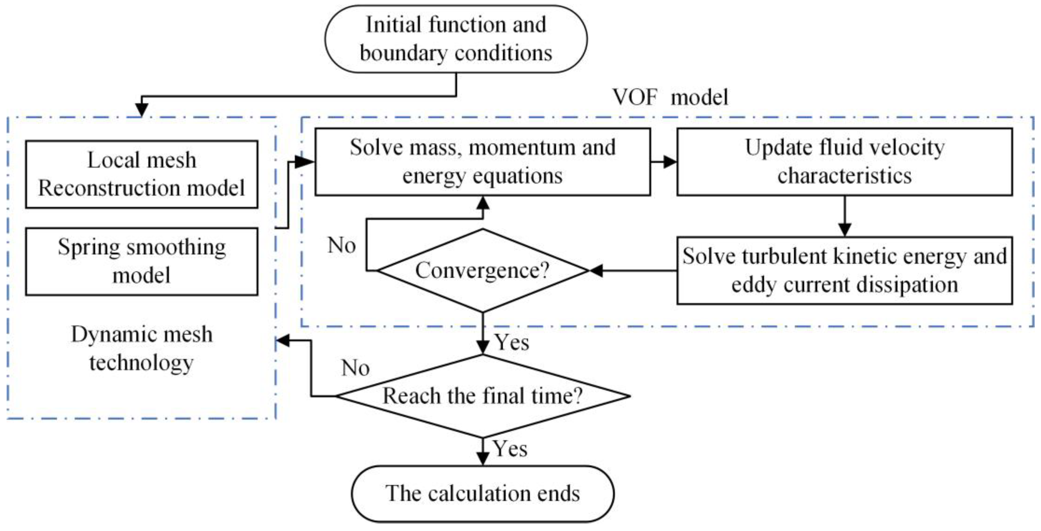
The oil agitation characteristics of the toothless gearbox are solved using the VOF model coupled with dynamic mesh technology, as illustrated in Figure 1. Initially, the initial conditions and boundary conditions are defined to ensure the accuracy of the physical setup in the simulation. Based on the initial mesh, the governing equations and turbulence dynamics equations are solved, and the VOF model is employed to track the two-phase interface [43,44]. Subsequently, the flow-field velocity characteristics are updated, and the turbulence kinetic energy and vortex dissipation are solved. Next, the convergence of the CFD model is assessed. If convergence is not achieved, the governing equations are re-solved; if convergence is achieved, the solution duration is then checked [45,46]. If the target duration is not reached, the mesh is updated using dynamic mesh technology to simulate the rotation process of the toothless gear, and the previous steps are repeated until the desired solution time is met [47,48]. This process enables precise simulation of oil agitation in the toothless gearbox. It allows for the analysis of fluid dynamics, providing a foundation for further optimization and performance enhancement.
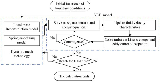
Figure 1.
Multistage transmission gear box solution strategy.
3. Numerical Model of the Gear Lubricating Oil Field
3.1. Geometric Model and Numerical Model
The gearless oil splash disc operates within a single-stage oil splash system, where it stirs the lubricating oil at the bottom of the housing and generates splashes to lubricate and cool the internal components of the system, as illustrated in Figure 2a. The lubrication system adopts a three-dimensional model, with boundary regions defined according to specific analysis requirements and boundary conditions to minimize unnecessary complexity. Since the shaft and bearing structures have minimal influence on the flow field, this study retains the actual shape of the splash disc to simulate its interaction with the lubricating oil, as well as the associated pressure distribution and airflow dynamics. The fluid domain model excludes the shaft and bearings. A three-dimensional fluid model is employed to calculate transient flow, with the basic parameters of the gearless oil splash disc provided in Figure 2b. The simplified oil tank model measures 270 × 190 × 15 mm, featuring grooves 20 mm wide on both sides, with lubricating oil filling the interior up to height h. The active splash disc on the left has a radius of 85 mm and a central hole with a radius of 12.5 mm. Two smaller holes, each with a radius of 3 mm, are symmetrically positioned. The fixed splash disc on the right features a convex elliptical shape with parallel sides. Its center includes a raised cylindrical platform, while a U-shaped groove is located below it. The simplified model preserves the essential geometric features of the core components and accurately reproduces the structure of the gearless oil tank.
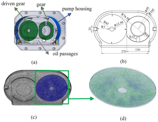
Figure 2.
Illustrates the model schematics. (a) Actual model. (b) Simplified model with dimensions. (c) Overall mesh. (d) Locally refined mesh.
This study utilizes ANSYS Fluent 19.0 for flow-field analysis during the geometry preprocessing phase. The software optimizes flow-field simulations by allowing for the separate extraction of external and internal fluid domains and enabling topology sharing. The geometry model of the oil stirrer disc is imported, and the fluid shell is extracted as the internal fluid domain of the stirrer disc housing. Within the working area of the stirrer disc, contact occurs at the agitation surface. However, boundary contact is not permitted in the fluid simulation module. Additionally, the fluid space in the agitation area is narrow, which may result in extremely small grid sizes in this region, creating significant discrepancies compared to the grid sizes in surrounding areas. These discrepancies can lead to grid deformation during iterative calculations and grid updates, potentially causing computational errors. Moreover, excessively small grid sizes significantly increase computation time. To address these issues, the center distance between the oil stirrer discs is increased by 1 mm, effectively reducing the grid size disparity and the total grid count within the working area.
After completing the geometry preprocessing, the fluid domain model is imported into the ANSYS meshing module. The external fluid domain is meshed using unstructured tetrahedral elements. This mesh type is particularly suitable for dynamic grid models, providing good mesh quality and high solution accuracy [49,50,51]. The results of the grid division are shown in Figure 2c. In theory, smaller mesh element sizes yield more accurate solutions. However, excessively fine meshes consume significant computational resources, greatly increasing solution time. Therefore, during meshing, local refinement is applied to regions with large variations in physical properties. This local refinement helps reduce solution time while maintaining an acceptable error range [52,53,54,55]. To ensure computational convergence and result accuracy, mesh refinement is applied to the stirrer disc and gap area, with mesh element sizes set to 1 mm. The mesh refinement results are shown in Figure 2d. The final mesh count is maintained at around 1 million, with approximately 200,000 nodes and a maximum skewness of less than 0.7.
3.2. Initial Conditions and Boundary Conditions
In the simulation of the gearless oil pan, the initial and boundary conditions are crucial for ensuring accuracy. The relevant parameters are listed in Table 1. At the beginning of the simulation, the oil pan is filled with lubricating oil. The initial temperature of the oil is set to ambient temperature (20 °C), and the initial velocity of the oil is zero, indicating that the system is stationary before startup. The density of the lubricating oil is 880 kg/m3, and its dynamic viscosity is 0.06 kg/(m·s). Both the oil pan and the lubricating oil are assumed to be at ambient temperature, reflecting the thermal state of the system before operation. The initial pressure within the oil pan is set to atmospheric pressure (101,325 Pa), simulating normal working conditions. A dynamic mesh model is employed during the simulation of component motion, with the oil pan defined as a rotating wall. The inner wall of the oil pan box is set as a no-slip wall, meaning that the velocity of the lubricating oil at the wall is zero.

Table 1.
Basic parameters of the toothless agitator oil tank.
The following steps are involved in the simulation: Import the finite element mesh model into fluid simulation software. Use a user-defined function (UDF) program to set the dynamic behavior of the gear while applying restrictions on the mesh update parameters. Employ a pressure-based solver for the simulation, setting the time step to 2 × 10⁻⁵ s and the residual convergence criterion to 1 × 10⁻⁵ [56,57,58,59]. After the simulation reaches convergence, analyze the results. For multiphase flow analysis, select the volume-of-fluid (VOF) model combined with the RNG k-ε turbulence model [60,61,62,63,64]. Near the wall, apply the standard wall function. In the solver settings, use the standard SIMPLE algorithm for pressure-velocity coupling, the least squares method for gradient discretization, the PRESTO algorithm for pressure treatment, and the second-order upwind scheme for turbulence kinetic energy [65,66,67].
3.3. Grid Independence Verification
The high-quality grid effectively enhances the accuracy of numerical computations, thereby ensuring the precision of the solution [68,69,70]. To further enhance the reliability of the simulation, this study optimized several key parameters in the grid discretization process. Specifically, the spring constant factor was set to 0.1, the convergence tolerance to 0.0001, and the maximum number of iterations to 1000. During local grid re-discretization, the maximum cell skewness was set to 0.82, the maximum face skewness to 0.7, and the grid size reconstruction interval to 5. These settings ensured the quality of the grid while mitigating potential errors in the computation. Moreover, appropriate grid scaling is crucial for achieving both efficient and accurate numerical results. Coarse grids can result in significant solution errors or even divergence, while excessively fine grids increase computational resource requirements and extend solution time [71,72]. To balance computational accuracy and efficiency, this study conducted simulations with four different grid scales for the toothless oil agitation tank numerical model: N1 = 328,751, N2 = 491,462, N3 = 726,025, and N4 = 1,079,654. Since this study primarily focuses on the oil agitation process, the oil velocity distribution along the x-axis in the agitation region was obtained, as shown in Figure 3. The results indicated that, with larger grid scales (N1 and N2), the solution accuracy was lower. As the grid was refined, solution accuracy steadily increased. When the grid scale reached N3, the relative error compared to N4 was less than 3%. In conclusion, the N3 grid scale offers a balance between solution accuracy and computational resource efficiency.
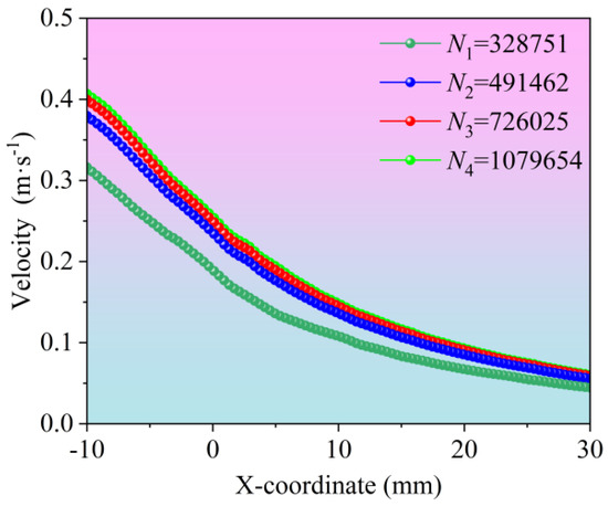
Figure 3.
Grid independence verification.
4. Numerical Simulation of Gear Lubricating Oil Field
4.1. Lubricating Oil Distribution in High-Speed Gearbox
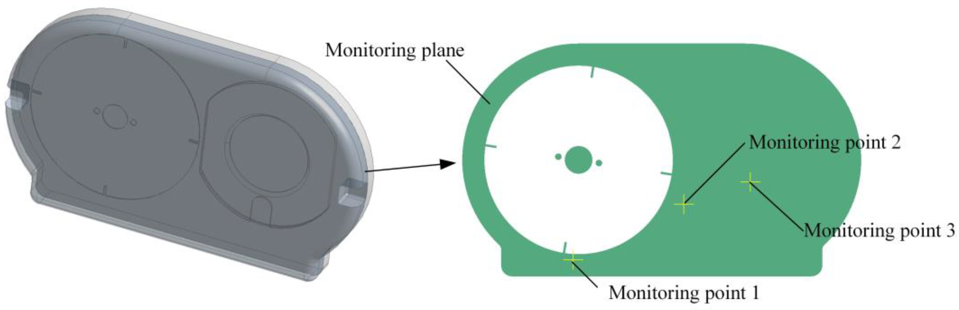
In order to monitor the changes of various parameters inside the oil sump over time, three different monitoring points were set up based on the monitoring surface shown in Figure 4, to grasp the dynamic changes of the flow-field parameters inside the oil sump. Among them, monitoring point 1 is located directly below the oil pan, used to capture the flow-field changes in the area beneath the oil pan. Monitoring point 2 is set at the tangent position of the oil pan, monitoring the parameter changes of the fluid as it leaves the oil pan at that point. Monitoring point 3 is located in the central area on the right side of the oil sump, observing the dynamic flow-field parameters in the central area on the right side of the oil sump. Through the reasonable layout of these three monitoring points, a comprehensive observation of the changes in the flow-field parameters inside the oil sump is achieved, allowing for an in-depth exploration of the evolution patterns of the flow field in the oil sump.
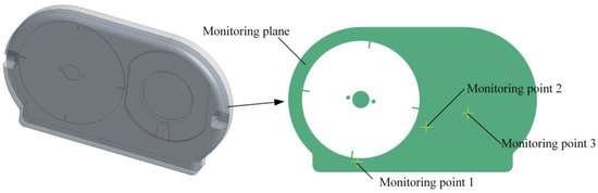
Figure 4.
Distribution of monitoring points.
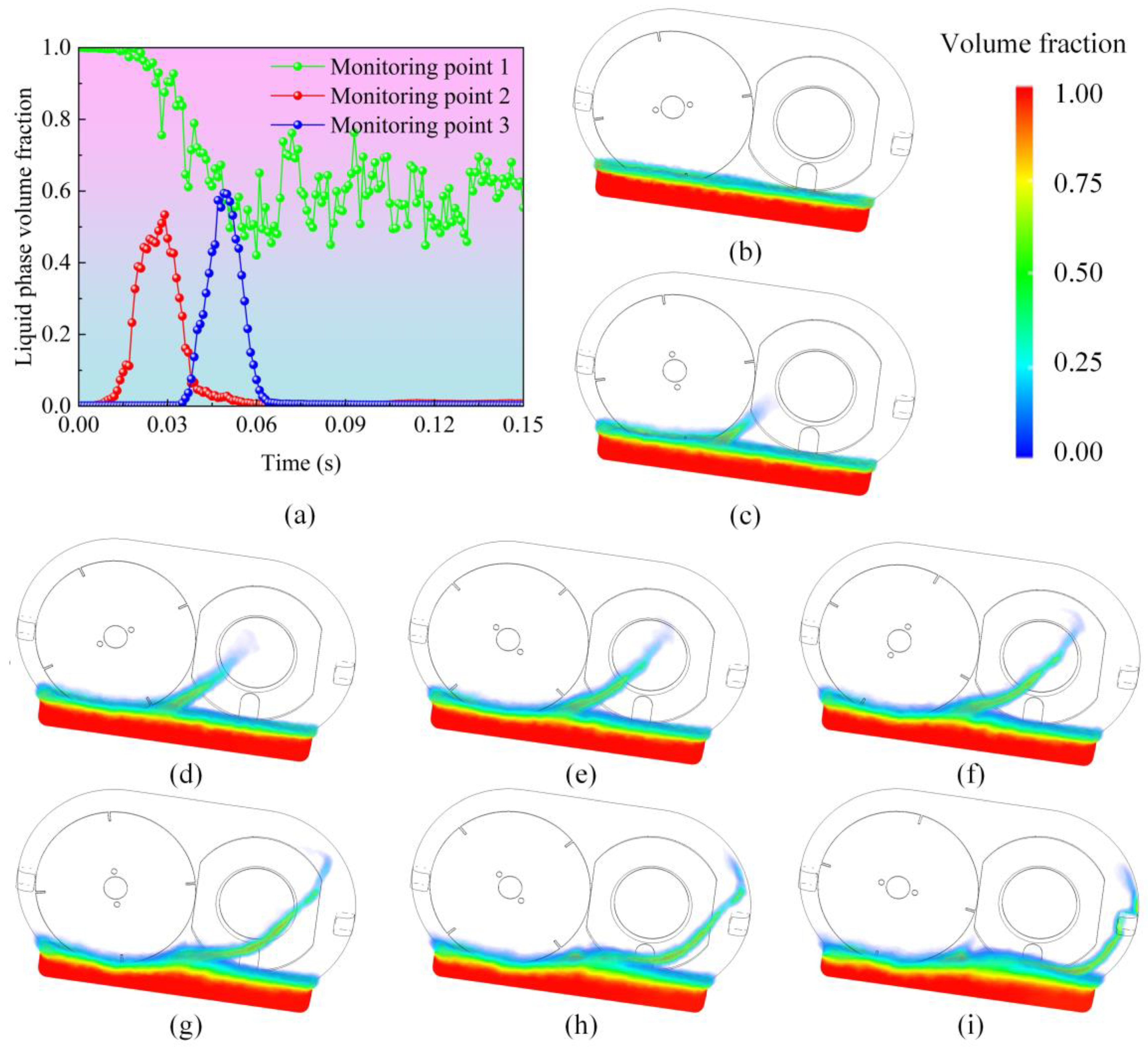
To explore the variation law of the liquid volume fraction, curves of the liquid phase volume fraction at each monitoring point over time were plotted, as shown in Figure 5a. By analyzing the curves of the liquid phase volume fraction over time at different monitoring points, the movement patterns of the oil liquid inside the mixing tank were revealed. At monitoring point 1, the liquid phase volume fraction changed a little from 0 to 0.03 s. As the stirring continued, the liquid phase volume fraction gradually decreased and oscillations appeared at 0.06 s. This is because, in the initial stage, the amount of oil liquid stirred up by the mixing disk was small, having a limited effect on the oil liquid below; as stirring continued, more oil liquid was stirred up, causing the liquid level to drop and resulting in significant oscillations, leading to fluctuations in the volume fraction at monitoring point 1 around 0.06 s. At monitoring point 2, the liquid phase volume fraction rapidly increased from 0 to 0.015 s but then decayed to zero after 0.015 s. This was due to the oil liquid being stirred up by the mixing disk and leaving the position of monitoring point 2. Subsequently, the oil liquid migrated to the central area on the right where monitoring point 3 is located, causing the liquid phase volume fraction at monitoring point 3 to rise to 0.6 at 0.05 s, followed by a rapid decay. In summary, during the initial stage, the liquid phase volume fractions at all monitoring points exhibited significant volatility, which then gradually stabilized. These results are significant for understanding the evolution of the flow field and liquid phase distribution in the lubrication system of a toothless mixing disk, and they help optimize the design and operation of the lubrication system.
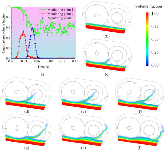
Figure 5.
Evolution process of gearbox lubricating oil. (a) Time-varying curves of liquid phase volume parameters at different monitoring points. (b) 0 s. (c) 0.015 s. (d) 0.03 s. (e) 0.045 s. (f) 0.06 s. (g) 0.09 s. (h) 0.12 s. (i) 0.15 s.
To obtain a clear view of the oil distribution, a distribution map of the oil volume fraction was obtained, as shown in Figure 5b–i. In the initial state, only the red part at the bottom of the oil sump is the fluid domain of the oil sump. This figure reveals the process of lubricating oil splashing into the working area of the oil sump. The oil volume fraction reflects the ability of the lubricating oil to penetrate the airflow and enter the working area for lubrication. This paper observes the liquid phase distribution inside the oil sump at different moments: 0 s, 0.015 s, 0.03 s, 0.045 s, 0.06 s, 0.09 s, 0.12 s, and 0.15 s. From the figure, it can be observed that the flow field generated by the high-speed rotating oil sump significantly affects the movement and distribution of the oil. From 0 s to 0.015 s, the oil is lifted by the oil sump due to the adhesion effect of the wall. Subsequently, from 0.015 s to 0.9 s, the oil in the working area of the oil sump aligns with the direction of the flow field, forming a temporary oil accumulation area at the top of the oil sump, with some oil diffusing above the oil sump and being carried into the working area after colliding with the stirring disk. At this time, the amount of oil taken away by the stirring disk on the right side is relatively small, as shown in Figure 5d–g. As time progresses from 0.12 s to 0.15 s, most of the lubricating oil adheres around the stirring disk of the oil sump. The stirring oil pan moves until it approaches the working area, where it detaches from the attachment area due to the interference of another oil flow, as shown in Figure 5h,i. The area of oil accumulation on the right side of the stirring pan gradually expands, reaching its maximum value at 0.15 s. The lubricating oil attached to the right side of the stirring pan shows a tendency to detach from the stirring oil pan, and the color of the oil volume fraction on the oil pan deepens, indicating that the amount of oil carried away by the stirring pan has increased. The interaction between the oil and the stirring surface has stabilized, and eventually, the oil splashes onto the wall of the stirring oil pan.
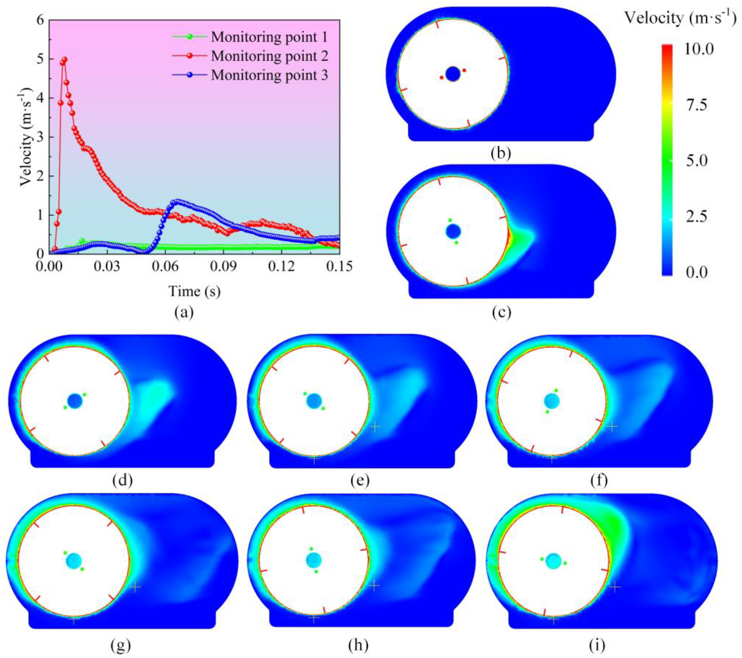
The analysis of lubrication speed plays an important role in enhancing the load capacity of gears, reducing the risk of failure, and extending their service life. By studying the lubrication speed of gears, we can predict the flow and distribution of lubricating oil in the gear area, which is crucial for improving the design of lubrication systems and enhancing lubrication efficiency. Figure 6 shows the variation in lubricating oil speed over time. Figure 6a presents the time-varying curves of speed at different monitoring points. At monitoring point 1, the flow field is disturbed by the oil slinger, resulting in some fluctuations; however, due to its distance from the gear edge and the lower liquid level, the degree of disturbance is relatively low. At monitoring point 2, there is a sharp increase in speed at 0.01 s, reaching a peak value of 5 m/s. This is because the oil slinger throws off the adhered oil at a higher speed. Subsequently, the flow-field speed at monitoring point 2 shows a certain decline. Since monitoring point 3 is located at the right center, when the thrown-off oil reaches this area, energy has already dissipated. Therefore, at 0.07 s, the flow-field speed at monitoring point 3 experiences a slight increase followed by a slow decline. The analysis of the time-varying curves of flow-field speed at different monitoring points indicates that in the initial stage, the oil slinger throws the oil out at a high initial speed, and then dissipation occurs in the right space, leading to a decrease in oil speed.

Figure 6.
Cloud map of lubrication oil velocity in the gearbox. (a) Time-varying velocity curves at different monitoring points. (b) 0 s. (c) 0.015 s. (d) 0.03 s. (e) 0.045 s. (f) 0.06 s. (g) 0.09 s. (h) 0.12 s. (i) 0.15 s.
To analyze the variation of oil velocity in the flow field, observations were made at different times: 0 s, 0.015 s, 0.03 s, 0.045 s, 0.06 s, 0.09 s, 0.12 s, and 0.15 s, to examine the velocity distribution in the oil mixing tank, as shown in Figure 6b–i. In Figure 6b–e, the color changes at the edges of the gears are quite pronounced, indicating that there are significant velocity gradients in these areas. This is caused by the high-speed rotation of the oil mixing disk and the interaction between the lubricating oil. As the mixing disk stirs, the momentum of the lubricating oil continuously increases, leading to higher velocities. Some lubricating oil, influenced by centrifugal force and gravity, may detach from the mixing disk and continue to splash under the action of inertial forces, as shown in Figure 6f. In the gearbox, the lubricating oil on the mixing disk accelerates due to compression, and then this compressed lubricating oil flows to the bottom of the tank and quickly integrates into the lubrication cycle of the entire flow field. This cycle helps the lubricating oil to distribute evenly throughout the gearbox. In the cloud diagrams of Figure 6g–i, the distribution of lubricating oil near the gears is more uniform, indicating that the lubrication system can effectively cover the gear surfaces at these time points, reducing friction and wear. Overall, these cloud diagrams provide an intuitive view of the flow of lubricating oil in the gearbox, aiding in the analysis of lubrication efficiency and identifying areas that may need improvement. With this information, adjustments can be made to the lubrication system to enhance the performance and reliability of the gearbox.
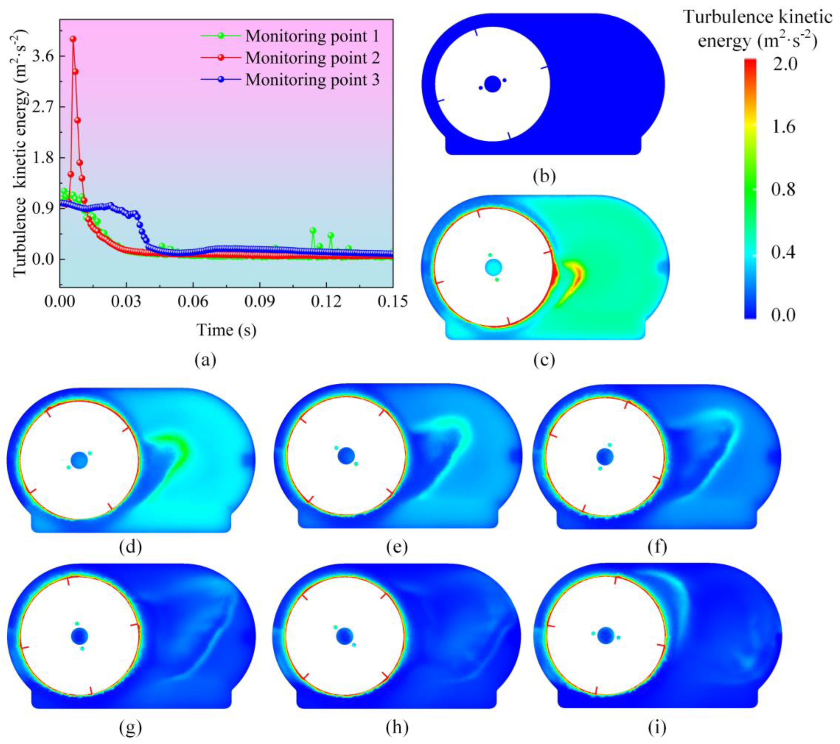
Turbulent kinetic energy analysis helps to understand the variation patterns of the complex two-phase oil–gas flow inside the gearbox, which is crucial for ensuring the normal and efficient operation of the gearbox. Figure 7a shows the evolution curves of turbulent kinetic energy at different monitoring points. It can be observed that the amplitude of turbulent kinetic energy at monitoring point 2 can reach 4.0 m2/s2. The changes in turbulent kinetic energy at the other two monitoring points are not significant. Figure 7b–i describes the turbulent kinetic energy evolution contour map of the gear oil stirring plate. It can be seen that the distribution of turbulent kinetic energy around the gearbox is uneven, especially in the edge areas of the gears and the gearbox body. In the initial stage (Figure 7c), turbulent kinetic energy is mainly concentrated in the central area of the gear. The lubricating oil is subjected to shear from the stirring plate, which is the main source of turbulent energy generation. Therefore, a higher turbulent kinetic energy is displayed in the area near monitoring point 2. Over time, the turbulent energy propagates outward from the left gear area, manifested as a high turbulent kinetic energy region expanding outward from the center of the gear, as shown in Figure 7d–f. This is caused by the rotational motion of the stirring plate. After 0.06 s, a circulation flow pattern of turbulent kinetic energy forms around the gear. This circulation helps to evenly distribute turbulence throughout the gearbox. However, in areas far from the gear meshing zone, the turbulent energy gradually dissipates due to friction and energy loss. This characteristic is reflected in the transition of the cloud map colors from green to blue. In the cloud map at 0.12 s, the distribution of turbulent kinetic energy is more uniform. This indicates that the lubrication system can effectively cover the gear surface at this time point, but it also increases turbulence. Turbulence can affect the stability of the lubrication film. In regions with high turbulent energy, the lubrication film is thinner, which increases the risk of wear on the gear surface. These cloud maps can help identify areas with higher turbulence intensity, which aids in taking measures in gearbox design, such as optimizing gear shapes, adjusting gear spacing, or changing lubrication oil properties, to reduce turbulence and improve efficiency.

Figure 7.
Turbulent kinetic energy cloud map of the gearbox lubricating oil. (a) Time-varying curves of turbulent kinetic energy at different monitoring points inside the oil mixing tank. (b) 0 s. (c) 0.015 s. (d) 0.03 s. (e) 0.045 s. (f) 0.06 s. (g) 0.09 s. (h) 0.12 s. (i) 0.15 s.
4.2. Different Oil Distribution at Various Rotational Speeds
In the gear lubrication process, the rotational speed of the gears and the height of the oil have a significant impact on the lubrication effect. Figure 8 illustrates the flow of lubricating oil inside the gearbox at 0.15 s under different conditions: rotational speeds (3200, 3600, 4000 rpm) and oil heights (10, 15, 20 mm). At higher rotational speeds, the flow of lubricating oil tends to appear more red and yellow, indicating higher speeds. For example, when the oil height is 10 mm, at a rotational speed of 3200 rpm, the flow of lubricating oil is relatively steady with minimal turbulence. When the speed increases to 3600 rpm, the acceleration of oil flow becomes more pronounced, and turbulence becomes more noticeable, especially on the right side of the gearbox. At the higher speed of 4000 rpm, the free surface of the liquid phase exhibits intense fluctuations, and turbulence reaches its peak, leading to more aggressive splashing and circulation of the lubricating oil. Therefore, higher speeds cause more noticeable vortices at the bottom of the gearbox, resulting in the breakdown of the oil film, which affects the distribution of lubricating oil and the lubrication effect on the gears.
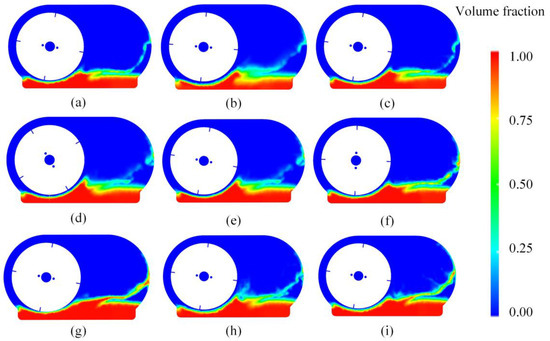
Figure 8.
Distribution of liquid phase volume fraction under different operating conditions. (a) n = 3200 r/min, h = 10 mm. (b) n = 3600 r/min, h = 10 mm. (c) n = 4000 r/min, h = 10 mm. (d) n = 3200 r/min, h = 15 mm. (e) n = 3600 r/min, h = 15 mm. (f) n = 4000 r/min, h = 15 mm. (g) n = 3200 r/min, h = 20 mm. (h) n = 3600 r/min, h = 20 mm. (i) n = 4000 r/min, h = 20 mm.
The oil height significantly influences the flow characteristics of the lubricating oil within the gearbox. An appropriate oil height ensures even distribution of the oil, covering the gear surfaces and providing effective lubrication. As shown in Figure 8, at a rotational speed of 3200 rpm, a lower oil height (10 mm) limits oil splashing, whereas at an oil height of 20 mm, a more stable oil film forms. At an oil height of 15 mm, the increased height allows the lubricating oil to form an unstable film on the right side of the gearbox, which enhances lubrication performance. When the oil height reaches 20 mm, a stable oil film is also formed at the higher speed of 4000 rpm. Different oil heights lead to variations in the circulation path of the lubricating oil within the gearbox. As the oil splashes and circulates more noticeably, the distribution of the lubricating oil across the gear surfaces becomes more uniform. While increasing the oil immersion depth is crucial for improving lubrication between gears and bearings, it may also introduce some negative effects, such as increased friction, elevated casing temperatures, and higher energy losses during the agitation of the oil. These factors can lead to a reduction in transmission efficiency. In contrast, reducing the oil immersion depth may decrease oil losses and mitigate temperature rise, but this could result in insufficient lubrication for the gears and bearings, thereby reducing the lifespan of the gearbox. Therefore, when determining the optimal oil immersion depth, a balance must be struck between ensuring effective lubrication and minimizing immersion depth to maximize transmission efficiency and minimize operational costs. This requires careful design of the oil immersion depth to optimize lubrication, while controlling friction and temperature rise to ensure the gearbox’s long-term stable operation.
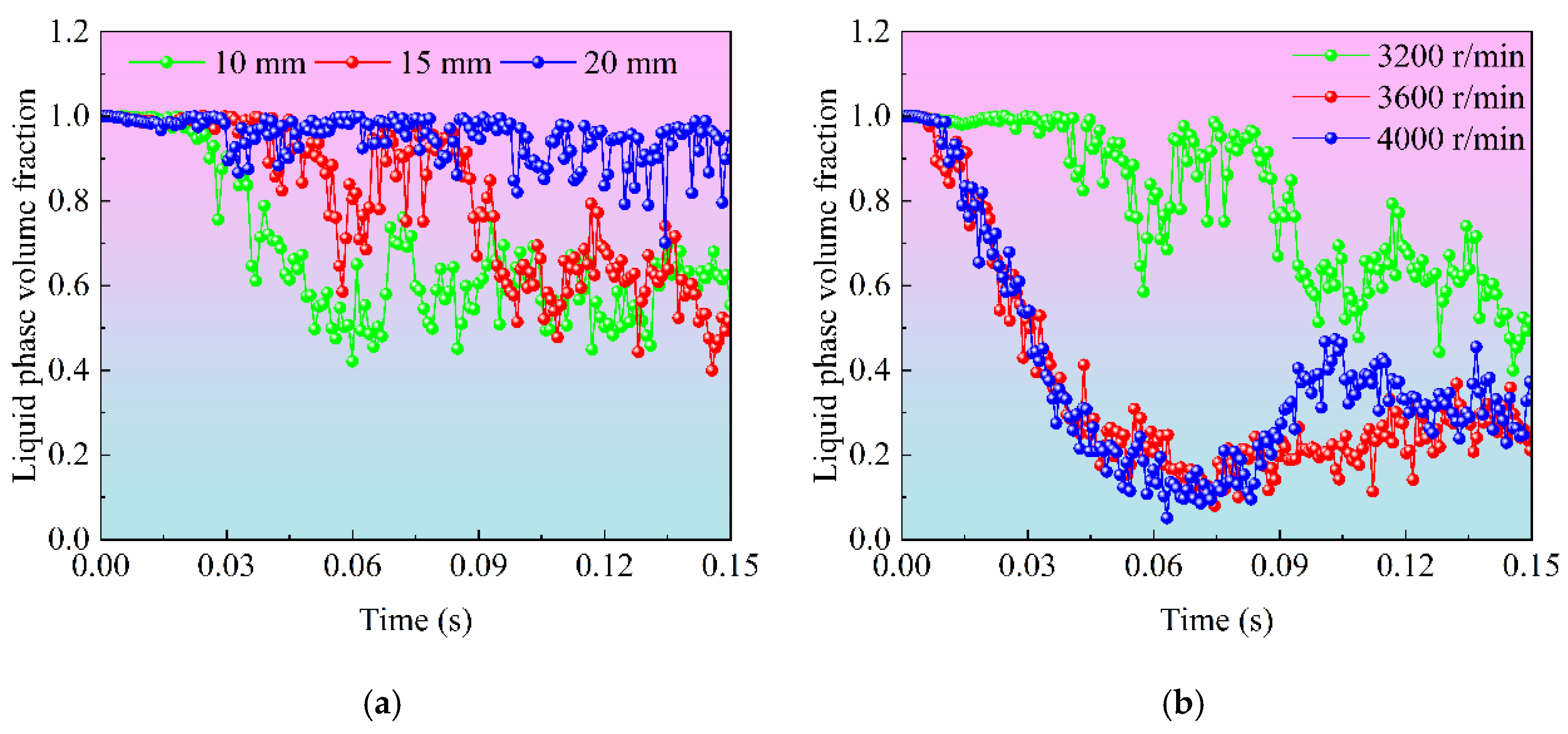
Figure 9 illustrates the evolution of the liquid phase volume fraction at monitoring point 1 within the gearbox under various conditions, including different rotational speeds (3200, 3600, 4000 rpm) and oil heights (10, 15, 20 mm). In Figure 9a, the volume fraction at monitoring point 1 exhibits significant oscillations at different oil heights. When the oil height is 20 mm, the variation in liquid phase volume fraction is relatively small. However, at lower oil heights (10 mm and 15 mm), the volume fraction shows substantial oscillations, with the fraction decreasing to as low as 0.4. Over time, the volume fraction fluctuates stably between 0.4 and 0.8. This phenomenon suggests that a higher oil height results in greater fluid agitation, with higher peak and stable values of the liquid phase volume fraction. In Figure 9b, as the rotational speed increases, the liquid phase volume fraction at monitoring point 1 decreases continuously. This indicates that with higher rotational speeds, the lubricating oil is more agitated, and its splash height increases, leading to a reduction in the liquid phase at this location. The increase in the stirrer speed accelerates the oil splashing. However, once the stirrer speed reaches a certain level, further increases do not significantly enhance the stirring effect. The higher the stirrer speed, the greater the peak and stable values of the liquid phase volume fraction. Overall, by adjusting parameters such as oil height and stirrer speed, the liquid phase volume fraction can be optimized to achieve the best lubrication performance.
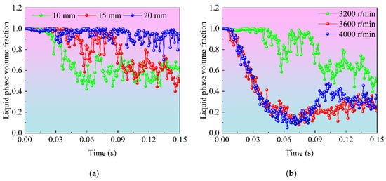
Figure 9.
Liquid phase volume fraction under different operating conditions. (a) Liquid phase volume fraction at different oil heights. (b) Liquid phase volume fraction at different stirrer speeds.
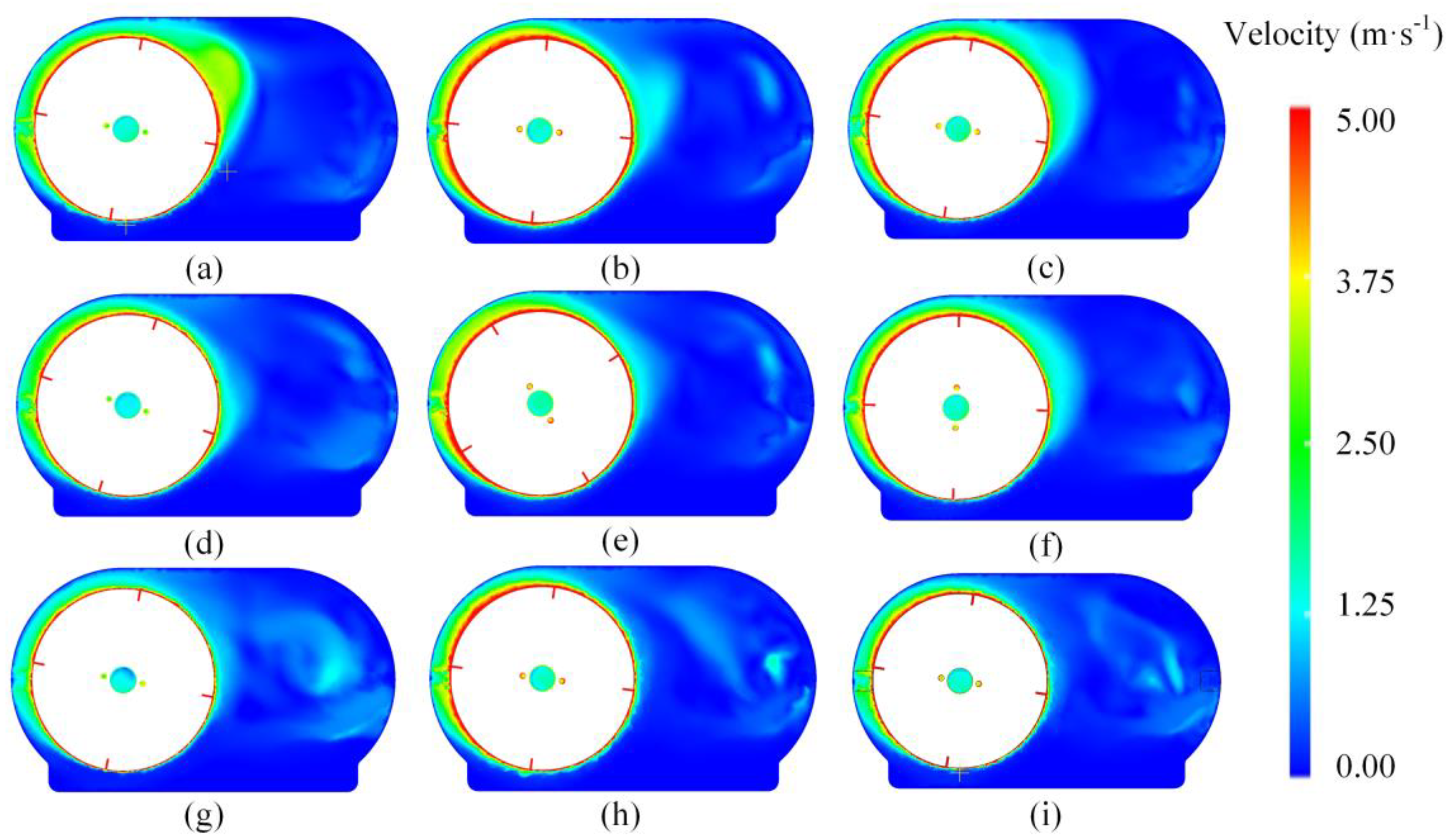
Figure 10 shows the velocity distribution cloud map of the lubricating oil inside the gearbox at 0.15 s under different rotational speeds (3200, 3600, 4000 r/min) and different oil heights (10, 15, 20 mm). From the figure, it can be observed that at a lower oil height of 10 mm, the velocity distribution near the left-side gear is uniform. As the oil height increases, the liquid phase velocity in local regions gradually decreases. Under the same oil height, changes in rotational speed have a negligible effect on the velocity distribution. In some regions on the right side, vortex evolution of the liquid phase velocity can be seen, as shown in Figure 10g–i. This suggests that under the same oil height, increasing the stirrer speed has little impact on the overall oil velocity distribution in the flow field.
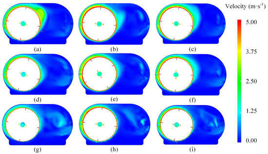
Figure 10.
Velocity distribution of the lubricating oil under different operating conditions. (a) n = 3200 r/min, h = 10 mm. (b) n = 3600 r/min, h = 10 mm. (c) n = 4000 r/min, h = 10 mm. (d) n = 3200 r/min, h = 15 mm. (e) n = 3600 r/min, h = 15 mm. (f) n = 4000 r/min, h = 15 mm. (g) n = 3200 r/min, h = 20 mm. (h) n = 3600 r/min, h = 20 mm. (i) n = 4000 r/min, h = 20 mm.
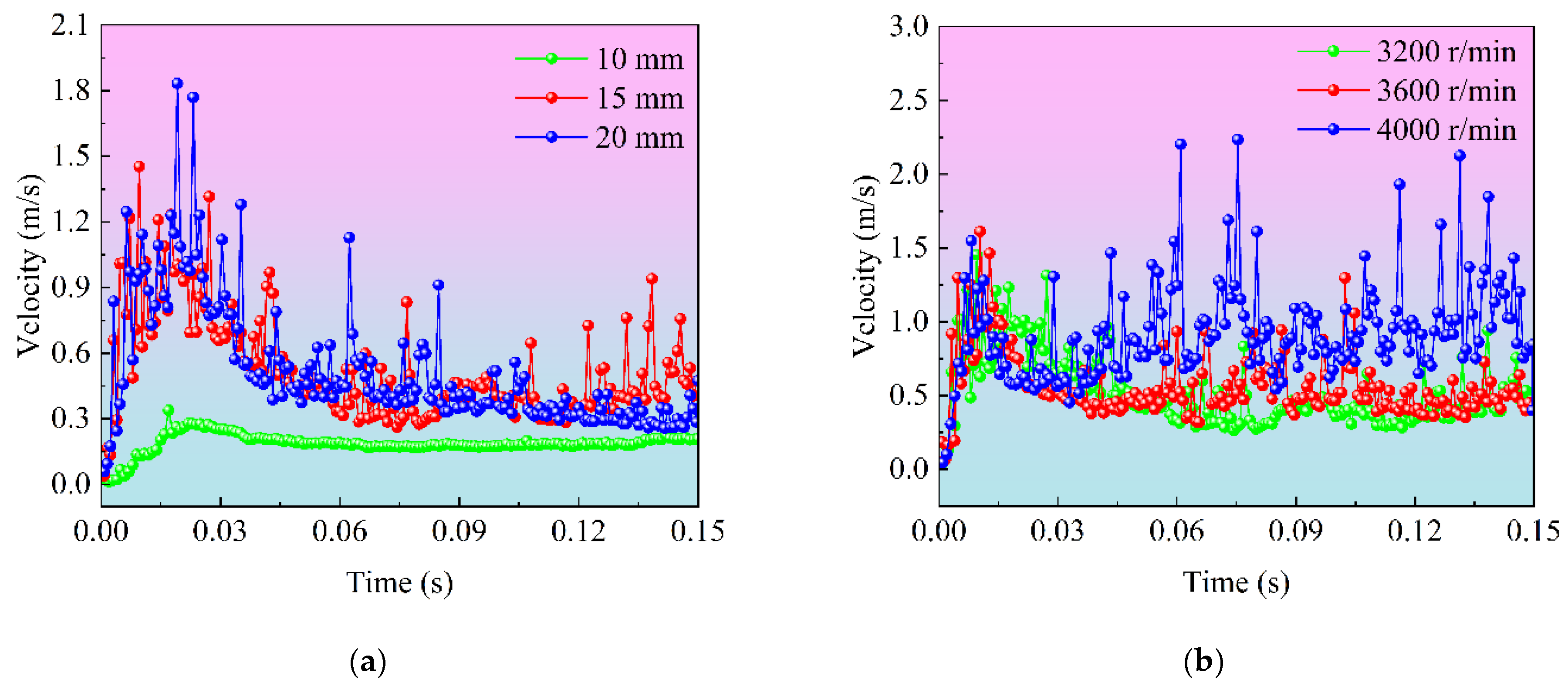
To analyze the evolution of the oil velocity, the velocity trends at monitoring point 1 in the gearbox under different rotational speeds (3200, 3600, 4000 r/min) and oil heights (10, 15, 20 mm) were obtained, as shown in Figure 11. From Figure 11a, it can be observed that when the oil height is 10 mm, the velocity change at monitoring point 1 is small. As the oil height increases to 15 mm and 20 mm, the velocity at monitoring point 1 rapidly increases and then decreases, accompanied by more nonlinear pulse amplitudes. This indicates that the increase in oil height enhances the turbulence velocity in the flow field, increases the disorder, and promotes the agitation of the oil. In Figure 11b, under the same oil height, as the speed increases, the disturbances at monitoring point 1 continuously increase, and its velocity structure exhibits stronger nonlinear pulse characteristics. This phenomenon suggests that under conditions of higher oil height and higher speed, the stirrer induces larger disturbances at monitoring point 1, causing the flow-field velocity to exhibit highly nonlinear characteristics, thereby improving the efficiency of the oil mixing process.

Figure 11.
Lubricating oil velocity under different operating conditions. (a) Oil velocity at different oil heights. (b) Oil velocity at different stirrer speeds.
When the gearbox is running, the rotation of the gears causes the lubricant at the bottom of the box to oscillate. The lubricant swirls along the curved walls of the housing, disrupting the laminar flow of the fluid, and leading to turbulence. The energy of the turbulence is referred to as turbulence intensity, which is proportional to the turbulent viscosity. Turbulent viscosity has a viscous effect on the rotation of the gears, causing energy loss in the oil agitation. Vortex viscosity is used to quantify the viscous effects of turbulence, helping to more accurately simulate and predict the complex flow behavior inside the gearbox. Figure 12 illustrates the vortex viscosity variation at 0.15 s under different operating conditions inside the gearbox. From the figure, it can be seen that, under the same gear speed, the vortex viscosity is higher at the center of the gear bottom, shown as red and yellow regions. The fluid in these regions is affected by the agitation of the oil agitator, producing higher turbulence intensity. As the speed increases from 3200 r/min to 4000 r/min, the agitation of the oil increases, thereby enhancing the turbulence. However, vortex viscosity does not always increase. For example, at 3200 r/min, the different oil heights have little effect on the flow and agitation inside the gearbox. When the speed reaches 3600 r/min, the vortex viscosity at the center-bottom area reaches its maximum, showing as an expansion or deepening of the red area. But at 4000 r/min, vortex viscosity decreases at the center-bottom region. Under the same speed conditions, higher oil height increases the agitation of the lubricant, allowing it to flow over a larger area, but the variation in vortex viscosity is minimal. This is because speed and immersion depth work together to affect how the lubricating oil flows. The rotating speed of the gear decides how hard and in which direction the lubricating oil is stirred. The immersion depth influences the initial distribution of the lubricating oil and the space where it can flow. When the rotating speed is high and the immersion depth is large, it will make the lubricating oil in the gearbox create stronger turbulence. We can see this interaction from the changes in eddy viscosity. Under the condition of the same rotating speed, a higher oil level will make the lubricating oil be stirred more vigorously. It allows the lubricating oil to flow over a larger range and generate more turbulence. As the rotating speed increases, the force with which the gear stirs the lubricating oil becomes greater, and the turbulence also becomes stronger. In-depth research and analysis of vortex viscosity can provide important scientific guidance for the design, maintenance, and optimization of gearboxes.
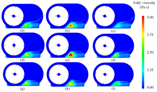
Figure 12.
Vortex distribution under different operating conditions. (a) n = 3200 r/min, h = 10 mm. (b) n = 3600 r/min, h = 10 mm. (c) n = 4000 r/min, h = 10 mm. (d) n = 3200 r/min, h = 15 mm. (e) n = 3600 r/min, h = 15 mm. (f) n = 4000 r/min, h = 15 mm. (g) n = 3200 r/min, h = 20 mm. (h) n = 3600 r/min, h = 20 mm. (i) n = 4000 r/min, h = 20 mm.
Figure 13 shows the distribution of turbulent kinetic energy (TKE) at 0.15 s under different operating conditions inside the gearbox. These contour plots help to understand the variation in turbulent kinetic energy under different speed and oil height conditions. The color change in the figure represents the magnitude of turbulent kinetic energy, where red and yellow regions indicate higher TKE and blue regions represent lower TKE. At the same speed of 3200 r/min, as the oil height increases, the turbulent kinetic energy in the right-side region of the gearbox increases. This indicates that the turbulence intensity strengthens with the increase in oil height. Additionally, when the speed is 3600 r/min and 4000 r/min, the turbulent kinetic energy in the right-side region of the gearbox is also higher when the oil height is 20 mm. This phenomenon is not as prominent at oil heights of 10 mm and 15 mm. The process is caused by the oil splashing into the gearbox to prevent impact, with the oil mixing with air during the splash. After the oil–air mixture splashes to the right-side housing, the oil flows back into the oil pool along the baffle. Based on the analysis of turbulent kinetic energy, control strategies can be developed to reduce unnecessary turbulence, such as optimizing gearbox design, adjusting lubricant properties, or using additives to improve the flow characteristics of the lubricant.
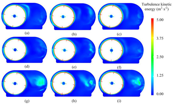
Figure 13.
Distribution of turbulent kinetic energy under different operating conditions. (a) n = 3200 r/min, h = 10 mm. (b) n = 3600 r/min, h = 10 mm. (c) n = 4000 r/min, h = 10 mm. (d) n = 3200 r/min, h = 15 mm. (e) n = 3600 r/min, h = 15 mm. (f) n = 4000 r/min, h = 15 mm. (g) n = 3200 r/min, h = 20 mm. (h) n = 3600 r/min, h = 20 mm. (i) n = 4000 r/min, h = 20 mm.
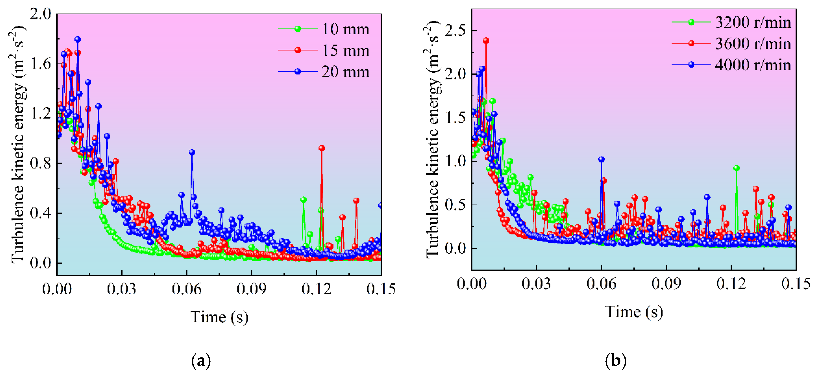
Figure 14 shows the evolution trend of turbulent kinetic energy at monitoring point 1 under different operating conditions. In Figure 14a, the variation in turbulent kinetic energy at different oil heights is presented. From the figure, it can be observed that at the initial moment, the turbulent kinetic energy at all oil heights increases rapidly, reaching a peak value. The turbulent kinetic energy at 20 mm oil height reaches its highest value, close to 1.8 m2/s2. In the middle phase (0.03–0.06 s), as the agitation process evolves, the turbulent kinetic energy decreases continuously at different oil heights. At 20 mm oil height, it drops to 0.4 m2/s2, while at 10 mm and 15 mm oil heights, it decreases to 0.2 m2/s2. Due to the nonlinear turbulent process of the agitation flow field, there are instances of abrupt changes in amplitude. Figure 14b shows the trend of turbulent kinetic energy at different agitator speeds. The evolution trend is consistent with the variation in turbulent kinetic energy at different oil heights. As the agitation process evolves, the turbulent kinetic energy at 4000 r/min stabilizes at 0.2 m2/s2, while at 3200 r/min and 3600 r/min, it stabilizes at 0.3 m2/s2. The higher the oil height, the higher the peak of turbulent kinetic energy, indicating that a higher oil height produces stronger turbulence. Similarly, the higher the agitator speed, the higher the stable value of turbulent kinetic energy, generating stronger and more stable turbulence. By optimizing oil height and agitator speed, lubrication effectiveness can be improved, wear reduced, and equipment lifespan extended.

Figure 14.
Variation in turbulent kinetic energy under different operating conditions. (a) Turbulent kinetic energy at different oil heights. (b) Turbulent kinetic energy at different agitator speeds.
5. Conclusions
The transmission system is a critical component in the power transmission process, and the lubrication condition of the gearbox, as a key technical parameter, directly influences the reliability, power performance, and efficiency of mechanical transmission devices. By analyzing the oil agitation lubrication flow behavior within the gearbox and examining the dynamic evolution of the gear lubrication process under varying speeds and oil levels, theoretical insights can be provided for optimization strategies aimed at improving transmission efficiency. The main findings and conclusions of this study are summarized as follows:
1. A dynamic model of the lubrication process in a high-speed gearbox was developed using the volume of fluid (VOF) model and the RNG k-ε turbulence model, in conjunction with dynamic mesh technology that incorporates spring stiffness and grid reconstruction. The study analyzed factors such as volume fraction, turbulent kinetic energy, velocity, and vortex viscosity to investigate the flow behavior and oil distribution patterns in the gear lubrication process. Additionally, the influence of gear agitator speed and oil height on the lubrication process was assessed.
2. The speed of the agitator plays a pivotal role in the lubrication efficiency of the gears. At high agitator speeds, the lubricant, influenced by the combined effects of centrifugal force and gravity, detaches from the gear surface and splashes outward due to inertia. In the lower region of the gearbox, the lubricant is compressed and accelerated before flowing toward the gearbox bottom, rapidly integrating into the lubrication circulation system throughout the gearbox. This circulation process facilitates a more uniform lubricant distribution, thereby optimizing the lubrication performance.
3. Increasing the oil level is vital for improving the lubrication efficiency of the gears and bearings. When the speed is set to 3200 r/min and the oil height is 20 mm, a stable oil film is formed within the gearbox. Variations in the oil level alter the circulation path of the lubricant within the gearbox. Adjusting the oil level enhances the splashing and circulation of the lubricant, ensuring more even coverage of the gear surface and thereby improving lubrication effectiveness.
4. As the gear speed increases, the intensity of lubricant agitation increases, amplifying the turbulence effect. The difference in oil level significantly affects the flow pattern of the lubricant within the gearbox, influencing the distribution of turbulent kinetic energy. Higher agitator speeds lead to elevated stable values of turbulent kinetic energy, thereby enhancing the lubrication effect. By optimizing both the oil level and speed, lubrication performance can be improved, reducing wear on gears and bearings and effectively extending the equipment’s service life.
Author Contributions
Conceptualization, Y.H.; methodology, Y.H.; software, Y.H.; validation, G.Z.; formal analysis, Y.H.; investigation, Y.H.; resources, Y.H.; data curation, G.Z.; writing—original draft preparation, Y.H.; writing—review and editing, G.Z.; visualization, G.Z.; supervision, M.G.; project administration, G.Z.; funding acquisition, M.G. All authors have read and agreed to the published version of the manuscript.
Funding
This research received no external funding.
Data Availability Statement
The original contributions presented in this study are included in the article. Further inquiries can be directed to the corresponding author.
Conflicts of Interest
The authors declare no conflicts of interest.
References
- Hu, S.; Gong, W.; Gui, P. Numerical study on the churning power loss of spiral bevel gears at splash lubrication system. Lubr. Sci. 2024, 36, 259–276. [Google Scholar] [CrossRef]
- Jia, F.; Wang, B.; Fu, Y. A Novel Prediction Model for Churning Power Loss of Spur Gear. Lubr. Sci. 2024, 36, 645–655. [Google Scholar] [CrossRef]
- Li, Q.H.; Xu, P.; Li, L.; Xu, W.X.; Tan, D.P. Investigation on the Lubrication Heat Transfer Mechanism of the Multilevel Gearbox by the Lattice Boltzmann Method. Processes 2024, 12, 381. [Google Scholar] [CrossRef]
- Zheng, G.A.; Xu, P.; Li, L. Investigate on the Fluid Dynamics and Heat Transfer Behavior in an Automobile Gearbox based on the LBM-LES Model. Lubricants 2025, in press. [Google Scholar]
- Ji, R.Q.; Shen, Q.T.; Zhang, L.; Zeng, X.; Qi, H. Novel photocatalysis-assisted mechanical polishing of laser cladding cobalt-based alloy using TiO₂ nanoparticles. Powder Technol. 2024, 444, 119990. [Google Scholar] [CrossRef]
- Shore, J.F.; Kolekar, A.S.; Ren, N.; Kadiric, A. An Investigation Into the Influence of Viscosity on Gear Churning Losses by Considering the Effective Immersion Depth. Tribol. Trans. 2023, 66, 906–919. [Google Scholar] [CrossRef]
- Lin, H.; Shen, Q.T.; Ma, M.; Ji, R.Q.; Guo, H.J.; Qi, H.; Xing, W.; Tang, H.P. 3D Printing of Porous Ceramics for Enhanced Thermal Insulation Properties. Adv. Sci. 2024, 2412554. [Google Scholar] [CrossRef]
- Li, L.; Xu, W.X.; Tan, Y.F.; Yang, Y.S.; Yang, J.G.; Tan, D.P. Fluid-induced vibration evolution mechanism of multiphase free sink vortex and the multi-source vibration sensing method. Mech. Syst. Signal Process. 2023, 189, 110058. [Google Scholar] [CrossRef]
- Yang, X.; Zhang, Z.Y.; Zhang, T.C.; Song, F.; Yao, X.L.; Xiao, B.; Lin, P.; Qi, H.; Liu, S.F.; Tang, H.P. Multi-build orientation effects on microstructural evolution and mechanical behavior of truly as-built selective laser melting Ti6Al4V alloys. J. Mater. Res. Technol. 2024, 30, 3967–3976. [Google Scholar] [CrossRef]
- Shao, S.; Zhang, K.; Yao, Y.; Liu, Y.; Yang, J.; Xin, Z.; He, K. A Study on the Lubrication Characteristics and Parameter Influence of a High-Speed Train Herringbone Gearbox. Lubricants 2024, 12, 270. [Google Scholar] [CrossRef]
- Menon, M.; Schifko, M.; Peng, C.; Chitneedi, B.K.; Borra, R. Obtaining Precise Churning Loss for a Gearbox Using Advanced Smoothed Particle Hydrodynamics. SAE Tech. Pap. Ser 2019, 1, 0348. [Google Scholar]
- Lu, F.; Wang, M.; Bao, H.; Huang, W.; Zhu, R. Churning power loss of the intermediate gearbox in a helicopter under splash lubrication. Proc. Inst. Mech. Eng. Part J J. Eng. Tribol. 2022, 236, 49–58. [Google Scholar] [CrossRef]
- Su, J.; Li, S.; Hu, B.; Yin, L.; Zhou, C.; Wang, H.; Hou, S. Innovative insights into nanofluid-enhanced gear lubrication: Computational and experimental analysis of churn mechanisms. Tribol. Int. 2024, 199, 109949. [Google Scholar] [CrossRef]
- Shen, L.; Zhu, Y.; Shao, S.; Zhou, H.; Wang, Z. Research on Splash Lubrication Characteristics of a Spiral Bevel Gearbox Based on the MPS Method. Lubricants 2023, 11, 520. [Google Scholar] [CrossRef]
- Quiban, R.; Changenet, C.; Marchesse, Y.; Ville, F. Experimental investigations about the power loss transition between churning and windage for spur gears. J. Tribol. 2021, 143, 024501. [Google Scholar] [CrossRef]
- Hildebrand, L.; Genuin, S.; Lohner, T.; Stahl, K. Numerical analysis of the heat transfer of gears under oil dip lubrication. Tribol. Int. 2024, 195, 109652. [Google Scholar] [CrossRef]
- Boni, J.B.; Changenet, C.; Ville, F. Analysis of flow regimes and associated sources of dissipation in splash lubricated planetary gear sets. J. Tribol. 2021, 143, 111805. [Google Scholar] [CrossRef]
- Hu, X.; Jiang, Y.; Luo, C.; Feng, L.; Dai, Y. Churning power losses of a gearbox with spiral bevel geared transmission. Tribol. Int. 2019, 129, 398–406. [Google Scholar] [CrossRef]
- Mastrone, M.N.; Hartono, E.A.; Chernoray, V.; Concli, F. Oil distribution and churning losses of gearboxes: Experimental and numerical analysis. Tribol. Int. 2020, 151, 106496. [Google Scholar] [CrossRef]
- Laruelle, S.; Fossier, C.; Changenet, C.; Ville, F.; Koechlin, S. Experimental investigations and analysis on churning losses of splash lubricated spiral bevel gears. Mech. Ind. 2017, 18, 412. [Google Scholar] [CrossRef]
- Lu, F.; Wang, M.; Liu, W.; Bao, H.; Zhu, R. CFD-based calculation method of convective heat transfer coefficient of spiral bevel gear in intermediate gearbox under splash lubrication. Ind. Lubr. Tribol. 2021, 73, 470–476. [Google Scholar] [CrossRef]
- Liu, H.; Jurkschat, T.; Lohner, T.; Stahl, K. Detailed investigations on the oil flow in dip-lubricated gearboxes by the finite volume CFD method. Lubricants 2018, 6, 47. [Google Scholar] [CrossRef]
- Keller, M.C.; Kromer, C.; Cordes, L.; Schwitzke, C.; Bauer, H.J. CFD study of oil-jet gear interaction flow phenomena in spur gears. Aeronaut. J. 2020, 124, 1301–1317. [Google Scholar] [CrossRef]
- Mastrone, M.N.; Concli, F. CFD simulation of grease lubrication: Analysis of the power losses and lubricant flows inside a back-to-back test rig gearbox. J. Non-Newton. Fluid Mech. 2021, 297, 104652. [Google Scholar] [CrossRef]
- Dai, Y.; Jia, J.; Ouyang, B.; Bian, J. Determination of an Optimal Oil Jet Nozzle Layout for Helical Gear Lubrication: Mathematical Modeling, Numerical Simulation, and Experimental Validation. Complexity 2020, 2020, 1–18. [Google Scholar] [CrossRef]
- Singh, B.; Choudhary, V.P.; Kumar, A.; Chopra, C. CFD Simulation of Transmission for Lubrication Oil Flow Validation and Churning Loss Reduction. SAE Tech. Pap. Ser 2020, 1, 1089. [Google Scholar]
- Hosain, L.; Fdhila, R.B. Literature Review of Accelerated CFD Simulation Methods towards Online Application. Energy Procedia 2015, 75, 3307–3314. [Google Scholar] [CrossRef]
- Guo, X.M.; Yang, M.Y.; Li, F.Q.; Zhu, Z.C.; Cui, B.L. Investigation on Cryogenic Cavitation Characteristics of an Inducer Considering Thermodynamic Effects. Energies 2024, 17, 3627. [Google Scholar] [CrossRef]
- Ge, J.Q.; Lin, Y.H.; Qi, H.; Li, Y.T.; Li, X.L.; Li, C.; Li, Z.A.; Xu, K.Q. The impact of ultrasonic-induced jet morphology on polishing efficiency. Int. J. Mech. Sci. 2024, 284, 109764. [Google Scholar] [CrossRef]
- Li, Z.; Wang, C.Y.; Li, L.; Wu, J.F.; Yin, Z.C.; Tan, D.P. Numerical investigation of mesoscale multiphase mass transport mechanism in fibrous porous media. Eng. Appl. Comput. Fluid Mech. 2024, 18, 2363246. [Google Scholar] [CrossRef]
- Li, L.; Xu, P.; Xu, W.X.; Lu, B.; Wang, C.Y.; Tan, D.P. Multi-field coupling vibration patterns of the multiphase sink vortex and distortion recognition method. Mech. Syst. Signal Process. 2024, 219, 111624. [Google Scholar] [CrossRef]
- Rusche, H. Computational Fluid Dynamics of Dispersed Two-Phase Flows at High Phase Fractions. Ph.D. Thesis, Imperial College of Science, Technology and Medicine, University of London, London, UK, 2002. [Google Scholar]
- Lin, Q.; Li, Q.H.; Xu, P.; Zheng, R.Y.; Bao, J.J.; Li, L.; Tan, D.P. Transport mechanism and optimization design of the LBM-LES coupling-based two-phase flow in static mixers. J. Mar. Sci. Eng. 2025, in press. [Google Scholar]
- Tong, W.J.; Li, L. Analysis of Flow Field and Machining Parameters in RUREMM for High-precision Micro-texture Fabrication on SS304 Surfaces. Sci. Prog. 2025, in press. [Google Scholar]
- Alom, N.; Saha, U.K.; Dewan, A. In the quest of an appropriate turbulence model for analyzing the aerodynamics of a conventional Savonius (S-type) wind rotor. J. Renew. Sustain. Energy 2021, 13, 023301. [Google Scholar] [CrossRef]
- Velásquez, L.; Rubio-Clemente, A.; Chica, E. Numerical and Experimental Analysis of Vortex Profiles in Gravitational Water Vortex Hydraulic Turbines. Energies 2024, 17, 3543. [Google Scholar] [CrossRef]
- Wang, C.Y.; Li, Z.; Xu, P.; Hou, Y.Q.; Tan, D.P.; Li, L. Collision modelling approach and transient response mechanism of ring-ribbed cylindric shells for underwater vehicles. Appl. Math. Model. 2025, 141, 115923. [Google Scholar] [CrossRef]
- Bumrungthaichaichan, E. A note of caution on numerical scheme selection: Evidence from cyclone separator CFD simulations with appropriate near-wall grid sizes. Powder Technol. 2023, 427, 118713. [Google Scholar] [CrossRef]
- Li, L.; Lu, B.; Xu, W.X.; Wang, C.Y.; Wu, J.F.; Tan, D.P. Dynamic behaviors of multiphase vortex-induced vibration for hydropower energy conversion. Energy 2024, 308, 132897. [Google Scholar] [CrossRef]
- Tan, Y.F.; Ni, Y.S.; Wu, J.F.; Li, L.; Tan, D.P. Machinability evolution of gas–liquid–solid three-phase rotary abrasive flow finishing. Int. J. Adv. Manuf. Technol. 2023, 131, 2145–2164. [Google Scholar] [CrossRef]
- Li, L.; Xu, P.; Li, Q.H.; Zheng, R.Y.; Xu, X.M.; Wu, J.F.; He, B.Y.; Bao, J.J.; Tan, D.P. A coupled LBM-LES-DEM particle flow modeling for microfluidic chip and ultrasonic-based particle aggregation control method. Appl. Math. Model. 2025, in press. [Google Scholar] [CrossRef]
- Wu, J.F.; Xu, P.; Li, L.; Li, Z.; Qi, H.; Wang, C.Y.; Zhang, Y.K.; Xie, Y.S.; Tan, D.P. Multiphase dynamic interfaces and abrasive transport dynamics for abrasive flow machining in shear thickening transition states. Powder Technol. 2024, 446, 120150. [Google Scholar] [CrossRef]
- Lin, H.; Ma, M.; Qi, H.; Wang, X.; Xing, Z.; Alowasheeir, A.; Tang, H.; Chan Jun, S.; Yamauchi, Y.; Liu, S. 3D-Printed photocatalysts for revolutionizing catalytic conversion of solar to chemical energy. Prog. Mater. Sci. 2025, 151, 101427. [Google Scholar] [CrossRef]
- Li, L.; Li, Q.H.; Ni, Y.S.; Wang, C.Y.; Tan, Y.F.; Tan, D.P. Critical penetrating vibration evolution behaviors of the gas-liquid coupled vortex flow. Energy 2024, 292, 130236. [Google Scholar] [CrossRef]
- Yang, X.; Song, F.; Zhang, T.; Yao, X.; Wang, W.; Zhang, Z.; Hou, Y.; Qi, H.; Tang, H. Surface enhancement by micro-arc oxidation induced TiO2 ceramic coating on additive manufacturing Ti-6Al-4V. Chin. J. Mech. Eng. 2024, in press. [Google Scholar]
- Wu, J.F.; Li, L.; Li, Z.; Wang, T.; Tan, Y.F.; Tan, D.P. Mass transfer mechanism of multiphase shear flows and interphase optimization solving method. Energy 2024, 292, 130475. [Google Scholar] [CrossRef]
- Li, L.; Tan, Y.F.; Xu, W.X.; Ni, Y.S.; Yang, J.G.; Tan, D.P. Fluid-induced transport dynamics and vibration patterns of multiphase vortex in the critical transition states. Int. J. Mech. Sci. 2023, 252, 108376. [Google Scholar] [CrossRef]
- Weaver, D.S.; Mišković, S. CFD-DEM validation and simulation of gas–liquid–solid three-phase high-speed jet flow. Chem. Eng. Res. Des. 2024, 201, 561–578. [Google Scholar] [CrossRef]
- Wang, Z.; Liu, M.; Luo, Z.; Yan, Z. Simultaneous modeling of powder rigid motion and molten pool evolution for powder-based additive manufacturing. Powder Technol. 2023, 415, 118118. [Google Scholar] [CrossRef]
- Bilandi, R.N.; Mancini, S.; Dashtimanesh, A.; Tavakoli, S. A revisited verification and validation analysis for URANS simulation of planing hulls in calm water. Ocean Eng. 2024, 293, 116589. [Google Scholar] [CrossRef]
- He, L.; Liu, Z.; Zhao, Y. Study on a semi-resolved CFD-DEM method for rod-like particles in a gas-solid fluidized bed. Particuology 2024, 87, 20–36. [Google Scholar] [CrossRef]
- Yi, H.; Kim, M.; Lee, D.; Park, J. Applications of computational fluid dynamics for mine ventilation in mineral development. Energies 2022, 15, 8405. [Google Scholar] [CrossRef]
- Fernandes, C.M.; Rocha, D.M.; Martins, R.C.; Magalhães, L.; Seabra, J.H. Finite element method model to predict bulk and flash temperatures on polymer gears. Tribol. Int. 2018, 120, 255–268. [Google Scholar] [CrossRef]
- Li, L.; Gu, Z.H.; Xu, W.X.; Tan, Y.F.; Fan, X.H.; Tan, D.P. Mixing mass transfer mechanism and dynamic control of gas-liquid-solid multiphase flow based on VOF-DEM coupling. Energy 2023, 272, 127015. [Google Scholar] [CrossRef]
- Tong, W.; Li, L. Experimental Research of Ultrasonic Cavitation Evolution Mechanism and Model Optimization of RUREMM on Cylindrical Surface. Processes 2024, 12, 0884. [Google Scholar] [CrossRef]
- Zhang, Y.K.; Li, Z.; Li, L.; Wang, C.Y.; Wu, J.F.; Xie, Y.S.; Yin, Z.C.; Tan, D.P. Deposition mechanism of microscopic impacting droplets on flexible porous substrates. Int. J. Mech. Sci. 2025, 288, 110050. [Google Scholar] [CrossRef]
- Tan, Y.F.; Ni, Y.S.; Xu, W.X.; Xie, Y.S.; Li, L.; Tan, D.P. Key technologies and development trends of the soft abrasive flow finishing method. J. Zhejiang Univ.-Sci. A 2023, 24, 1043–1064. [Google Scholar] [CrossRef]
- Qi, H.; Zhang, Z.; Huang, M.; Song, C.; Yang, X.; Tang, H. Enhancing the mechanical behaviors of 18Ni300 steel through microstructural evolution in electron beam powder bed fusion. J. Mater. Res. Technol. 2025, in press. [Google Scholar]
- Marchesse, Y.; Changenet, C.; Ville, F. Drag Power Loss Investigation in Cylindrical Roller Bearings Using CFD Approach. Tribol. Trans 2019, 62, 403–411. [Google Scholar] [CrossRef]
- Xu, W.X.; Xu, P.; Yang, Y.; Tan, D.P.; Li, L. The utilization and advancement of laser ultrasound testing in the assessment of aerospace composite characteristics: A review. Chin. J. Aeronaut. 2025, in press. [Google Scholar]
- Gu, Y.H.; Li, L.; Zheng, G.A. Study on the dynamic characteristics of the gear lubrication flow field with baffles and optimization design strategies. Lubricants 2025, in press. [Google Scholar]
- Li, L.; Xu, P.; Li, Q.H.; Yin, Z.C.; Zheng, R.Y.; Wu, J.F.; Bao, J.J.; Qi, H.; Tan, D.P. Multi-field coupling mixing transfer mechanism of the microreactor and the ultrasonic control method. Powder Technol. 2025, 454, 120731. [Google Scholar] [CrossRef]
- Roda-Casanova, V.; Gonzalez-Perez, I. Investigation of the effect of contact pattern design on the mechanical and thermal behaviors of plastic-steel helical gear drives. Mech. Mach. Theory 2021, 164, 104401. [Google Scholar] [CrossRef]
- Wang, T.; Tan, D.P.; Hou, Y.Q.; Wang, C.Y.; Cheng, J.W.; Song, W.L. Analytical and experimental investigation of vibration response for the cracked fluid-filled thin cylindrical shell under transport condition. Appl. Math. Model. 2025, 142, 115969. [Google Scholar] [CrossRef]
- Fu, D.N.; Sheng, J.; Wang, L.J.; Zhang, X.J.; Yang, R.D.; Li, X.K.; Wang, Y. In situ silver-loaded cellulose for high-strength antibacterial composite air filtration paper. Cellulose 2025, in press. [Google Scholar] [CrossRef]
- Zheng, G.A.; Xu, P.; Wang, T.; Yan, Q. Study on the bubble collapse characteristics and heat transfer mechanism of the microchannel reactor. Processes 2025, 13, 281. [Google Scholar] [CrossRef]
- Patil, H.; Patel, A.K.; Pant, H.J.; Vinod, A. CFD simulation model for mixing tank using multiple reference frame (MRF) impeller rotation. ISH J. Hydraul. Eng. 2021, 27, 200–209. [Google Scholar] [CrossRef]
- Zheng, G.A.; Weng, X.X.; Wang, T.; Xu, P.; Xu, W.X.; Li, L.; Xu, X.F.; Tan, D.P. Piezoelectric ultrasonic coupling-based polishing of micro-tapered holes with abrasive flow. J. Zhejiang Univ.-Sci. A 2025, in press. [Google Scholar]
- Lee, M.; Park, G.; Park, C.; Kim, C. Improvement of grid independence test for computational fluid dynamics model of building based on grid resolution. Adv. Civ. Eng. 2020, 2020, 8827936. [Google Scholar] [CrossRef]
- Xu, P.; Li, Q.H.; Wang, C.Y.; Li, L.; Tan, D.P.; Wu, H.P. Interlayer healing mechanism of multipath deposition 3D printing models and interlayer strength regulation method. J. Manuf. Process. 2025, in press. [Google Scholar]
- Kim, R.W.; Lee, I.B.; Kwon, K.S. Evaluation of wind pressure acting on multi-span greenhouses using CFD technique, Part 1: Development of the CFD model. Biosyst. Eng. 2017, 164, 235–256. [Google Scholar] [CrossRef]
- Peng, J.; Sun, W.; Han, H.; Xie, L. CFD modeling and simulation of the hydrodynamics characteristics of coarse coal particles in a 3D liquid-solid fluidized bed. Minerals 2021, 11, 569. [Google Scholar] [CrossRef]


Disclaimer/Publisher’s Note: The statements, opinions and data contained in all publications are solely those of the individual author(s) and contributor(s) and not of MDPI and/or the editor(s). MDPI and/or the editor(s) disclaim responsibility for any injury to people or property resulting from any ideas, methods, instructions or products referred to in the content. |
© 2025 by the authors. Licensee MDPI, Basel, Switzerland. This article is an open access article distributed under the terms and conditions of the Creative Commons Attribution (CC BY) license (https://creativecommons.org/licenses/by/4.0/).