4.3. Experimental Results and Data Leakage Analysis
(1) Experimental Results
In this experiment, the parameters for the EMD-LSTM model are set as follows: the Adam optimizer is used with a maximum of 50 iterations, an initial learning rate of 0.004, a learning rate decay factor of 0.5 every 20 iterations, and a minimum batch size of 64. The sample entropy parameters are set to m = 2 and r = 0.2, with a component merging threshold of (0.1, 0.6). It should be noted here that all parameters employed here are set based on trial and error, without any formal tuning. The model development, training, and validation are conducted on a desktop system configured with an Intel (R) i7-10700k CPU, 16 GB of memory, and run in the Matlab 2024b software environment.
Following the steps for the EMD method, the preprocessed dataset A is rolled and divided for decomposition, transforming the non-stationary wind speed data into multiple IMFs along with a residual component. Due to the large number of data groups resulting from the division, it is not feasible to display and analyze all of them. Therefore, this result only presents the decomposition and merging of one set of data, as shown in
Figure 5.
From
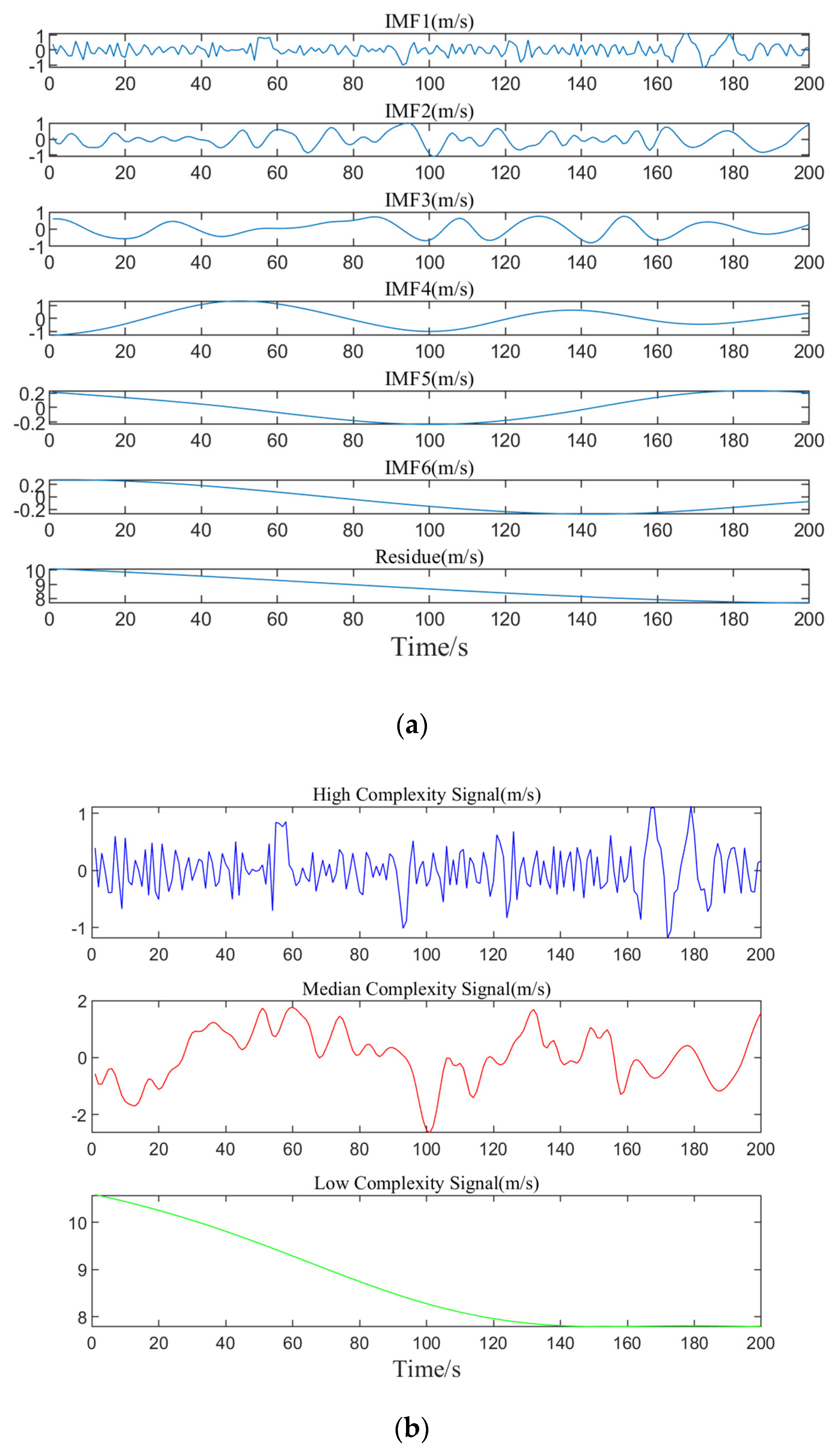
Figure 5a, it can be seen that through the EMD method, the data are progressively broken down into multiple IMFs and a residual term, revealing the multi-level variation characteristics of the data from high complexity to low complexity, to some extent, from high frequency to low frequency. As the decomposition proceeds, the frequency of the subsequent IMF components gradually decreases, the volatility weakens, and eventually tends to be stable, demonstrating the change process of the data ranging from high to low frequencies.
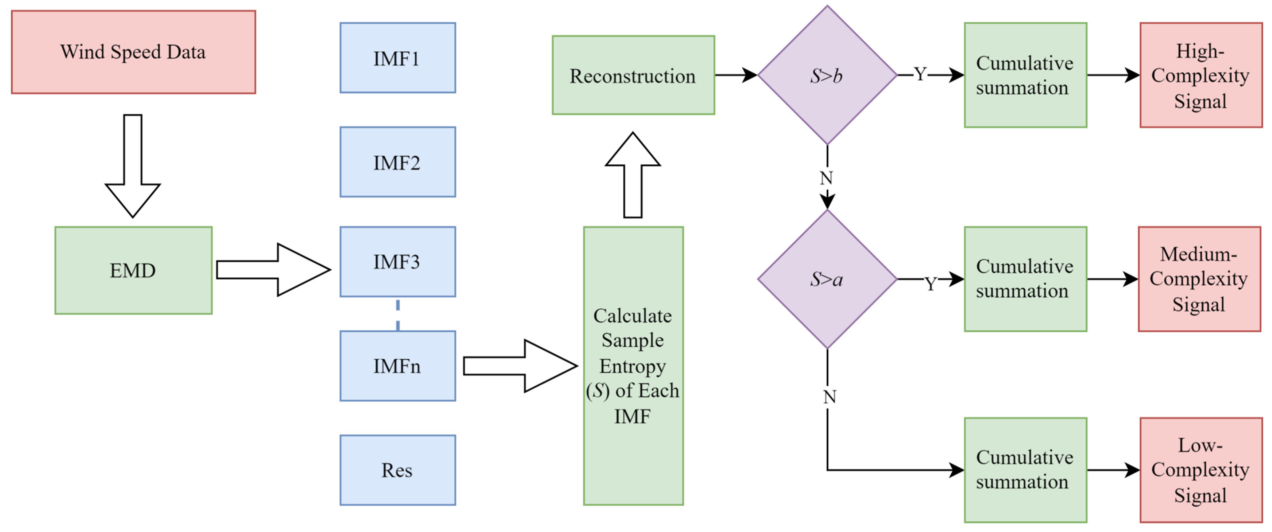
Figure 5b shows that the merged components are categorized into high, medium, and low-frequency ranges, each showing different fluctuation trends. By analyzing these three frequency components, the model’s feature input is simplified, which more accurately captures the signal’s change trend in the prediction model, thus enhancing the model’s predictive accuracy.
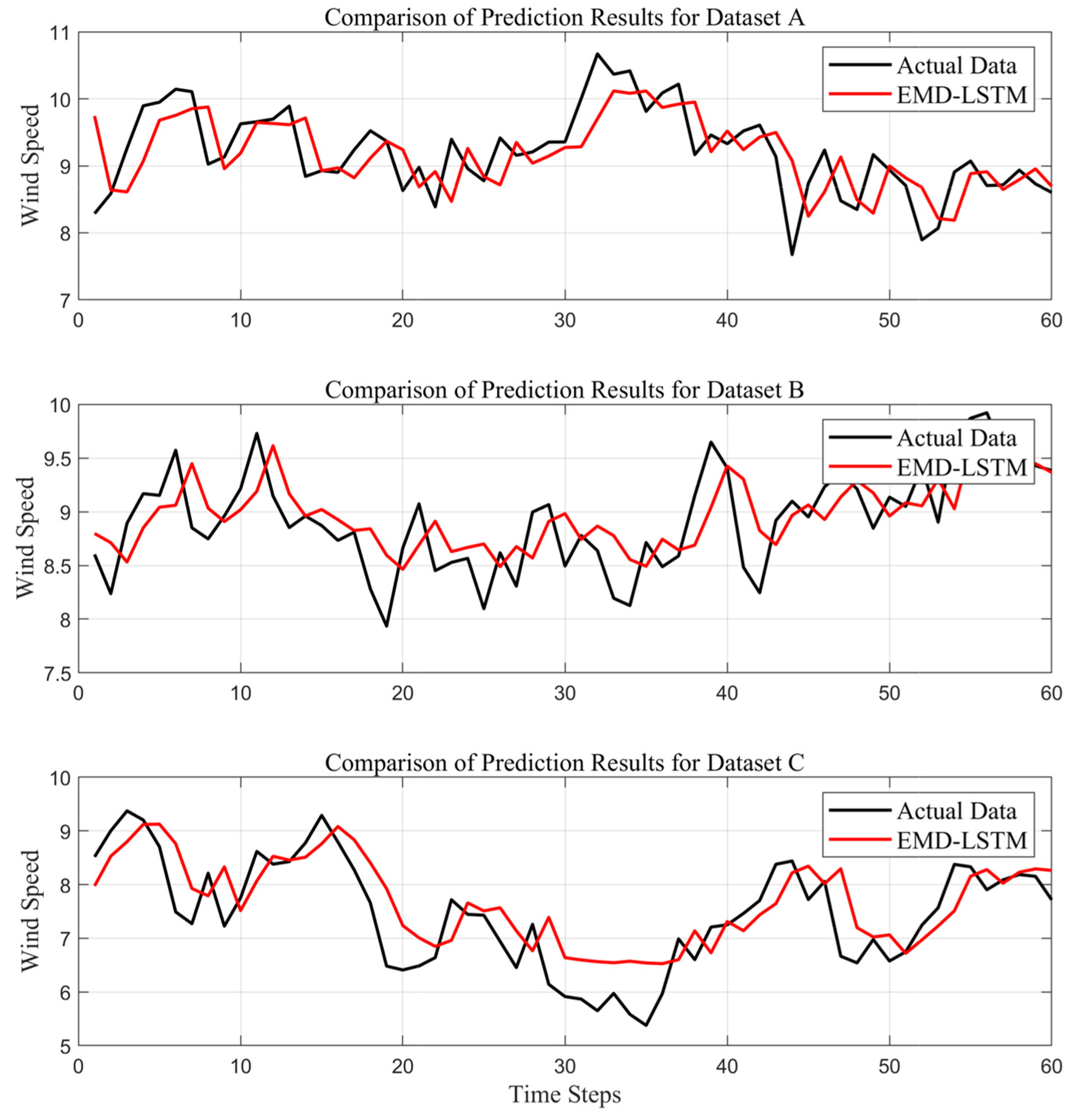
To assess the forecasting performance of the EMD-LSTM model across different datasets, single-step wind speed prediction experiments were conducted using datasets A, B, and C. According to the rolling decomposition–synthesis–forecasting steps, the data rolling window size is set to 200 (i.e., using 200 historical samples of wind speed to predict the next data point), and the data are divided into 1800 groups, using the first 1740 data samples for training and the final 60 samples for testing. The experiments are conducted under the same model parameters, and the forecasting outcomes of the test sets for different groups of data are plotted as shown in
Figure 6.
Comparing the trend in wind speed prediction results for different datasets, all prediction curves have essentially captured the variation trend of the actual values. However, it is evident that the prediction results for dataset B are the best, with the model effectively capturing the rising and falling fluctuation trends in the data.
To more quantitatively evaluate the model’s predictive performance, the model’s strengths and weaknesses are evaluated by analyzing its performance across different experimental datasets using a range of evaluation metrics. The evaluation metrics for each model, including MAPE, MAE, and RMSE, are listed in
Table 2. These metrics can help explain the model’s predictive accuracy, thereby better selecting a model suitable for wind speed prediction.
Based on the defined evaluation metrics, a comparative analysis of the prediction model performance for datasets A, B, and C is conducted. The analysis reveals that dataset B yields the best performance, achieving 0.2921 m/s for MAE, 3.3151% for MAPE, and 0.3566 m/s for RMSE. The difference between its forecasts and the true value is minimized, and its accuracy is the highest. The prediction performance of dataset A is also relatively good, with all metrics slightly higher than those of dataset B. However, dataset C has the worst prediction performance. The MAE, MAPE, and RMSE values for this dataset stand at 0.5165 m/s, 7.3877%, and 0.6320 m/s, showing a notable increase compared to the other two datasets. This may reflect the higher complexity inherent in dataset C. Overall, for these three datasets, the prediction errors are relatively small, suggesting that the model demonstrates strong stability.
(2) Prediction Error Analysis
To further analyze the prediction errors of the proposed EMD-LSTM, the key statistical metrics, i.e., maximum, minimum, mean, median, and standard deviation, are calculated. The results for the different datasets are shown in
Table 3.
As shown in
Table 3, in terms of maximum and minimum errors, Dataset A has a maximum error of 0.9684 m/s and a minimum error of −1.4543 m/s, while Dataset C has a maximum error of 0.8648 m/s and a minimum error of −1.6303 m/s. Compared to Dataset B, which has a maximum error of 0.6922 m/s and a minimum error of −0.8200 m/s, both Datasets A and C exhibit larger negative error extremes. This indicates that, across the three datasets, the model’s predictions for Datasets A and C are slightly lower than the true values at certain time points. This discrepancy may stem from anomalous fluctuations in wind speed data, which the model struggles to capture accurately.
Regarding mean errors, Dataset A has a mean error of 0.0452 m/s, slightly above zero, suggesting that predictions are marginally higher than true values on average. Dataset B has a mean error of −0.0481 m/s, slightly below zero, indicating that predictions are marginally lower than true values. Dataset C, however, shows a larger negative mean error of −0.2125 m/s, reflecting a consistent underprediction by the model.
In terms of standard errors, Dataset A has a standard error of 0.5172 m/s, Dataset B 0.3564 m/s, and Dataset C 0.6003 m/s. Dataset B’s smaller standard error indicates a more concentrated error distribution and better model stability. In contrast, the larger standard errors of Datasets A and C suggest higher error dispersion and poorer prediction stability. This is likely attributable to the more complex and variable wind speed patterns in Datasets A and C, making it challenging for the model to achieve accurate fitting and resulting in increased error variability.
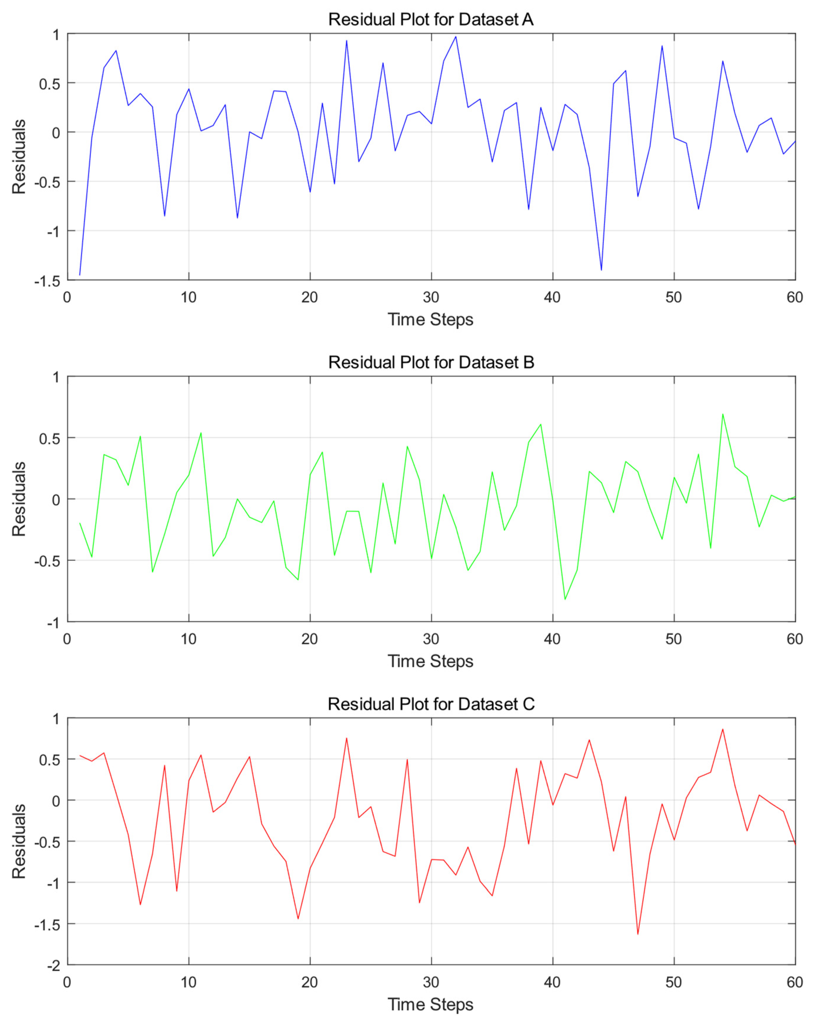
Additionally, the errors are visualized through residual plots illustrated in
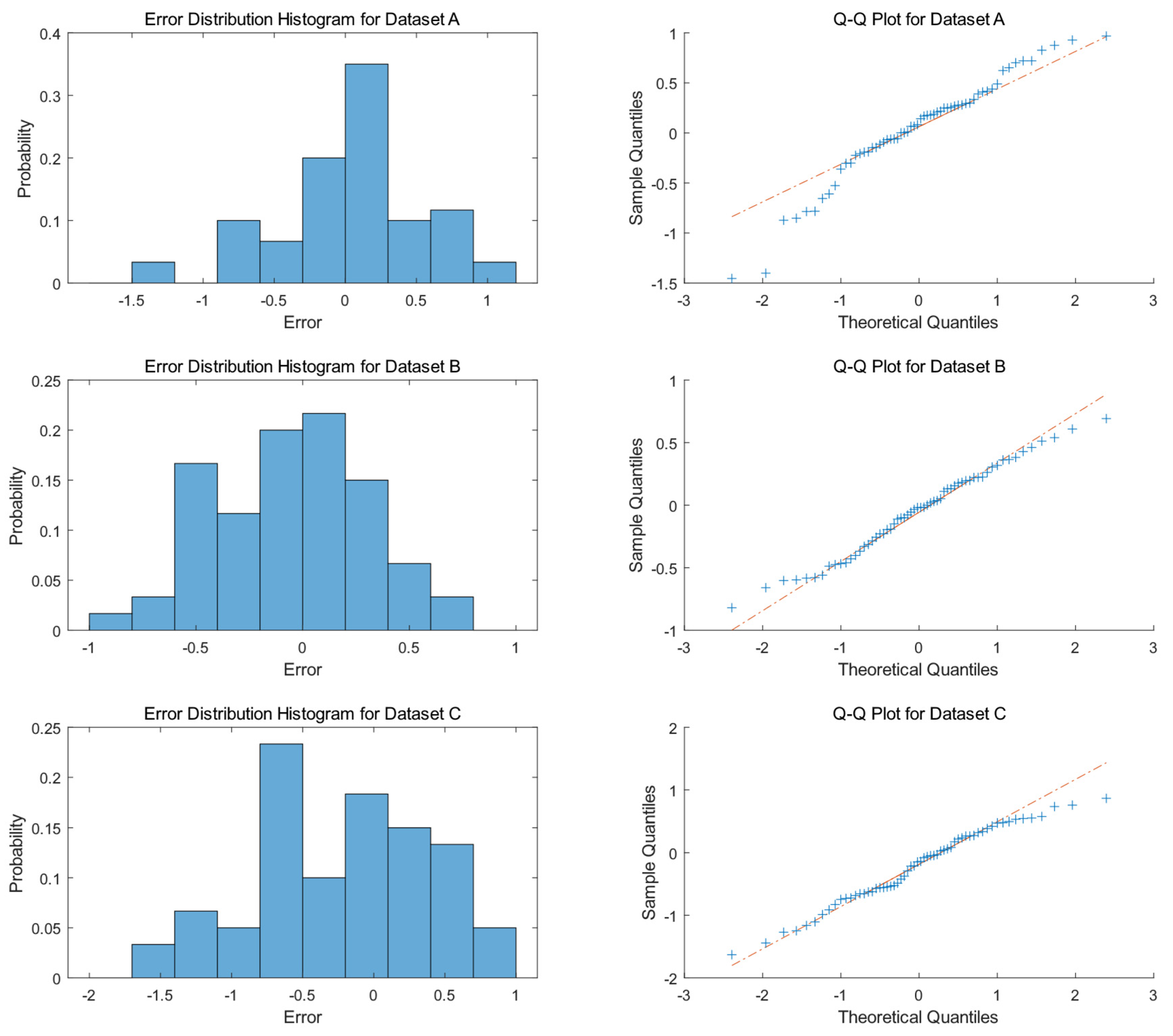
Figure 7 and error distribution histograms and Q-Q plots illustrated in
Figure 8 to further investigate the underlying causes of the model’s prediction errors.
Figure 7 clearly shows that the residuals of Dataset A exhibit frequent and significant fluctuations, ranging between −1.5 and 1, with multiple peaks and troughs. This indicates substantial deviations between the model’s predictions and actual values at these time steps. Moreover, the residuals lack a discernible pattern, showing no clear periodic fluctuations or consistent trend lines, and are randomly distributed around zero. In contrast, the residuals of Dataset B demonstrate relatively milder fluctuations, generally within the range of −1 to 1. While appearing random, their distribution around zero is uneven, with varying degrees of deviation across different intervals. Dataset C exhibits even wider residual fluctuations, with some time steps approaching −2, highlighting more pronounced deviations between predicted and actual values. The residuals show no apparent pattern and are chaotically distributed across the axis. Overall, the residuals of all three datasets deviate from the ideal state of random distribution. This phenomenon is closely tied to the stochastic and complex nature of wind speed sequences. The inherent uncertainty and complexity of wind speed make it challenging for the model to accurately capture its variations, resulting in residuals that fail to conform to an ideal random distribution.
The histogram illustrated in
Figure 8 reveals that the prediction errors of Dataset A are predominantly concentrated between −1 and 1, with a peak near 0, exhibiting a probability of approximately 35%. A minor distribution is observed around −1.5, though with a probability of less than 5%. Thus, the error distribution of Dataset A is basically symmetric, with limited instances of under-prediction. Dataset B demonstrates a relatively symmetric error distribution, with errors uniformly distributed between −1 and 1, showing more balanced probabilities across error intervals compared to Dataset A. Dataset C exhibits a more dispersed error distribution, with higher probabilities for errors between −1 and 0.5, peaking near −0.5. Errors around −2 and 1 also occur, but with lower probabilities. Compared to Datasets A and B, Dataset C shows a higher probability of errors in the negative region, indicating a greater tendency for the model to under-predict on this dataset.
The right column of
Figure 8 illustrates the Q-Q plots, which further validate the normality of residuals across different datasets. For Dataset A, the data points do not strictly align with the theoretical line on the Q-Q plot, particularly deviating at the tails, especially on the left side, indicating that its residual distribution differs from a normal distribution and does not satisfy the normality assumption. Dataset B’s data points closely cluster around the theoretical line, suggesting that the sample quantiles closely match the theoretical quantiles, implying that its residual distribution is relatively similar to a normal distribution. In Dataset C’s Q-Q plot, the data points exhibit significant deviations from the theoretical line, particularly in the middle section, indicating a substantial divergence of its residual distribution from the theoretical normal distribution model.
In summary, the error distributions of the EMD-LSTM model vary across different datasets. Dataset B’s error distribution is closest to a normal distribution, indicating relatively better predictive performance of the model. In contrast, the error distributions of Datasets A and C exhibit varying degrees of deviation from normality.
(3) Data Leakage Analysis
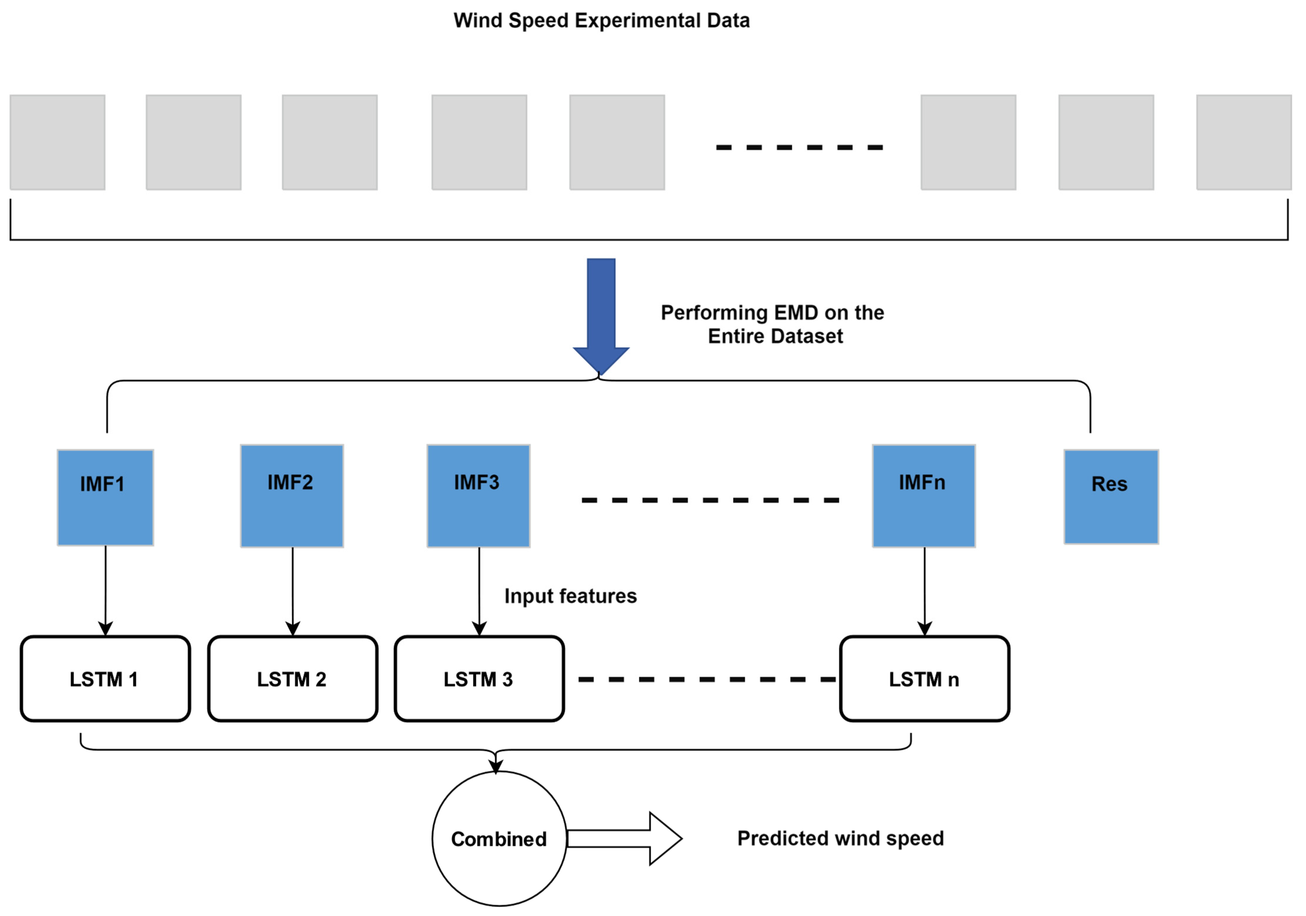
From a methodological perspective, the traditional EMD approach carries the risk of information leakage. The conventional method involves performing EMD on the entire dataset to obtain all IMF components before dividing the data into training and test sets. Since the IMF components are derived from the overall trend of the original wind speed sequence, the training set inadvertently gains knowledge of the test set’s fluctuation trends during model training. This leads to artificially inflated prediction accuracy on the test set, failing to reflect the model’s true predictive capability.
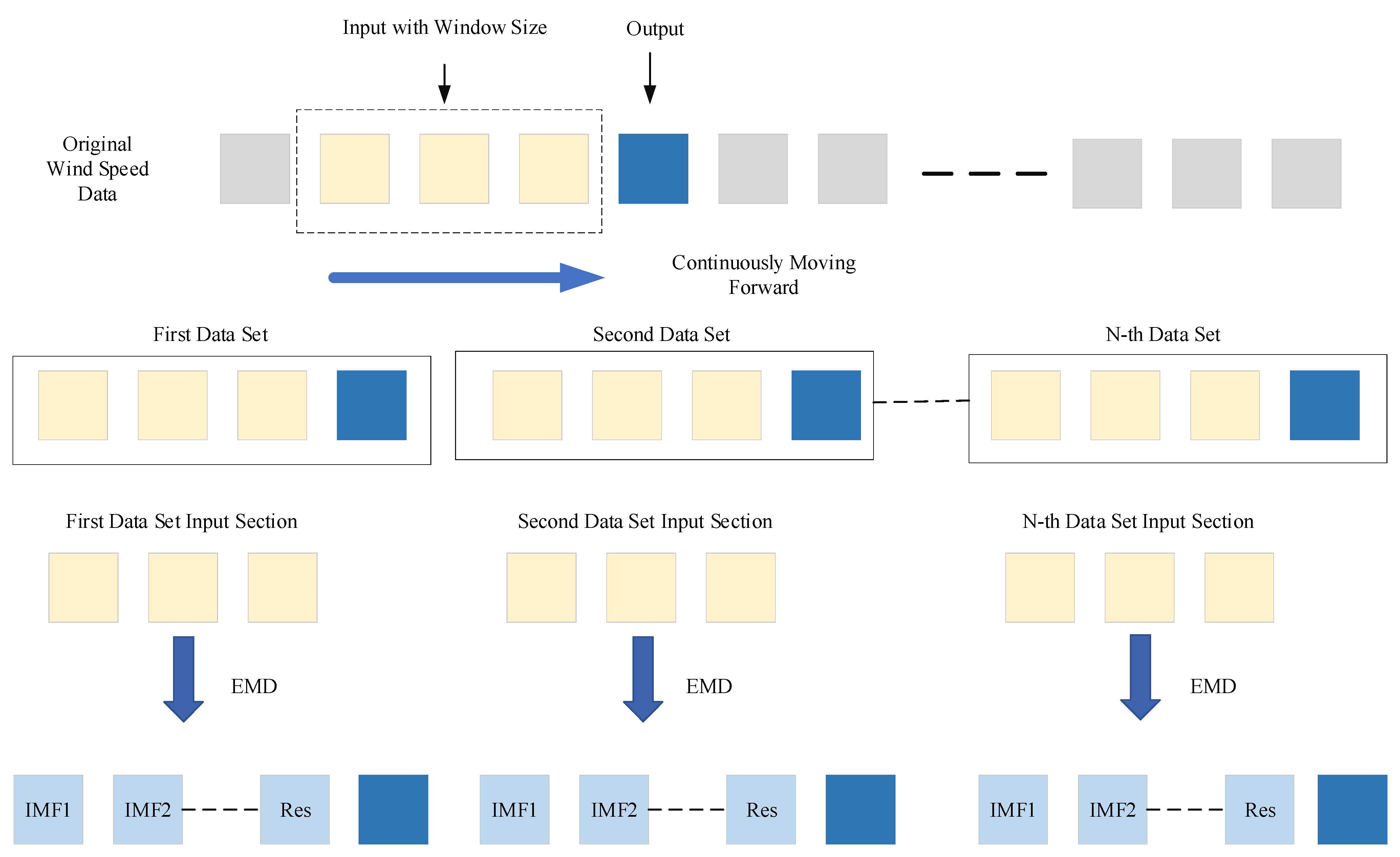
In contrast, the rolling EMD method proposed in this study effectively addresses this issue at its core. The method begins by dividing the data into multiple input–output pairs based on a specific rolling window size. Subsequently, the input data undergo decomposition and reconstruction as described in the paper, yielding three feature-rich components that correspond one-to-one with the output. These input–output pairs are then divided into training, validation, and test sets, followed by model training and prediction. During the training phase, the inputs consist of the three decomposed components derived solely from historical records within the rolling window, ensuring that only past wind speed information is utilized. The output during training is the data for the next time step, which are pre-divided and do not participate in the decomposition process. This ensures that the model does not gain access to any future information during training, fundamentally preventing information leakage. During the prediction phase, once the model is trained and begins predicting on the test set, the test set data remain entirely independent of the training process. The model can only rely on the knowledge acquired during training to make predictions, free from interference by other data sources. This approach guarantees the authenticity and reliability of the prediction results.
(4) Potential for Practical Applications
In practical wind speed prediction scenarios, the trained EMD-LSTM model may run through a systematic process to predict wind speeds at each time step. Specifically, for predicting the wind speed at time step T, the model first retrieves historical wind speed data within a predefined rolling window prior to time T. These data are then subjected to Empirical Mode Decomposition (EMD), which breaks them down into multiple Intrinsic Mode Functions (IMFs). These IMFs are subsequently reconstructed into three distinct frequency-specific components using the sample entropy method. The LSTM network leverages these three components to perform a detailed prediction analysis, ultimately generating the predicted wind speed value for time T. Once this prediction is completed, the model shifts its focus to predicting the wind speed for the next time step, T + 1. At this stage, the model integrates the actual wind speed data newly updated at time T into the rolling window. To maintain a consistent window size, the oldest data point is removed, ensuring computational stability and consistency throughout the process. Following the data update, the model reapplies EMD to decompose the newly updated rolling window data and reconstructs them using the sample entropy method. The LSTM network then utilizes these newly generated components to predict the wind speed for time T + 1. This continuous rolling prediction mechanism ensures that the output data do not participate in the decomposition process, thereby eliminating any risk of information leakage. This approach guarantees the authenticity and reliability of the prediction results, making the EMD-LSTM model a robust tool for practical wind speed prediction applications.
4.4. Parameter Analysis
(1) Sample Entropy Parameters
To investigate the effects of different combinations of sample entropy parameters
m and
r on the prediction performance of the EMD-LSTM model, a sensitivity analysis is performed. In this experiment, the key parameters of sample entropy are systematically defined and varied, with
m taking values of [1, 2, 3] and
r taking values of [0.1, 0.15, 0.2, 0.25]. These parameter combinations are comprehensively tested across three different datasets to provide an in-depth analysis of how variations in sample entropy parameters affect the prediction results of the EMD-LSTM model. The prediction results of EMD-LSTM with different sample entropy parameter combinations are presented in
Table 4,
Table 5 and
Table 6 for various datasets.
From
Table 4, for Dataset A, when
m = 1, as
r increases, the MAE, RMSE, and MAPE first increase and then decrease, with small fluctuations. When
m = 2, the changes in the indicators are more complex, with the RMSE reaching a relatively low value when
r = 0.2. For
m = 3, the indicators show a relatively slow overall change, but the values are higher. It can be observed that in Dataset A, different parameter combinations affect model performance, with the combination of
m = 2 and
r = 0.2 performing best according to the indicators.
From
Table 5, for Dataset B, when
m = 1, the differences in the indicators for different parameter combinations are significant, especially when
r = 0.15, where all error metrics are noticeably high. When
m = 2, the indicators remain relatively stable as
r changes, and the overall values are lower. For
m = 3, there is some fluctuation in the indicators. This suggests that in Dataset B, the parameter setting of
m = 2 leads to a more stable model performance, with the combination of
m = 2 and
r = 0.2 yielding the lowest error metrics and the best prediction performance.
From
Table 6, for Dataset C, when
m = 1, the error indicators fluctuate significantly as r changes. For
m = 2, when
r = 0.15, both MAE and RMSE are relatively small, while MAPE remains within a reasonable range when
r = 0.2. For
m = 3, the indicators exhibit a wider range of variation. Overall, for Dataset C, the model performs best with
m = 2, showing good adaptability to different values of
r, with the combination of
m = 2 and
r = 0.2 achieving a good balance across the evaluation metrics.
Based on the analysis of these three datasets, selecting the sample entropy parameters m = 2 and r = 0.2 consistently leads to the best and most balanced results across all evaluation metrics.
(2) Component Reconstruction Threshold Parameters
With the sample entropy parameters fixed at
m = 2 and
r = 0.2, a sensitivity analysis is conducted to explore the impact of different component merging threshold parameter combinations on the prediction performance of the EMD-LSTM model. In the experiment, a series of threshold combinations are defined, specifically [mid-frequency and low-frequency threshold
a, mid-frequency and high-frequency threshold
b], with the following values: [0.05, 0.5]; [0.1, 0.6]; [0.15, 0.7]; [0.2, 0.8]. These key parameters are systematically varied, and the model’s prediction performance is comprehensively tested. The prediction results of this experiment with various threshold parameter combinations for different datasets are presented in
Table 7,
Table 8 and
Table 9.
From the model prediction results for Datasets A, B, and C as seen in
Table 7,
Table 8 and
Table 9, respectively, it is evident that different threshold parameter combinations have varying impacts on the evaluation metrics. In Dataset A, the fluctuations in the indicators are relatively small as the parameters change, with
a = 0.15 and
b = 0.70 yielding the best performance in RMSE. In Dataset B, when
a = 0.1 and
b = 0.6, all three-evaluation metrics reach their lowest values, indicating outstanding prediction accuracy. In Dataset C, the indicator fluctuations are more stable, with
a = 0.2 and
b = 0.8 yielding a relatively low MAPE.
Overall, although the parameter combination a = 0.1 and b = 0.6 does not achieve the lowest values for all metrics in every dataset, it performs well across the board in terms of overall prediction accuracy, particularly excelling in Dataset B. Therefore, the combination of a = 0.1 and b = 0.6 is selected as the threshold for component merging.
4.5. Comparisons with Other Methods
To comprehensively validate the performance of the proposed model, comparative experiments are conducted between the EMD-LSTM model and other wind speed prediction methods, including SVM, ARIMA, GRU, and LSTM, across the three datasets. All experiments are carried out under the same experimental conditions, using the same datasets and evaluation metrics to ensure consistency.
Experimental Setup: The experiments are conducted on a desktop computing platform with an Intel(R) i7-10700K CPU, 16 GB of RAM, and Matlab 2024b software environment, where the model construction, training, and validation are systematically carried out.
Model Parameter Settings: For the ARIMA model, the parameters are set as (p, d, q) = (3, 1, 2). The SVM model utilizes a Gaussian kernel with automatic scale adjustment. The GRU and LSTM models have identical parameters: the Adam algorithm as the optimizer, a maximum of 50 iterations, an initial learning rate of 0.004, a learning rate decay factor of 0.5 every 20 iterations, and a minimum batch size of 64. The EMD-LSTM model uses sample entropy parameters m = 2, r = 0.2, and component merging thresholds of (0.1, 0.6).
(1) Prediction Accuracy
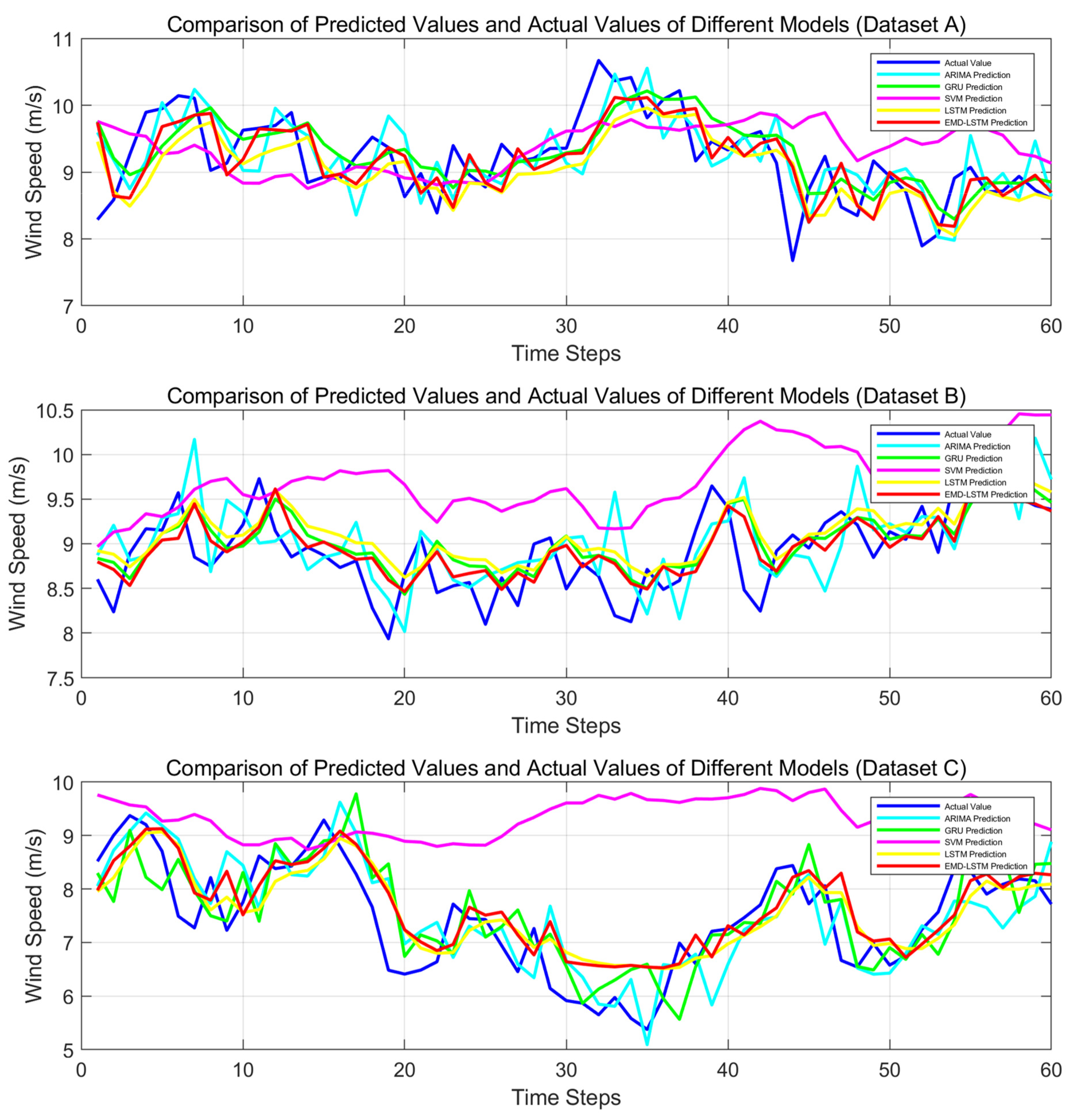
The prediction curves for different method combinations are plotted as shown in
Figure 9. It can be clearly observed from this figure that in Dataset A, the prediction curves of all models fluctuate frequently, with the EMD-LSTM model’s curve being relatively closer to the actual value curve, effectively capturing the wind speed variation trend. In Dataset B, the models show varied performance, with some models exhibiting significant deviations in their prediction curves. However, the EMD-LSTM model has a smaller deviation from the actual values at most time steps, and its fluctuations closely mirror the variations in actual wind speed. In Dataset C, in the face of complex wind speed changes, the EMD-LSTM model’s prediction curve follows the actual values more closely than the other models, showing a higher degree of alignment at key wind speed change points.
Overall, across all three datasets, while each model reflects wind speed changes to some extent, the EMD-LSTM model demonstrates superior performance with a higher degree of alignment between its prediction curve and the actual value curve, as well as better consistency in fluctuation trends. This indicates its stronger ability to capture wind speed variation characteristics and its higher prediction accuracy, outperforming the other comparison models.
By analyzing the model’s performance across different datasets using a variety of evaluation criteria, the superiority or inferiority of the models can be assessed. The evaluation metrics, including MAE, MAPE, and RMSE, are listed in
Table 10,
Table 11 and
Table 12, respectively, for various models on different datasets.
From the above
Table 10,
Table 11 and
Table 12, it can be observed that in Dataset A, compared to the LSTM model, the EMD-LSTM model achieves a reduction of approximately 11.46% in MAE and 7.97% in RMSE. While MAPE remains the same, the former two metrics demonstrate superior performance. When compared to other models, the ARIMA and SVM models have significantly higher error metrics than EMD-LSTM, while the GRU model shows some similarity in certain indicators, but overall, EMD-LSTM controls errors more effectively. In Dataset B, the EMD-LSTM model reduces MAE by approximately 14.44%, RMSE by 13.89%, and MAPE by 15.07% compared to the LSTM model, showing a significant improvement in prediction accuracy. In comparison to other models, SVM exhibits much higher error metrics than EMD-LSTM. ARIMA and GRU models are competitive but still lag behind the EMD-LSTM model. In Dataset C, the EMD-LSTM model reduces MAE by approximately 5.40%, RMSE by 2.56%, and MAPE by 3.92% compared to the LSTM model, achieving better prediction accuracy. Compared to other models, SVM has the largest error, and both ARIMA and GRU models have higher error metrics than EMD-LSTM.
Considering the evaluation across all three datasets, the EMD-LSTM model shows a significant reduction in MAE, RMSE, and MAPE compared to the other models, especially the LSTM model, indicating superior prediction performance.
(2) Model Complexity Analysis
In addition to focusing on prediction accuracy, computational complexity is also a critical consideration, as it directly affects the efficiency and feasibility of the model in practical applications. Here, the time spent in the prediction stage of various models in the same computer environment is used as the alternative indicator to represent computational complexity. The time consumption of ARIMA, GRU, SVM, LSTM, and the proposed EMD-LSTM during the prediction phase is shown in
Table 13.
From the perspective of time consumption during the prediction phase shown in
Table 13, the computational complexity of different models shows little variation across datasets. The SVM model has the shortest prediction time on Datasets A, B, and C, indicating higher computational efficiency and relatively lower complexity during the prediction phase. The GRU model also has a shorter prediction time, placing its computational complexity at a relatively low level. The time consumption of the LSTM and EMD-LSTM models is similar, with both models exhibiting comparable computational complexity across the three datasets. In contrast, the ARIMA model shows significantly higher prediction time on all three datasets compared to the other models. EMD-LSTM, as a newly proposed method, has a prediction stage time consumption of approximately 0.36 s across these three datasets, which is comparable to GRU and LSTM, slightly higher than SVM (approximately 0.12–0.21 s), but significantly lower than ARIMA (approximately 1.2–1.3 s). This indicates that EMD-LSTM outperforms ARIMA in efficiency and approaches GRU and LSTM, but is slightly inferior to SVM. The advantage of EMD-LSTM likely lies in its combination of EMD (Empirical Mode Decomposition) and LSTM, enabling it to better capture multi-scale features in complex time series, making it suitable for nonlinear and non-stationary data prediction tasks. Although its computational time is slightly longer than that of GRU and LSTM, it remains suitable for practical applications and shows greater potential in accuracy and feature extraction capabilities.
4.6. Statistical Analysis and Nonparametric Test
(1) Statistical Analysis
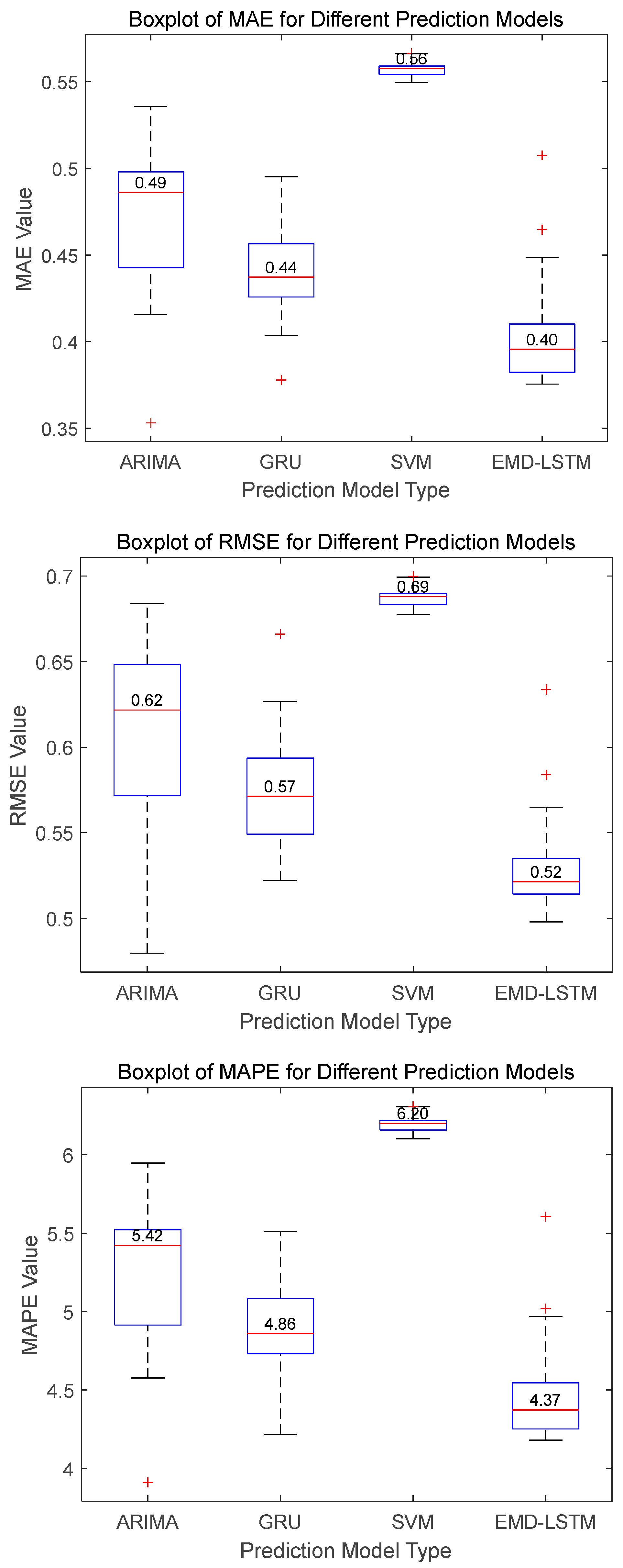
To comprehensively and accurately assess the performance of the proposed EMD-LSTM method compared to other existing models such as ARIMA, SVM, and GRU in wind speed prediction, each of the aforementioned models is run 30 times separately under the same experimental environment and parameter settings. The evaluation metrics of different models are statistically analyzed. Through multiple independent runs and systematic statistical analysis, the performance of each model on different datasets is obtained, and a solid data foundation is provided for comparing their advantages and disadvantages. For Dataset A, the MAE, RMSE, and MAPE values of ARIMA, SVM, GRU, and EMD-LSTM models in 30 runs are obtained; their boxplots are illustrated in
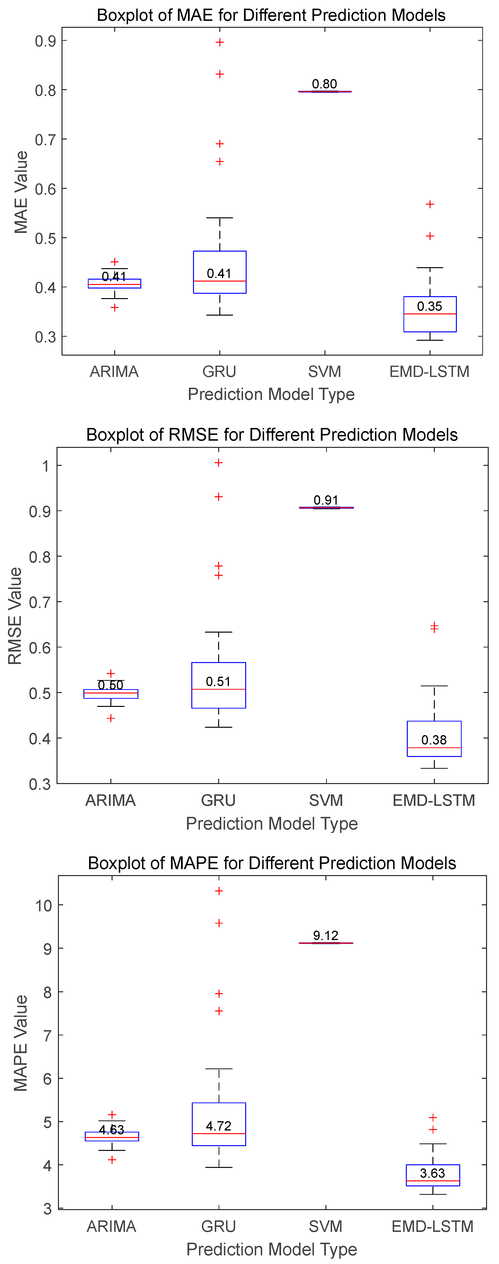
Figure 10. The statistical comparisons of the three metrics for different algorithms on Dataset B and Dataset C are presented in
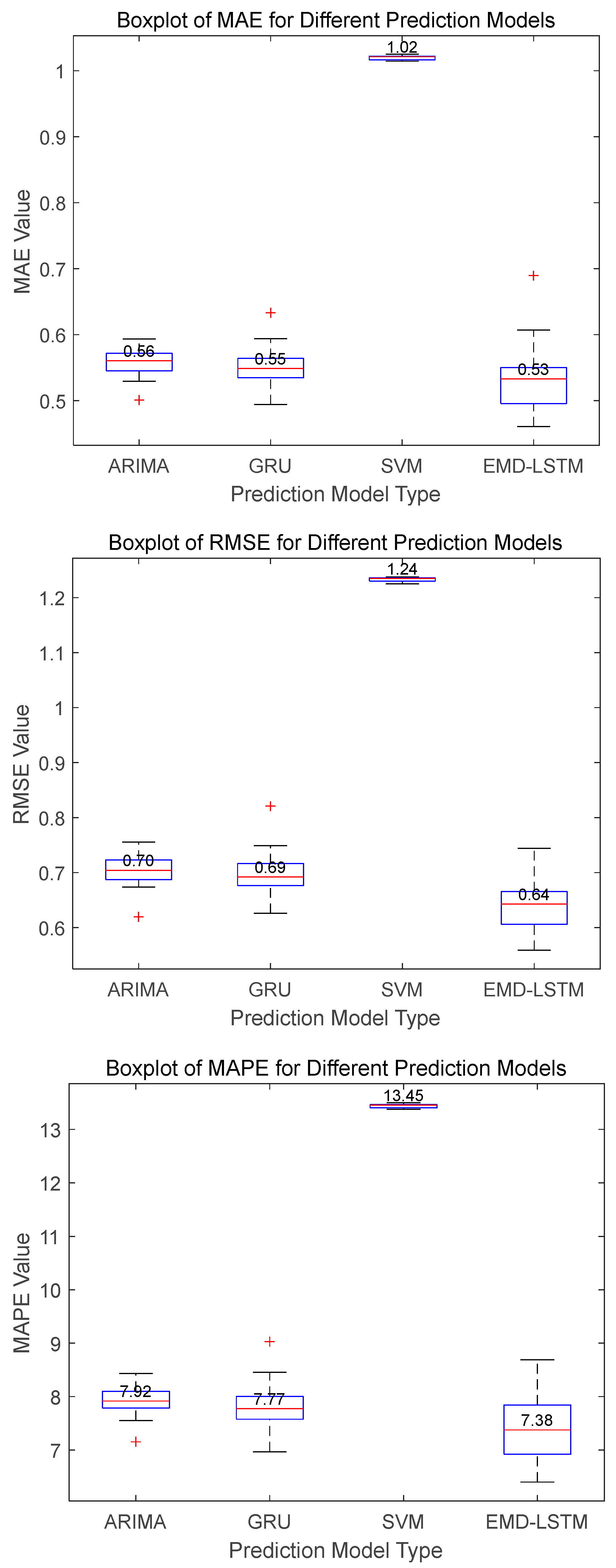
Figure 11 and
Figure 12, respectively.
For Dataset A, the boxplots in
Figure 10 illustrate that the EMD-LSTM model achieves median values of MAE, RMSE, and MAPE at 0.40, 0.52, and 4.37%, respectively, over 30 runs. These figures represent improvements of approximately 9.09%, 8.77%, and 10.08% over the best values obtained by other considered methods, which are 0.44, 0.57, and 4.86%. Furthermore, the EMD-LSTM exhibits a slightly narrower box width compared to ARIMA and GRU, indicating higher stability relative to these methods, while SVM, despite its higher stability, shows significantly higher median values, suggesting lower accuracy than EMD-LSTM. For Dataset B, statistical results shown in
Figure 11 reveal that EMD-LSTM attains median values of MAE, RMSE, and MAPE at 0.35, 0.38, and 3.63%, respectively, over 30 independent runs, marking improvements of 14.63%, 24%, and 21.59% over the best values from other comparative algorithms, which were 0.41, 0.51, and 4.63%. For Dataset C illustrated in
Figure 12, EMD-LSTM achieves median values of MAE, RMSE, and MAPE at 0.53, 0.64, and 7.38%, respectively, over 30 independent runs, outperforming the best values from other comparative algorithms by 3.64%, 7.25%, and 5.02%, which are 0.55, 0.69, and 7.77%. In summary, based on the median values of multiple experimental metrics, the EMD-LSTM method demonstrates improvements of at least 3.64%, 7.25%, and 5.02% over other methods across the considered test datasets.
(2) Nonparametric Test
To further validate the effectiveness of the proposed EMD-LSTM model compared to the other three models, a non-parametric test analysis is conducted. The Wilcoxon test is applied, with the significance level 0.05 as the criterion. The null hypothesis assumes no significant difference between EMD-LSTM and the other models (h = 0), while the alternative hypothesis assumes a significant difference (h = 1). Pairwise comparisons of the EMD-LSTM model with ARIMA, GRU, and SVM are made across the three datasets, using the specified significance level as the threshold. The results of the non-parametric tests for the three datasets are presented in
Table 14,
Table 15 and
Table 16.
The Wilcoxon test results as shown in
Table 14,
Table 15 and
Table 16 for MAE, MAPE, and RMSE across the three datasets show that the
p-values for all models compared to EMD-LSTM are significantly less than 0.05, with h = 1 in all cases. This indicates that, across all datasets and evaluation metrics, there are significant differences in prediction performance between the ARIMA, GRU, SVM models, and the EMD-LSTM model. As previously discussed from the boxplots in
Figure 10,
Figure 11 and
Figure 12, the EMD-LSTM model exhibits lower median values for MAE, RMSE, and MAPE, indicating superior prediction accuracy. These Wilcoxon test results further confirm, from a statistical perspective, that the EMD-LSTM model has a significant advantage over ARIMA, GRU, and SVM models in prediction performance, thereby validating the model’s effectiveness.


