Article

LSTM Model Combined with Rolling Empirical Mode Decomposition and Sample Entropy Reconstruction for Short-Term Wind Speed Forecasting

1
Dongfang Electric Wind Power Co., Ltd., Deyang 618000, China
2
Department of Instrumental and Electrical Engineering, Xiamen University, Xiamen 361005, China
*
Authors to whom correspondence should be addressed.
Processes 2025, 13(3), 819; https://doi.org/10.3390/pr13030819
Submission received: 6 February 2025 / Revised: 1 March 2025 / Accepted: 6 March 2025 / Published: 11 March 2025

Abstract

:
This research introduces a new hybrid forecasting approach based on a rolling decomposition–merging–prediction framework integrating Empirical Mode Decomposition (EMD), sample entropy, and Long Short-Term Memory (LSTM) to further enhance the accuracy of wind speed predictions. To avoid the information leakage issue caused by decomposing wind speed data, a rolling EMD method is applied to the framework to ensure that the data points to be predicted are excluded from the decomposition process. The input speed data of the prediction model are then decomposed into a series of Intrinsic Mode Functions (IMFs) and a residual component, capturing the local variation characteristics of the wind speed data. Next, the sample entropy method is employed to calculate the entropy values of these components, which are then reclassified and aggregated into three components based on their calculated entropy values, corresponding to high, medium, and low frequencies. The three reconstructed components are then employed as input features in an LSTM model for wind speed prediction. To demonstrate the effectiveness of the proposed model, experiments using three different datasets were conducted with wind speed data collected from a wind farm. The statistical experimental results indicate that the proposed EMD-LSTM achieves improvements in metrics of MAE, RMSE, and MAPE by at least 3.64%, 7.25%, and 5.02%, respectively, compared to other methods across the evaluated test datasets. Furthermore, the Wilcoxon test results provide additional evidence, confirming that the EMD-LSTM model exhibits a statistically significant advantage in prediction performance over the ARIMA, GRU, and SVM models.

1. Introduction

The need for energy consistently expands as the economy grows and living standards continue to rise [1]. The reliance on conventional fossil fuels, such as coal and petroleum, has led to significant environmental pollution, ecological damage, and global warming [1]. Wind energy, being a renewable and environmentally friendly resource, has attracted considerable interest. At present, wind energy is an essential component in the development of smart grids, intelligent buildings, and modern homes, playing a crucial role in electricity supply [2]. However, wind speed is influenced by various factors, such as climate change and geographical structures, making wind energy uncertain and volatile. Traditional forecasting methods often struggle to adequately capture the features and variability inherent in wind speed data due to its fluctuating nature. Consequently, developing effective and reliable wind speed prediction methods has emerged as a key focus of research.
Recently, a variety of studies have been conducted globally to explore wind speed forecasting methods. These approaches are typically classified into three main categories: physical, statistical, and artificial intelligence-based methods [3]. Physical methods predict wind speed based on meteorological and topographical information, with the numerical weather prediction method being a commonly used approach [4]. However, physical models typically involve a large number of parameters, which heavily rely on human expertise for adjustment, making it challenging to determine the appropriate parameters for the model. Statistical methods rely on historical data and perform predictions through the analysis of wind speed patterns and statistical trends. Common statistical techniques include time series analysis [5], regression analysis [6], and spectral analysis [7]. However, these methods may perform poorly when dealing with nonlinear relationships, leading to reduced prediction accuracy. General intelligent methods, based on machine learning and artificial intelligence techniques such as artificial neural networks (ANN) [8], support vector machines (SVM) [9], and genetic algorithms (GA) [10] have shown promise in improving forecasting accuracy by uncovering complex patterns and relationships in data. However, these methods often require complex model optimization processes, which can be time-consuming and demand frequent human intervention. As a result, using a single forecasting approach is often insufficient to effectively capture wind velocity variations.
Given the high volatility of wind speed influenced by multiple factors, a “decomposition–prediction” hybrid approach can be employed to enhance wind speed forecasting. Some well-known decomposition techniques such as Wavelet Transform [11], Empirical Mode Decomposition (EMD) [12], and Variational Mode Decomposition (VMD) [13] are widely used in wind speed forecasting. Among these methods, the EMD algorithm utilizes an adaptive decomposition approach, eliminating the necessity of selecting an appropriate basis function. Additionally, in contrast to other decomposition techniques, EMD offers the advantage of faster processing, making it particularly effective for identifying key characteristics in nonlinear and non-stationary signals, which are commonly identified in wind speed data [14]. For instance, Lin L et al. [15] proposed a combined forecasting model based on EMD. In this model, the EMD algorithm was employed to decompose the original wind speed sequence into multiple subsequences, and then these subsequences were modeled and predicted using a support vector regression model optimized by grey wolf optimization algorithm. Similarly, Yang X Y et al. [16] employed EMD to decompose historical wind speed data into components corresponding to different frequency bands. These components were then individually predicted using a weighted Markov Chain, and then the results were summed and subsequently input into a Quantile Regression (QR) model to determine the upper and lower bounds of the wind power probability intervals.
Recently, LSTM, a well-known predictive model, has also incorporated decomposition techniques to provide feature inputs for the neural network. Chen C P et al. [17] introduced a novel forecasting method that improved the technique to extract frequency-specific features from complex wind speed sequences. Ding Y et al. [18] decomposed wind data into crosswind and alongwind speeds considering the correlation between the wind speed and direction. The wind speed and direction data were denoised by EMD and the crosswind and alongwind speeds were predicted using an LSTM model. Nahid F A et al. [19] developed a new multistep hybrid forecasting model for very short-term wind speed forecasts based on data decomposition and a combination of CNN and LSTM algorithms. In their approach, the EMD was employed to transform nonlinear and nonstationary data into relatively simple and stationary subsets. Yan Y et al. [20] proposed a hybrid wind speed prediction model based on seasonal autoregressive integrated moving average (SARIMA), ensemble empirical mode decomposition (EEMD), and long short-term memory (LSTM) methods. In their approach, the characteristics of the wind speed time series were extracted to obtain the trend series, period series, and residual series. Then, the residual series were decomposed into various IMFs and sub-residual sequences, and LSTM was employed to predict these various IMFs and sub-residual sequences. Jaseena K U et al. [21] combined the features of various data decomposition techniques and Bidirectional LSTM networks to forecast wind speed. In their approach, various decomposition techniques such as WT, EMD, EEMD, and EWT were employed to denoise the wind speed data by partitioning the data into low and high-frequency signals.
The aforementioned combined approaches employed decomposition techniques to extract frequency-specific features from complex wind speed sequences while LSTM neural network models were usually constructed to predict these frequency components, and the ultimate wind speed prediction was derived by combining the individual forecasts. Generally, the entire experimental dataset is employed using EMD or similar techniques, thereby including the predicted data within the decomposition process. However, this decomposition method has a major drawback: the decomposed components inadvertently incorporate future wind speed fluctuations, resulting in information leakage and artificially inflated prediction accuracy. Furthermore, since future data are unavailable in real-world wind speed forecasting scenarios, this method, which depends on future data for decomposition, is not practically feasible. To fill this technical gap, this research presents an improved EMD-LSTM model founded on a rolling decomposition–merging–prediction framework to enhance wind speed forecasting accuracy. The model introduces a rolling decomposition method to ensure that the data points to be predicted are excluded from the decomposition process. Additionally, to resolve the misalignment of the number of IMFs across different data groups resulting from the decomposition process, sample entropy [22] is introduced as a key technology to combine the decomposed components into three signals, which are then used as input features for LSTM prediction.
The remainder of the paper is arranged as follows. In Section 2, the traditional LSTM-based wind speed prediction with EMD is briefly reviewed. In Section 3, a detailed description of the LSTM model combined with rolling EMD and sample entropy reconstruction for forecasting wind speed is fully described. The proposed model’s validity is confirmed using a case study and analysis in Section 4. Section 5 presents the conclusions of this research.

2. Traditional LSTM-Based Wind Speed Prediction with EMD

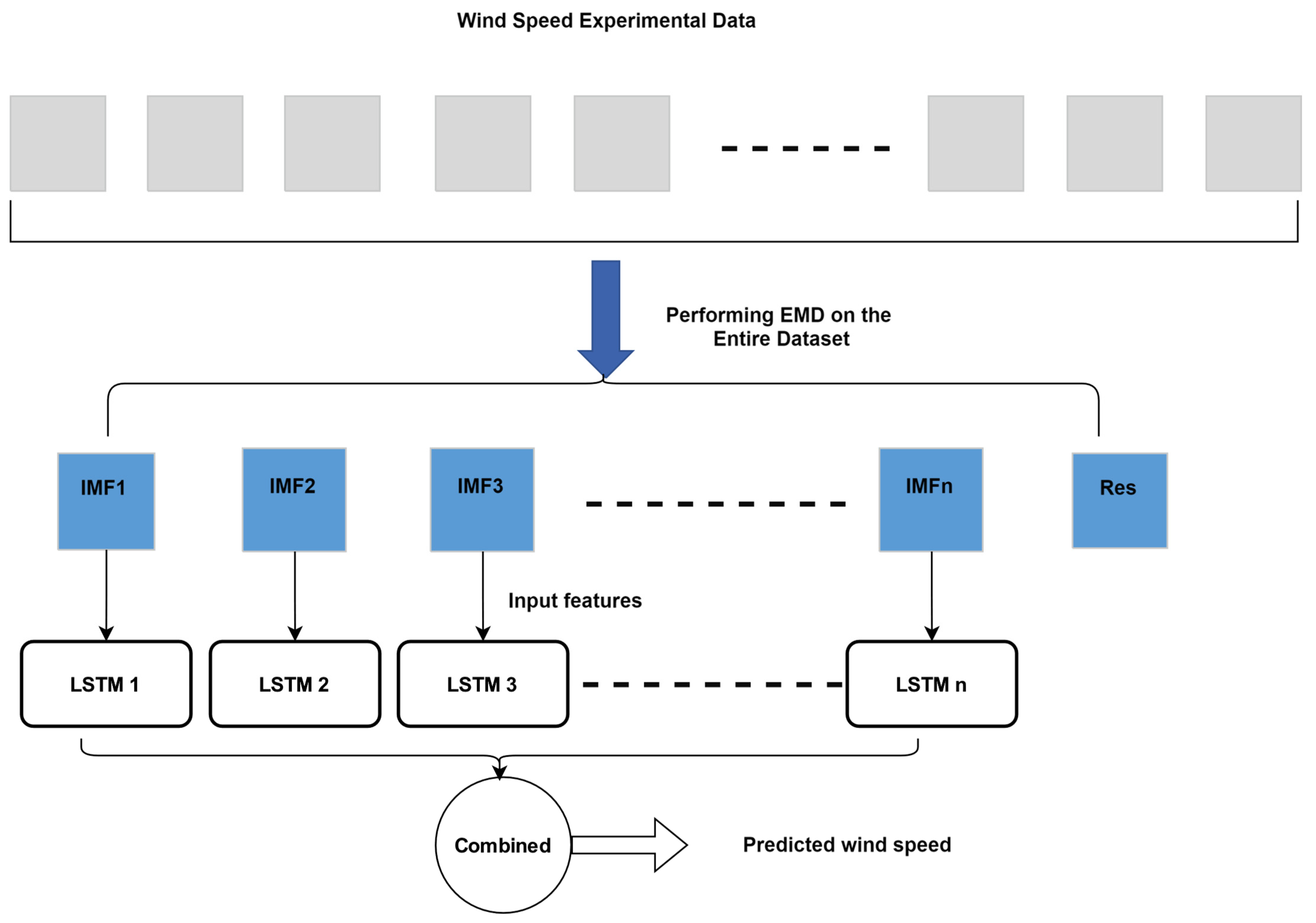
In wind speed forecasting, integrating data decomposition techniques with neural network models is a commonly used approach for improving prediction accuracy. In such methods, the EMD and LSTM combination is one of the most typical hybrid prediction techniques [23]. This method involves several key stages: Firstly, the input wind speed data are preprocessed, consisting of pinpointing and handling potential anomalies and missing values to ensure data quality and accuracy. Next, EMD is used to break down the preprocessed wind speed series into components with varying frequencies, allowing better capture of the local characteristics and variation trends of the wind speed dataset. Then comes the process of model creation, where each decomposed component of the data is fed into the forecasting model for prediction. Generally, an LSTM model is trained using the training dataset to establish a predictive framework for wind speed. In the prediction phase, the trained LSTM model is implemented in the actual wind speed data to forecast each element. Ultimately, the forecasts of all individual components are combined to produce the final wind speed prediction. The complete forecasting procedure is described below, with the specific data decomposition process illustrated in Figure 1.
Step 1: Obtain historical wind speed time series data from wind speed sensors or meteorological monitoring platforms and preprocess the data to ensure their completeness and integrity.
Step 2: Apply the EMD method to partition the preprocessed data into multiple IMFs and a residual component. The dataset is categorized into two groups: 80% or other percentage of the sample is allocated for training the model, while the remaining is reserved for testing.
Step 3: During the model development stage, use the decomposed IMFs and residual components as inputs to the LSTM model. Train separate LSTM models for each component using the training dataset.
Step 4: In the prediction phase, use the trained LSTM models to predict the future values of each IMF and the residual component. Combine the forecasts from all elements to produce the final wind speed prediction.
Step 5: Evaluate the model’s forecasting performance by utilizing standard evaluation measures.
This systematic approach leverages the strengths of Empirical Mode Decomposition (EMD) in capturing local data features and the power of Long Short-Term Memory (LSTM) networks in modeling time-series data, enabling accurate and reliable wind speed forecasting. However, while the decomposition process significantly enhances prediction accuracy, it also introduces the challenge of information leakage when using the EMD-LSTM hybrid model for wind speed forecasting. As shown in Figure 1, the EMD method decomposes the entire wind speed time series, including the data for the prediction period. This implies that during the model training phase, future wind speed information is already utilized, leading to a “pre-knowledge” effect on the test data. As a consequence, the model’s prediction performance appears artificially inflated. This premature exposure of information poses limitations in practical applications, as future wind speed data are unknown in real-world forecasting scenarios and thus cannot be decomposed a priori. This issue highlights the need for alternative approaches that can avoid such information leakage while maintaining high forecasting accuracy.

3. LSTM Model Combined with Rolling EMD and Sample Entropy Reconstruction for Wind Speed Forecasting

3.1. Rolling EMD for Wind Speed Prediction

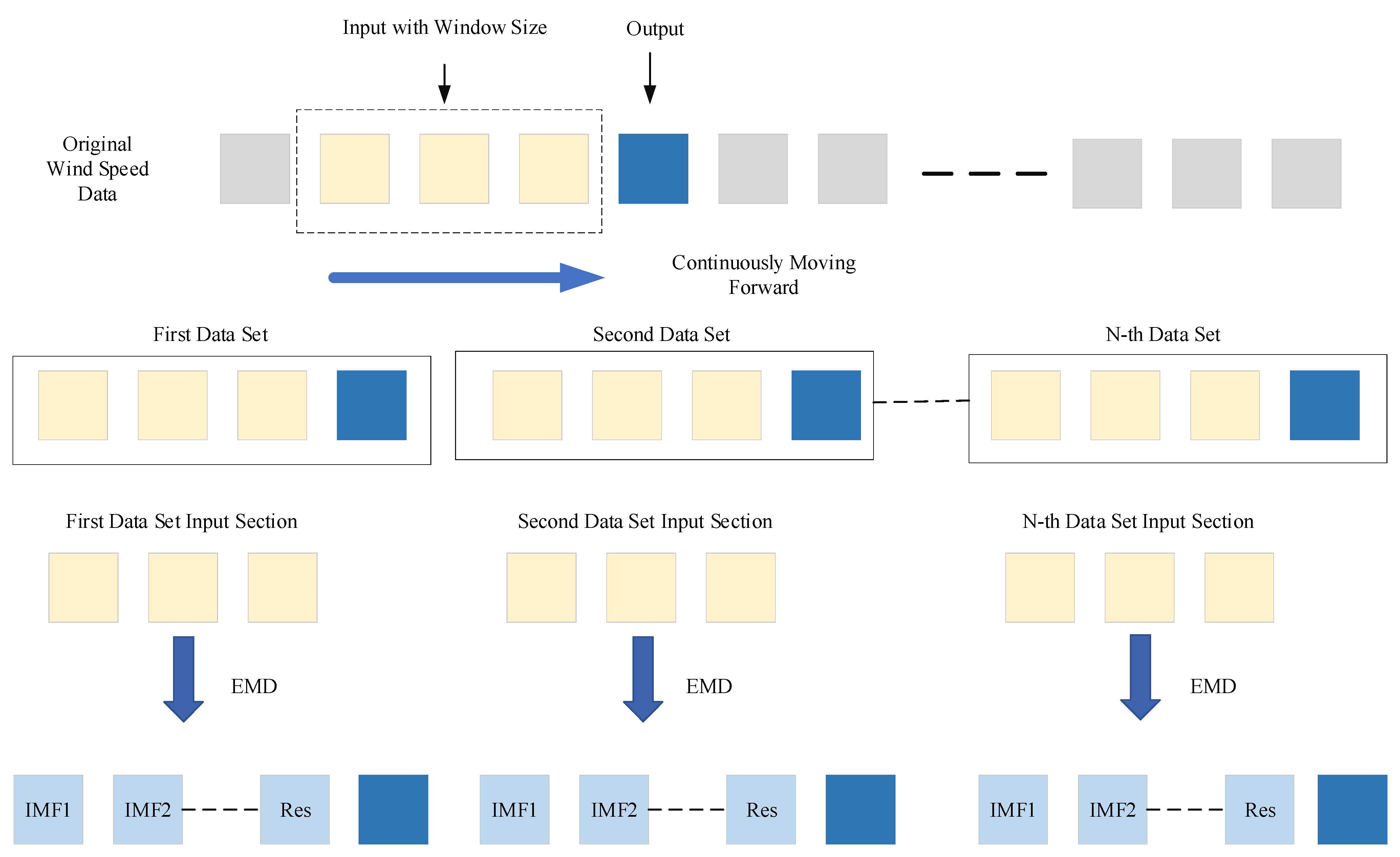
In real-world applications of wind speed prediction, the test dataset is inherently unknown, making it impossible to directly decompose unknown data. This limitation renders many previous research findings impractical for real-world applications. Similarly, when using EMD for forecasting, the problem of data leakage emerges in this context, as the decomposition of test data introduces unknown information into the training process. This results in artificially inflated prediction accuracy for the model [24]. To address this issue, a rolling decomposition method is introduced to avoid information leakage during decomposition. Given that forecasting problems inherently assume the output data are unknown, the decomposition model must not include the unknown data in the decomposition process. Specifically, in the rolling decomposition method, a data window is first defined, with its size determined empirically. Then, the known time series data are divided into input and output subsets based on the window size. Since this is a single-step forecasting problem, each output corresponds to one data point. The input data within the window are subjected to EMD, while the output data are excluded from the decomposition process. The detailed rolling decomposition of wind speed data is illustrated in Figure 2. This rolling approach ensures that the decomposition is performed only on past data, effectively preventing information leakage and making the model more applicable to real-world wind speed forecasting tasks.

3.2. Data Reconstruction and Prediction

The number of IMFs obtained through EMD varies depending on the characteristics of the input data. This variability makes it difficult to maintain consistent input dimensions for the forecasting model, increasing modeling complexity. To address this issue, sample entropy is introduced to assess the degree of disorder in each component. These components are then reconstructed into three different components with various complexities to ensure consistent input dimensions for the model. Sample entropy measures the intricateness of time series data by quantifying the likelihood of new patterns emerging. A higher probability of new pattern emergence indicates greater complexity. This method has two key advantages: (1) Independence from data length: The calculation is robust to the length of the data sequence. (2) Consistency: Changes in the parameters (subsequence length m and matching threshold r) have a uniform effect on the sample entropy calculation [17]. For a given time series wind speed component data x 1 , x 2 , , x N , where N is the number of data points, its sample entropy value can be calculated as in (1), with the embedding dimension m denoting the length of subsequences and the tolerance threshold r , which is a predefined value for determining whether two subsequences are considered similar.
S m , r = ln B m r ln B m + 1 r
where B m r = 1 N m i = 1 N m B i m r and B i m r is the probability of finding a similar subsequence of length m from the given time series data. Here, the value of B i m r is determined as follows:
Step 1: with the given time series data x i i = 1 , 2 , , N , construct a subsequence vector X m i = x i , x i + 1 , , x i + m 1 , where i = 1 , 2 , , N m . Typically, m is set to 2.
Step 2: Define the distance between the subsequence vectors X m i and X m j as the maximum absolute difference between their corresponding elements shown in (2) or their Euclidean distance as in (3). In this paper, Formula (3) is employed to evaluate the distance between any two vectors.
d X m i , X m j = max k = 1 , , m x i + k 1 x j + k 1
d X m i , X m j = k = 1 m x i + k 1 x j + k 1 2
Step 3: For a given X m i , count the number of j 1 j N m j i , such that the distance between X m i and X m j is less than or equal to r , and denote this count as A i .
Step 4: B i m r can be determined by B i m r = A i N m 1 i = 1 , 2 , , N m .
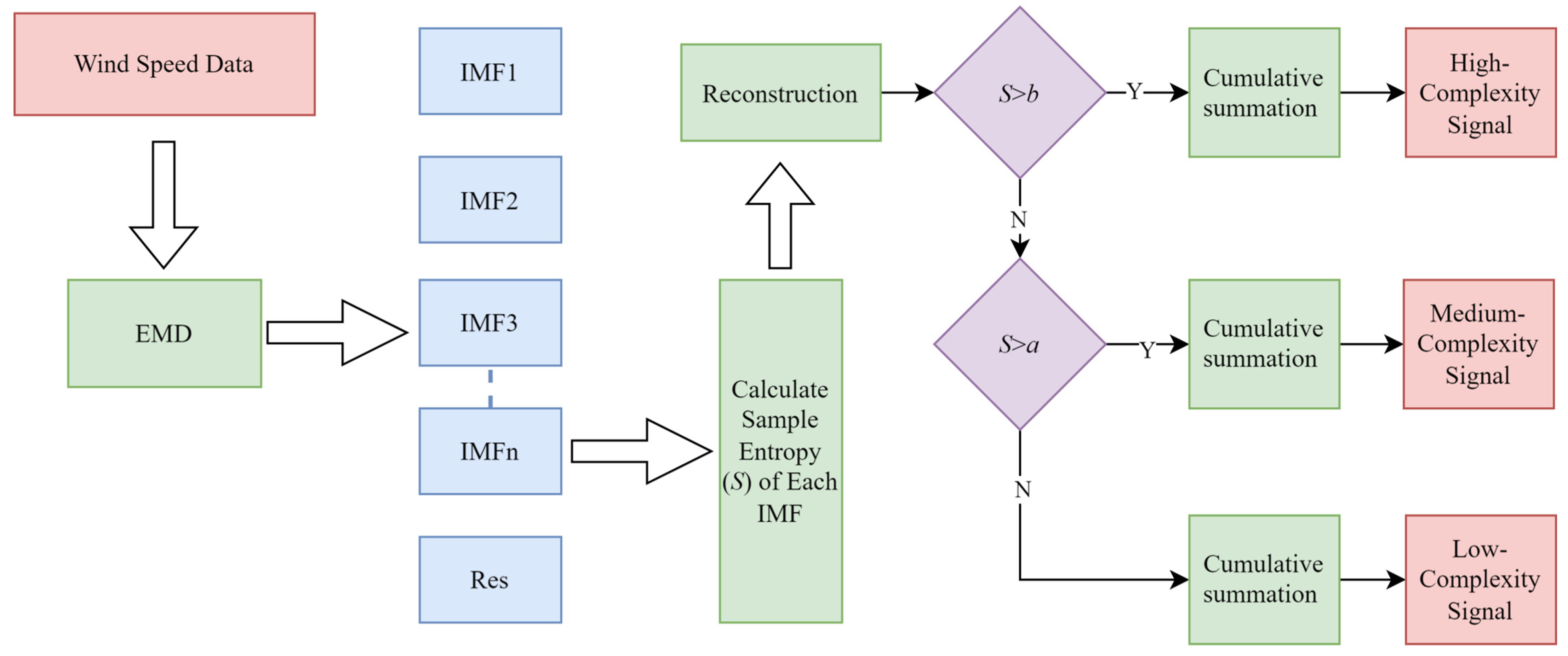
Based on the magnitude of sample entropy, the complexity of the decomposed components of wind speed can be assessed. A higher sample entropy indicates greater complexity in the wind speed sequence, indicating that the wind speed data fluctuate more violently. Conversely, as sample entropy decreases, the wind speed sequence becomes more orderly or periodic. By calculating the sample entropy of the individual decomposed elements and considering the magnitude of these values, the components are reconstructed into three categories: high-complexity, medium-complexity, and low-complexity signals, which serve as the three feature inputs for the model. Subsequences exhibiting sample entropy values greater than some up limit value b are superimposed to form the high-complexity component, those with sample entropy values less than some down limit value a are superimposed to form the low-frequency component, and those with sample entropy values between a and b are superimposed to form the medium-complexity component. This method merges multiple components into three inherent components to simplify the structure of the model input, reducing the computational complexity during prediction, with the detailed procedure illustrated in Figure 3.

3.3. Rolling Decomposition Mechanism-Based Combined LSTM Model for Wind Speed Forecasting

Considering the randomness and volatility inherent in wind speed data, this study aims to construct an LSTM-based combined wind speed prediction model by reconstructing decomposition components using the sample entropy method based on the rolling decomposition approach. Due to the possibility of outliers caused by sensor malfunctions or external environmental interference in the wind speed data, the input wind speed data undergo preprocessing first to mitigate the negative impact on prediction accuracy. This preprocessing includes detecting and addressing anomalies and gaps in the dataset. For the preprocessed data, a rolling decomposition–merging–prediction method is then used for refined forecasting. The complete procedure is outlined in the following steps, with the specific procedure shown in Figure 4.
Step 1: Initialization and Rolling Data Partitioning
In light of the properties of the dataset and the prediction requirements, an appropriate data window size is determined. This window captures the local features of the temporal data. The known temporal data are split into multiple sets through a rolling process, with each set having the window size as input and the next data point as the output. Typically, a portion of 80% of the dataset is dedicated to training the model, and the remaining 20% is held for testing.
Step 2: Decomposition and Merging
For the input part of each dataset, the EMD technique is used to break the signal down into multiple IMFs. The IMFs are then merged into three components with high, medium, and low complexity contents, based on the calculated sample entropy value of each component in the signal.
Step 3: Model Construction and Training
The merged signals serve as the model’s input to forecast the next data point, with the model’s output being the undecomposed output part of each dataset. The model is optimized with the training set data.
Step 4: Wind Speed Prediction
For the test dataset, the EMD and signal merging process from Step 2 is first repeated. The merged signals are then fed into the trained model to make predictions and retrieve the forecast for the next data point. The same operation is repeated for the next set of data in the test set. After each prediction, the new known data point is added to the window, and the model input is updated until all data points in the test set have been predicted.
Step 5: Calculation of Prediction Results
The divergence between the predicted outcomes and the actual values is measured. The model’s prediction performance is assessed based on error metrics, evaluating the model’s accuracy and reliability.

4. Case Study and Analysis

4.1. Data Source

In this experiment, three different datasets collected from a wind farm—labeled Dataset A, B, and C—were used. Each dataset consists of 2000 data points, with a sampling interval of 1 s. Table 1 presents the statistical properties of the three datasets. The experimental data undergo initial preprocessing before being divided into subsets for training and evaluation.
From the table above, it can be seen that the maximum wind speeds for datasets A, B, and C all exceed 12 m/s, indicating relatively strong wind conditions. Dataset B shows the higher minimum wind speed, while datasets A and C have lower minimum wind speeds. Dataset B has the highest average wind speed, at 9.69 m/s, indicating that the overall wind strength is slightly greater than that of the other two datasets. In terms of wind speed fluctuations, datasets A and C have higher standard deviations, implying greater variability in wind speeds, while dataset B has the lowest standard deviation, indicating the most stable wind speed changes.

4.2. Performance Evaluation

To assess the predictive accuracy of the model on wind speed time series, three commonly used statistical metrics have been selected for assessment. The following are the three evaluation metrics employed, with their respective definitions:
(1)
Mean Absolute Error (MAE)
The MAE represents the mean of the absolute errors between the predicted and actual values, serving as a measure of the average deviation in absolute terms. A lower MAE value signifies a smaller gap between the model’s predictions and the actual values, reflecting higher prediction accuracy. The formula is as in (4).
M A E = 1 m i = 1 m x i y i
where x i denotes the actual measurement, y i denotes the forecasted value, and m refers to the entire dataset’s point count.
(2)
Root Mean Squared Error (RMSE)
The RMSE represents the square root of the mean of the squared differences between the forecasted and actual values. A lower RMSE indicates a smaller gap between the forecasted and observed results, which reflects better prediction accuracy. The formula is as in (5).
R M S E = 1 m i = 1 m x i y i 2
where x i denotes the actual measurement, y i denotes the forecasted value, and m refers to the entire dataset’s point count.
(3)
Mean Absolute Percentage Error (MAPE)
MAPE quantifies the difference between the forecasted and actual values, expressed as a percentage. It reflects the gap between the forecasted and observed values, serving as a common metric to assess prediction accuracy and evaluate model performance. The formula is as in (6).
M A P E = i = 1 m x i - y i y i × 100 % m
where x i denotes the actual measurement, y i denotes the forecasted value, and m refers to the entire dataset’s point count.

4.3. Experimental Results and Data Leakage Analysis

(1) Experimental Results
In this experiment, the parameters for the EMD-LSTM model are set as follows: the Adam optimizer is used with a maximum of 50 iterations, an initial learning rate of 0.004, a learning rate decay factor of 0.5 every 20 iterations, and a minimum batch size of 64. The sample entropy parameters are set to m = 2 and r = 0.2, with a component merging threshold of (0.1, 0.6). It should be noted here that all parameters employed here are set based on trial and error, without any formal tuning. The model development, training, and validation are conducted on a desktop system configured with an Intel (R) i7-10700k CPU, 16 GB of memory, and run in the Matlab 2024b software environment.
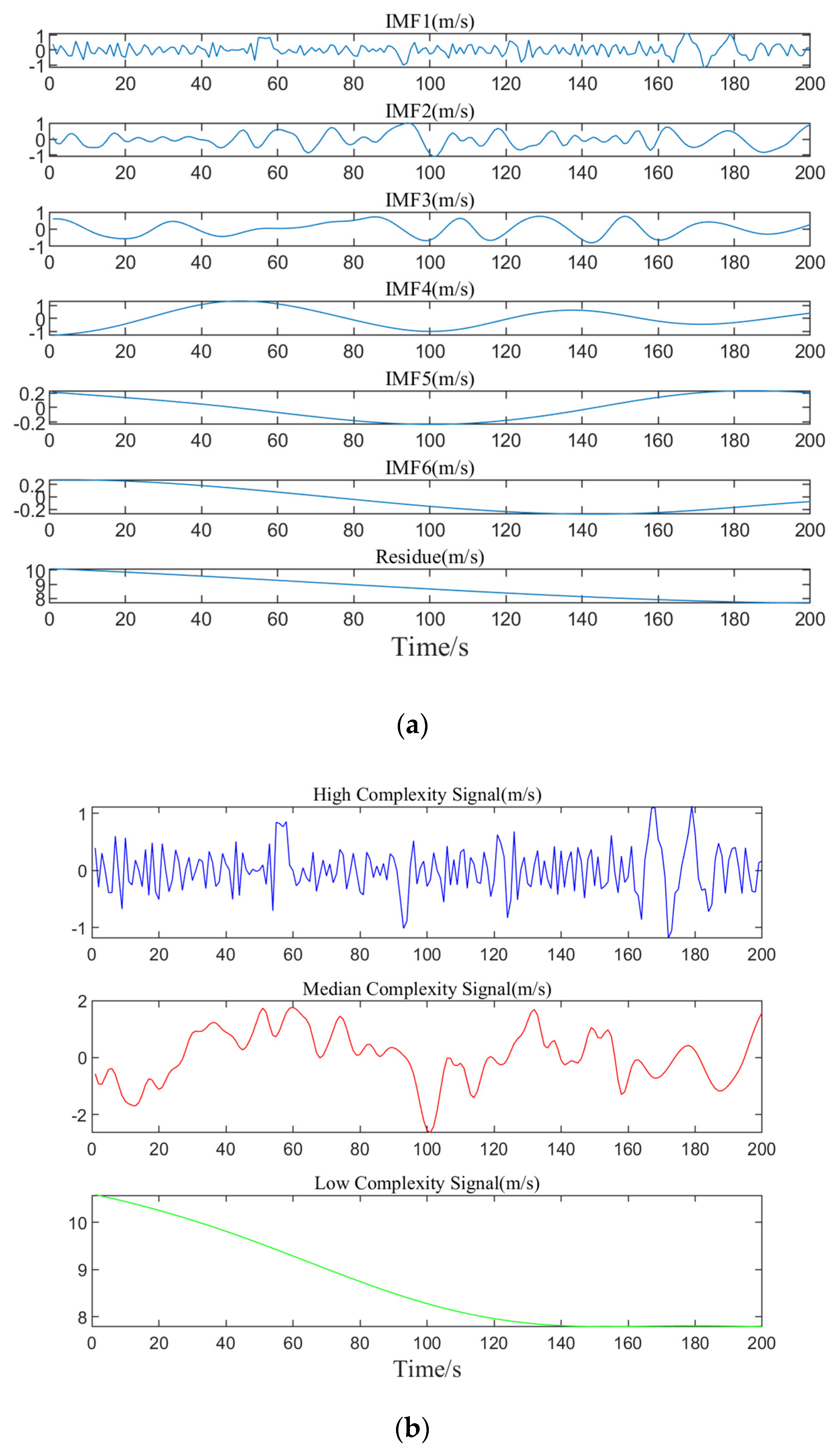
Following the steps for the EMD method, the preprocessed dataset A is rolled and divided for decomposition, transforming the non-stationary wind speed data into multiple IMFs along with a residual component. Due to the large number of data groups resulting from the division, it is not feasible to display and analyze all of them. Therefore, this result only presents the decomposition and merging of one set of data, as shown in Figure 5.
From Figure 5a, it can be seen that through the EMD method, the data are progressively broken down into multiple IMFs and a residual term, revealing the multi-level variation characteristics of the data from high complexity to low complexity, to some extent, from high frequency to low frequency. As the decomposition proceeds, the frequency of the subsequent IMF components gradually decreases, the volatility weakens, and eventually tends to be stable, demonstrating the change process of the data ranging from high to low frequencies. Figure 5b shows that the merged components are categorized into high, medium, and low-frequency ranges, each showing different fluctuation trends. By analyzing these three frequency components, the model’s feature input is simplified, which more accurately captures the signal’s change trend in the prediction model, thus enhancing the model’s predictive accuracy.
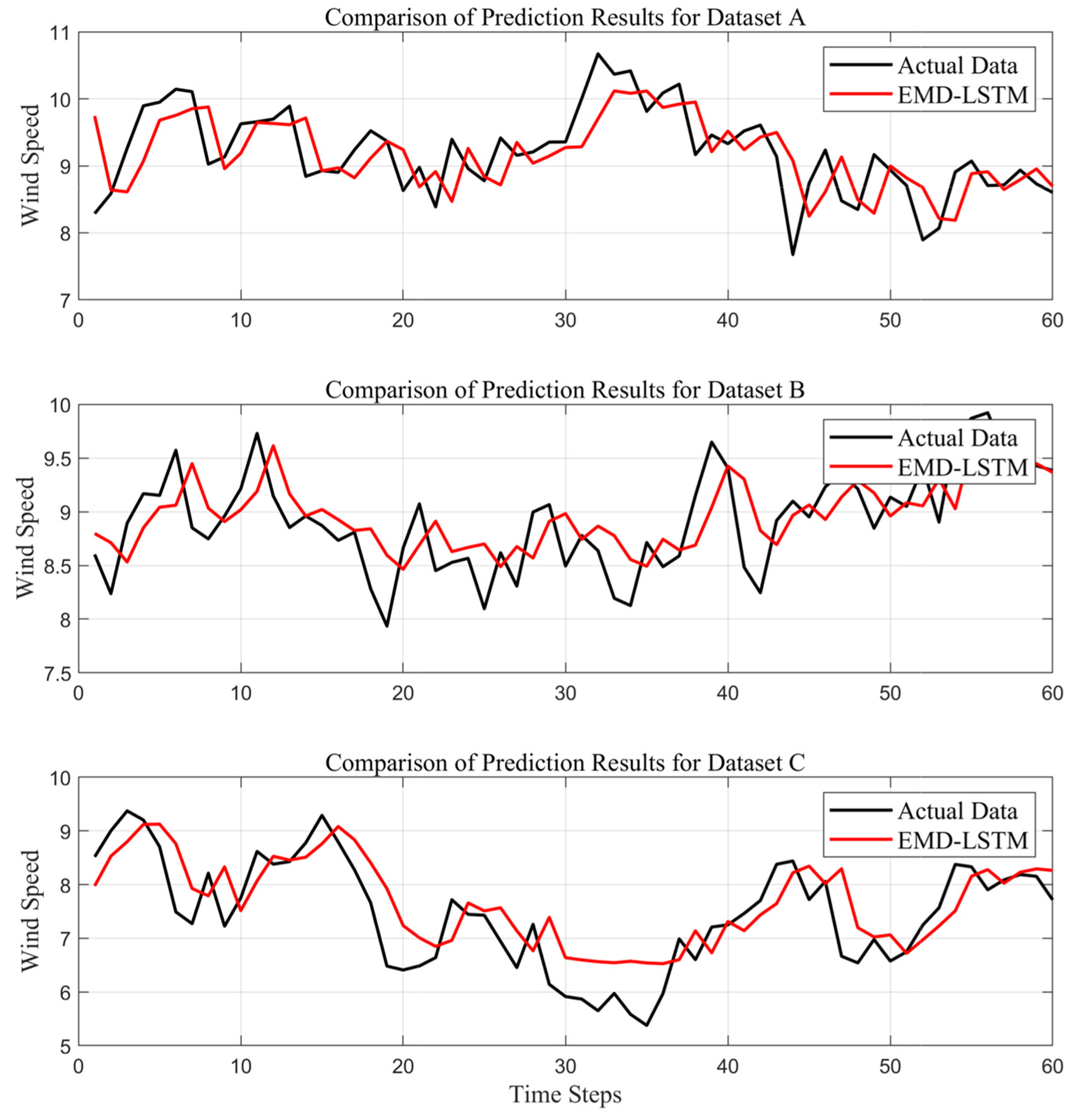
To assess the forecasting performance of the EMD-LSTM model across different datasets, single-step wind speed prediction experiments were conducted using datasets A, B, and C. According to the rolling decomposition–synthesis–forecasting steps, the data rolling window size is set to 200 (i.e., using 200 historical samples of wind speed to predict the next data point), and the data are divided into 1800 groups, using the first 1740 data samples for training and the final 60 samples for testing. The experiments are conducted under the same model parameters, and the forecasting outcomes of the test sets for different groups of data are plotted as shown in Figure 6.
Comparing the trend in wind speed prediction results for different datasets, all prediction curves have essentially captured the variation trend of the actual values. However, it is evident that the prediction results for dataset B are the best, with the model effectively capturing the rising and falling fluctuation trends in the data.
To more quantitatively evaluate the model’s predictive performance, the model’s strengths and weaknesses are evaluated by analyzing its performance across different experimental datasets using a range of evaluation metrics. The evaluation metrics for each model, including MAPE, MAE, and RMSE, are listed in Table 2. These metrics can help explain the model’s predictive accuracy, thereby better selecting a model suitable for wind speed prediction.
Based on the defined evaluation metrics, a comparative analysis of the prediction model performance for datasets A, B, and C is conducted. The analysis reveals that dataset B yields the best performance, achieving 0.2921 m/s for MAE, 3.3151% for MAPE, and 0.3566 m/s for RMSE. The difference between its forecasts and the true value is minimized, and its accuracy is the highest. The prediction performance of dataset A is also relatively good, with all metrics slightly higher than those of dataset B. However, dataset C has the worst prediction performance. The MAE, MAPE, and RMSE values for this dataset stand at 0.5165 m/s, 7.3877%, and 0.6320 m/s, showing a notable increase compared to the other two datasets. This may reflect the higher complexity inherent in dataset C. Overall, for these three datasets, the prediction errors are relatively small, suggesting that the model demonstrates strong stability.
(2) Prediction Error Analysis
To further analyze the prediction errors of the proposed EMD-LSTM, the key statistical metrics, i.e., maximum, minimum, mean, median, and standard deviation, are calculated. The results for the different datasets are shown in Table 3.
As shown in Table 3, in terms of maximum and minimum errors, Dataset A has a maximum error of 0.9684 m/s and a minimum error of −1.4543 m/s, while Dataset C has a maximum error of 0.8648 m/s and a minimum error of −1.6303 m/s. Compared to Dataset B, which has a maximum error of 0.6922 m/s and a minimum error of −0.8200 m/s, both Datasets A and C exhibit larger negative error extremes. This indicates that, across the three datasets, the model’s predictions for Datasets A and C are slightly lower than the true values at certain time points. This discrepancy may stem from anomalous fluctuations in wind speed data, which the model struggles to capture accurately.
Regarding mean errors, Dataset A has a mean error of 0.0452 m/s, slightly above zero, suggesting that predictions are marginally higher than true values on average. Dataset B has a mean error of −0.0481 m/s, slightly below zero, indicating that predictions are marginally lower than true values. Dataset C, however, shows a larger negative mean error of −0.2125 m/s, reflecting a consistent underprediction by the model.
In terms of standard errors, Dataset A has a standard error of 0.5172 m/s, Dataset B 0.3564 m/s, and Dataset C 0.6003 m/s. Dataset B’s smaller standard error indicates a more concentrated error distribution and better model stability. In contrast, the larger standard errors of Datasets A and C suggest higher error dispersion and poorer prediction stability. This is likely attributable to the more complex and variable wind speed patterns in Datasets A and C, making it challenging for the model to achieve accurate fitting and resulting in increased error variability.
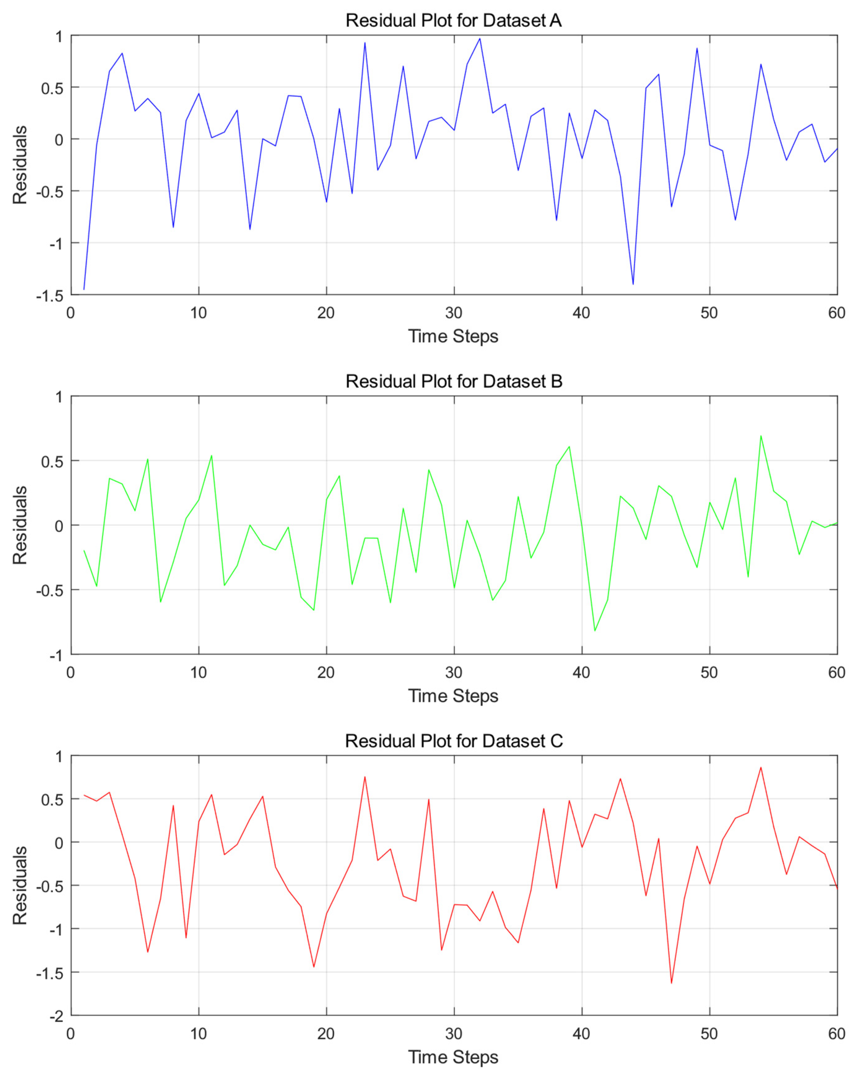
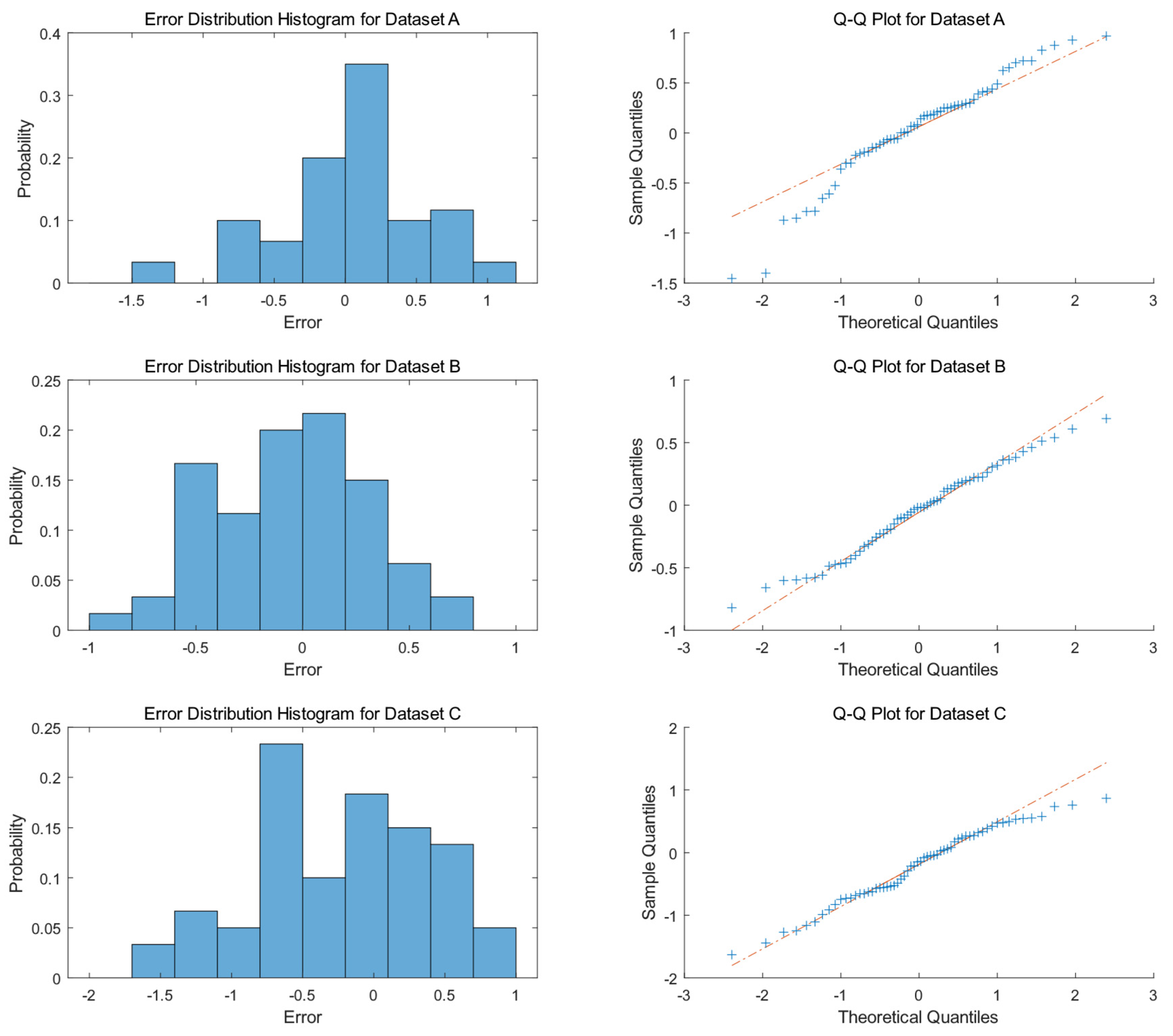
Additionally, the errors are visualized through residual plots illustrated in Figure 7 and error distribution histograms and Q-Q plots illustrated in Figure 8 to further investigate the underlying causes of the model’s prediction errors.
Figure 7 clearly shows that the residuals of Dataset A exhibit frequent and significant fluctuations, ranging between −1.5 and 1, with multiple peaks and troughs. This indicates substantial deviations between the model’s predictions and actual values at these time steps. Moreover, the residuals lack a discernible pattern, showing no clear periodic fluctuations or consistent trend lines, and are randomly distributed around zero. In contrast, the residuals of Dataset B demonstrate relatively milder fluctuations, generally within the range of −1 to 1. While appearing random, their distribution around zero is uneven, with varying degrees of deviation across different intervals. Dataset C exhibits even wider residual fluctuations, with some time steps approaching −2, highlighting more pronounced deviations between predicted and actual values. The residuals show no apparent pattern and are chaotically distributed across the axis. Overall, the residuals of all three datasets deviate from the ideal state of random distribution. This phenomenon is closely tied to the stochastic and complex nature of wind speed sequences. The inherent uncertainty and complexity of wind speed make it challenging for the model to accurately capture its variations, resulting in residuals that fail to conform to an ideal random distribution.
The histogram illustrated in Figure 8 reveals that the prediction errors of Dataset A are predominantly concentrated between −1 and 1, with a peak near 0, exhibiting a probability of approximately 35%. A minor distribution is observed around −1.5, though with a probability of less than 5%. Thus, the error distribution of Dataset A is basically symmetric, with limited instances of under-prediction. Dataset B demonstrates a relatively symmetric error distribution, with errors uniformly distributed between −1 and 1, showing more balanced probabilities across error intervals compared to Dataset A. Dataset C exhibits a more dispersed error distribution, with higher probabilities for errors between −1 and 0.5, peaking near −0.5. Errors around −2 and 1 also occur, but with lower probabilities. Compared to Datasets A and B, Dataset C shows a higher probability of errors in the negative region, indicating a greater tendency for the model to under-predict on this dataset.
The right column of Figure 8 illustrates the Q-Q plots, which further validate the normality of residuals across different datasets. For Dataset A, the data points do not strictly align with the theoretical line on the Q-Q plot, particularly deviating at the tails, especially on the left side, indicating that its residual distribution differs from a normal distribution and does not satisfy the normality assumption. Dataset B’s data points closely cluster around the theoretical line, suggesting that the sample quantiles closely match the theoretical quantiles, implying that its residual distribution is relatively similar to a normal distribution. In Dataset C’s Q-Q plot, the data points exhibit significant deviations from the theoretical line, particularly in the middle section, indicating a substantial divergence of its residual distribution from the theoretical normal distribution model.
In summary, the error distributions of the EMD-LSTM model vary across different datasets. Dataset B’s error distribution is closest to a normal distribution, indicating relatively better predictive performance of the model. In contrast, the error distributions of Datasets A and C exhibit varying degrees of deviation from normality.
(3) Data Leakage Analysis
From a methodological perspective, the traditional EMD approach carries the risk of information leakage. The conventional method involves performing EMD on the entire dataset to obtain all IMF components before dividing the data into training and test sets. Since the IMF components are derived from the overall trend of the original wind speed sequence, the training set inadvertently gains knowledge of the test set’s fluctuation trends during model training. This leads to artificially inflated prediction accuracy on the test set, failing to reflect the model’s true predictive capability.
In contrast, the rolling EMD method proposed in this study effectively addresses this issue at its core. The method begins by dividing the data into multiple input–output pairs based on a specific rolling window size. Subsequently, the input data undergo decomposition and reconstruction as described in the paper, yielding three feature-rich components that correspond one-to-one with the output. These input–output pairs are then divided into training, validation, and test sets, followed by model training and prediction. During the training phase, the inputs consist of the three decomposed components derived solely from historical records within the rolling window, ensuring that only past wind speed information is utilized. The output during training is the data for the next time step, which are pre-divided and do not participate in the decomposition process. This ensures that the model does not gain access to any future information during training, fundamentally preventing information leakage. During the prediction phase, once the model is trained and begins predicting on the test set, the test set data remain entirely independent of the training process. The model can only rely on the knowledge acquired during training to make predictions, free from interference by other data sources. This approach guarantees the authenticity and reliability of the prediction results.
(4) Potential for Practical Applications
In practical wind speed prediction scenarios, the trained EMD-LSTM model may run through a systematic process to predict wind speeds at each time step. Specifically, for predicting the wind speed at time step T, the model first retrieves historical wind speed data within a predefined rolling window prior to time T. These data are then subjected to Empirical Mode Decomposition (EMD), which breaks them down into multiple Intrinsic Mode Functions (IMFs). These IMFs are subsequently reconstructed into three distinct frequency-specific components using the sample entropy method. The LSTM network leverages these three components to perform a detailed prediction analysis, ultimately generating the predicted wind speed value for time T. Once this prediction is completed, the model shifts its focus to predicting the wind speed for the next time step, T + 1. At this stage, the model integrates the actual wind speed data newly updated at time T into the rolling window. To maintain a consistent window size, the oldest data point is removed, ensuring computational stability and consistency throughout the process. Following the data update, the model reapplies EMD to decompose the newly updated rolling window data and reconstructs them using the sample entropy method. The LSTM network then utilizes these newly generated components to predict the wind speed for time T + 1. This continuous rolling prediction mechanism ensures that the output data do not participate in the decomposition process, thereby eliminating any risk of information leakage. This approach guarantees the authenticity and reliability of the prediction results, making the EMD-LSTM model a robust tool for practical wind speed prediction applications.

4.4. Parameter Analysis

(1) Sample Entropy Parameters
To investigate the effects of different combinations of sample entropy parameters m and r on the prediction performance of the EMD-LSTM model, a sensitivity analysis is performed. In this experiment, the key parameters of sample entropy are systematically defined and varied, with m taking values of [1, 2, 3] and r taking values of [0.1, 0.15, 0.2, 0.25]. These parameter combinations are comprehensively tested across three different datasets to provide an in-depth analysis of how variations in sample entropy parameters affect the prediction results of the EMD-LSTM model. The prediction results of EMD-LSTM with different sample entropy parameter combinations are presented in Table 4, Table 5 and Table 6 for various datasets.
From Table 4, for Dataset A, when m = 1, as r increases, the MAE, RMSE, and MAPE first increase and then decrease, with small fluctuations. When m = 2, the changes in the indicators are more complex, with the RMSE reaching a relatively low value when r = 0.2. For m = 3, the indicators show a relatively slow overall change, but the values are higher. It can be observed that in Dataset A, different parameter combinations affect model performance, with the combination of m = 2 and r = 0.2 performing best according to the indicators.
From Table 5, for Dataset B, when m = 1, the differences in the indicators for different parameter combinations are significant, especially when r = 0.15, where all error metrics are noticeably high. When m = 2, the indicators remain relatively stable as r changes, and the overall values are lower. For m = 3, there is some fluctuation in the indicators. This suggests that in Dataset B, the parameter setting of m = 2 leads to a more stable model performance, with the combination of m = 2 and r = 0.2 yielding the lowest error metrics and the best prediction performance.
From Table 6, for Dataset C, when m = 1, the error indicators fluctuate significantly as r changes. For m = 2, when r = 0.15, both MAE and RMSE are relatively small, while MAPE remains within a reasonable range when r = 0.2. For m = 3, the indicators exhibit a wider range of variation. Overall, for Dataset C, the model performs best with m = 2, showing good adaptability to different values of r, with the combination of m = 2 and r = 0.2 achieving a good balance across the evaluation metrics.
Based on the analysis of these three datasets, selecting the sample entropy parameters m = 2 and r = 0.2 consistently leads to the best and most balanced results across all evaluation metrics.
(2) Component Reconstruction Threshold Parameters
With the sample entropy parameters fixed at m = 2 and r = 0.2, a sensitivity analysis is conducted to explore the impact of different component merging threshold parameter combinations on the prediction performance of the EMD-LSTM model. In the experiment, a series of threshold combinations are defined, specifically [mid-frequency and low-frequency threshold a, mid-frequency and high-frequency threshold b], with the following values: [0.05, 0.5]; [0.1, 0.6]; [0.15, 0.7]; [0.2, 0.8]. These key parameters are systematically varied, and the model’s prediction performance is comprehensively tested. The prediction results of this experiment with various threshold parameter combinations for different datasets are presented in Table 7, Table 8 and Table 9.
From the model prediction results for Datasets A, B, and C as seen in Table 7, Table 8 and Table 9, respectively, it is evident that different threshold parameter combinations have varying impacts on the evaluation metrics. In Dataset A, the fluctuations in the indicators are relatively small as the parameters change, with a = 0.15 and b = 0.70 yielding the best performance in RMSE. In Dataset B, when a = 0.1 and b = 0.6, all three-evaluation metrics reach their lowest values, indicating outstanding prediction accuracy. In Dataset C, the indicator fluctuations are more stable, with a = 0.2 and b = 0.8 yielding a relatively low MAPE.
Overall, although the parameter combination a = 0.1 and b = 0.6 does not achieve the lowest values for all metrics in every dataset, it performs well across the board in terms of overall prediction accuracy, particularly excelling in Dataset B. Therefore, the combination of a = 0.1 and b = 0.6 is selected as the threshold for component merging.

4.5. Comparisons with Other Methods

To comprehensively validate the performance of the proposed model, comparative experiments are conducted between the EMD-LSTM model and other wind speed prediction methods, including SVM, ARIMA, GRU, and LSTM, across the three datasets. All experiments are carried out under the same experimental conditions, using the same datasets and evaluation metrics to ensure consistency.
Experimental Setup: The experiments are conducted on a desktop computing platform with an Intel(R) i7-10700K CPU, 16 GB of RAM, and Matlab 2024b software environment, where the model construction, training, and validation are systematically carried out.
Model Parameter Settings: For the ARIMA model, the parameters are set as (p, d, q) = (3, 1, 2). The SVM model utilizes a Gaussian kernel with automatic scale adjustment. The GRU and LSTM models have identical parameters: the Adam algorithm as the optimizer, a maximum of 50 iterations, an initial learning rate of 0.004, a learning rate decay factor of 0.5 every 20 iterations, and a minimum batch size of 64. The EMD-LSTM model uses sample entropy parameters m = 2, r = 0.2, and component merging thresholds of (0.1, 0.6).
(1) Prediction Accuracy
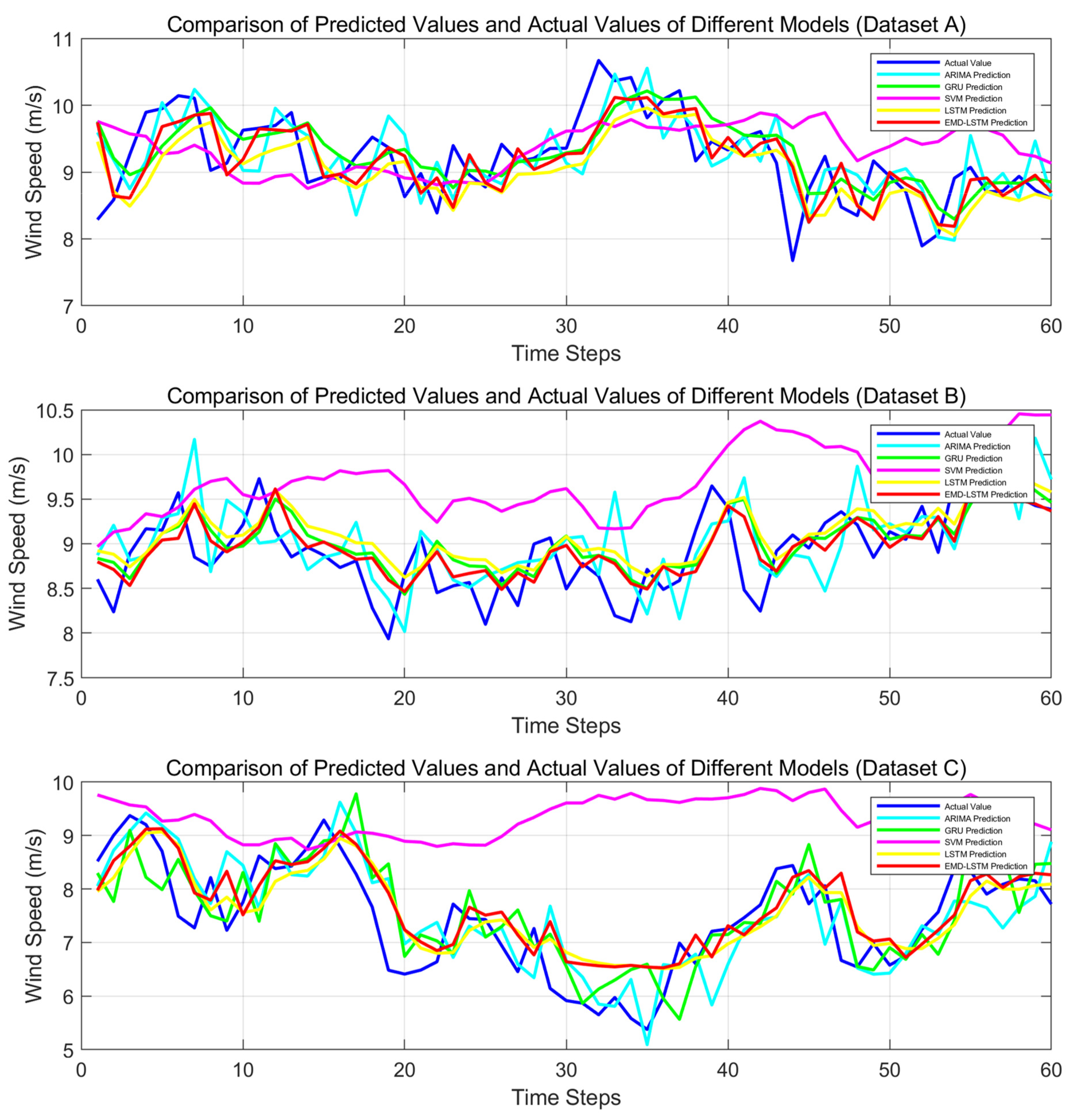
The prediction curves for different method combinations are plotted as shown in Figure 9. It can be clearly observed from this figure that in Dataset A, the prediction curves of all models fluctuate frequently, with the EMD-LSTM model’s curve being relatively closer to the actual value curve, effectively capturing the wind speed variation trend. In Dataset B, the models show varied performance, with some models exhibiting significant deviations in their prediction curves. However, the EMD-LSTM model has a smaller deviation from the actual values at most time steps, and its fluctuations closely mirror the variations in actual wind speed. In Dataset C, in the face of complex wind speed changes, the EMD-LSTM model’s prediction curve follows the actual values more closely than the other models, showing a higher degree of alignment at key wind speed change points.
Overall, across all three datasets, while each model reflects wind speed changes to some extent, the EMD-LSTM model demonstrates superior performance with a higher degree of alignment between its prediction curve and the actual value curve, as well as better consistency in fluctuation trends. This indicates its stronger ability to capture wind speed variation characteristics and its higher prediction accuracy, outperforming the other comparison models.
By analyzing the model’s performance across different datasets using a variety of evaluation criteria, the superiority or inferiority of the models can be assessed. The evaluation metrics, including MAE, MAPE, and RMSE, are listed in Table 10, Table 11 and Table 12, respectively, for various models on different datasets.
From the above Table 10, Table 11 and Table 12, it can be observed that in Dataset A, compared to the LSTM model, the EMD-LSTM model achieves a reduction of approximately 11.46% in MAE and 7.97% in RMSE. While MAPE remains the same, the former two metrics demonstrate superior performance. When compared to other models, the ARIMA and SVM models have significantly higher error metrics than EMD-LSTM, while the GRU model shows some similarity in certain indicators, but overall, EMD-LSTM controls errors more effectively. In Dataset B, the EMD-LSTM model reduces MAE by approximately 14.44%, RMSE by 13.89%, and MAPE by 15.07% compared to the LSTM model, showing a significant improvement in prediction accuracy. In comparison to other models, SVM exhibits much higher error metrics than EMD-LSTM. ARIMA and GRU models are competitive but still lag behind the EMD-LSTM model. In Dataset C, the EMD-LSTM model reduces MAE by approximately 5.40%, RMSE by 2.56%, and MAPE by 3.92% compared to the LSTM model, achieving better prediction accuracy. Compared to other models, SVM has the largest error, and both ARIMA and GRU models have higher error metrics than EMD-LSTM.
Considering the evaluation across all three datasets, the EMD-LSTM model shows a significant reduction in MAE, RMSE, and MAPE compared to the other models, especially the LSTM model, indicating superior prediction performance.
(2) Model Complexity Analysis
In addition to focusing on prediction accuracy, computational complexity is also a critical consideration, as it directly affects the efficiency and feasibility of the model in practical applications. Here, the time spent in the prediction stage of various models in the same computer environment is used as the alternative indicator to represent computational complexity. The time consumption of ARIMA, GRU, SVM, LSTM, and the proposed EMD-LSTM during the prediction phase is shown in Table 13.
From the perspective of time consumption during the prediction phase shown in Table 13, the computational complexity of different models shows little variation across datasets. The SVM model has the shortest prediction time on Datasets A, B, and C, indicating higher computational efficiency and relatively lower complexity during the prediction phase. The GRU model also has a shorter prediction time, placing its computational complexity at a relatively low level. The time consumption of the LSTM and EMD-LSTM models is similar, with both models exhibiting comparable computational complexity across the three datasets. In contrast, the ARIMA model shows significantly higher prediction time on all three datasets compared to the other models. EMD-LSTM, as a newly proposed method, has a prediction stage time consumption of approximately 0.36 s across these three datasets, which is comparable to GRU and LSTM, slightly higher than SVM (approximately 0.12–0.21 s), but significantly lower than ARIMA (approximately 1.2–1.3 s). This indicates that EMD-LSTM outperforms ARIMA in efficiency and approaches GRU and LSTM, but is slightly inferior to SVM. The advantage of EMD-LSTM likely lies in its combination of EMD (Empirical Mode Decomposition) and LSTM, enabling it to better capture multi-scale features in complex time series, making it suitable for nonlinear and non-stationary data prediction tasks. Although its computational time is slightly longer than that of GRU and LSTM, it remains suitable for practical applications and shows greater potential in accuracy and feature extraction capabilities.

4.6. Statistical Analysis and Nonparametric Test

(1) Statistical Analysis
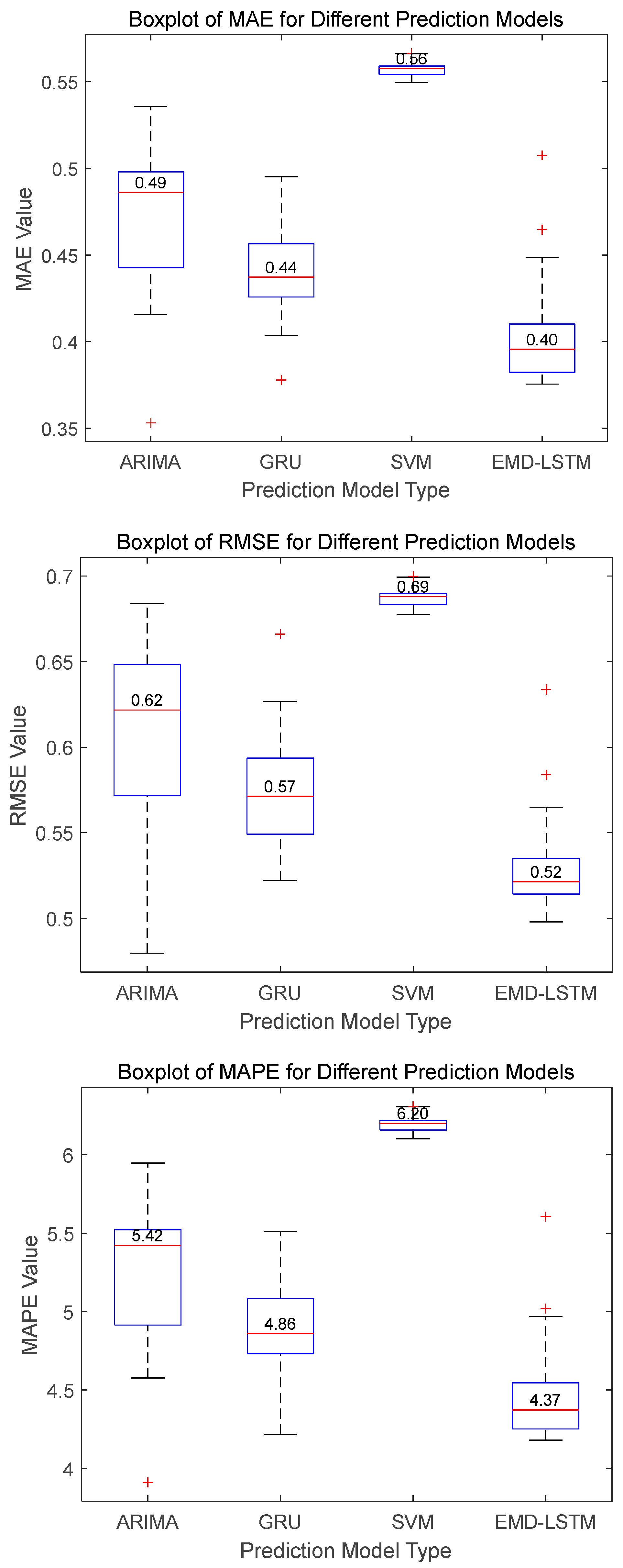
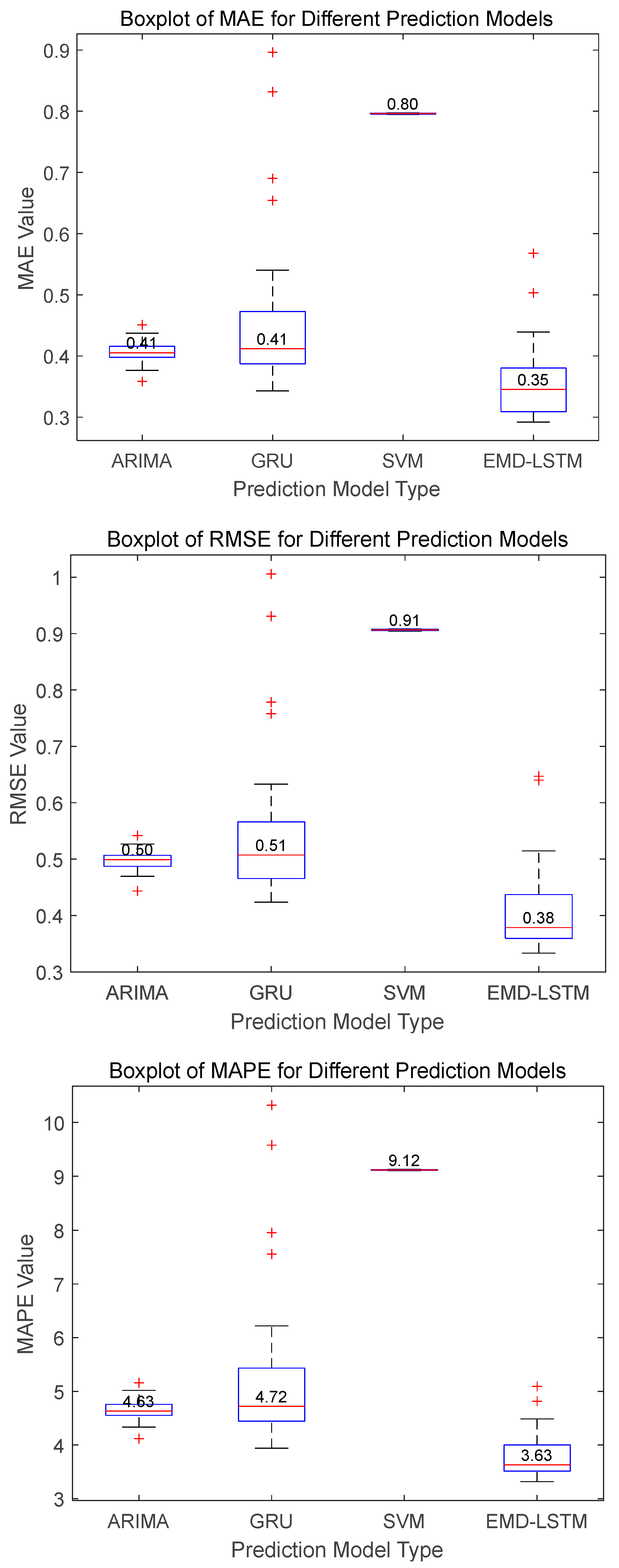
To comprehensively and accurately assess the performance of the proposed EMD-LSTM method compared to other existing models such as ARIMA, SVM, and GRU in wind speed prediction, each of the aforementioned models is run 30 times separately under the same experimental environment and parameter settings. The evaluation metrics of different models are statistically analyzed. Through multiple independent runs and systematic statistical analysis, the performance of each model on different datasets is obtained, and a solid data foundation is provided for comparing their advantages and disadvantages. For Dataset A, the MAE, RMSE, and MAPE values of ARIMA, SVM, GRU, and EMD-LSTM models in 30 runs are obtained; their boxplots are illustrated in Figure 10. The statistical comparisons of the three metrics for different algorithms on Dataset B and Dataset C are presented in Figure 11 and Figure 12, respectively.
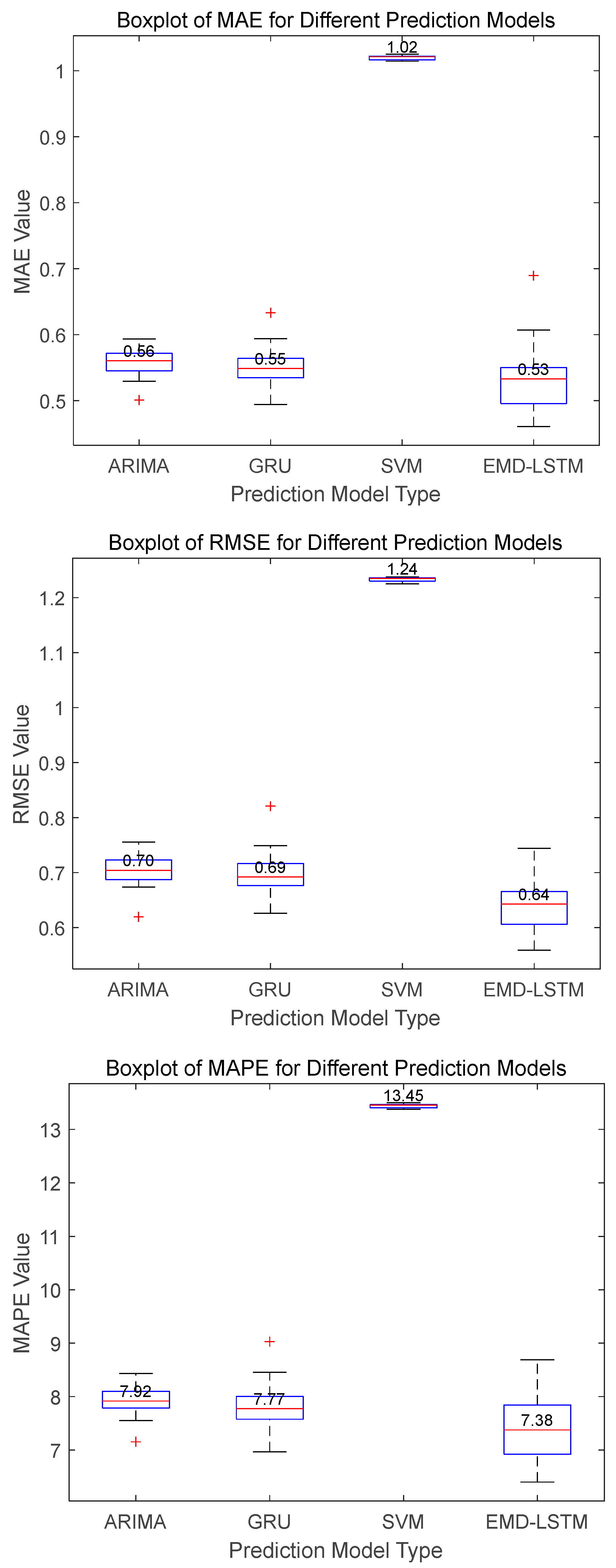
For Dataset A, the boxplots in Figure 10 illustrate that the EMD-LSTM model achieves median values of MAE, RMSE, and MAPE at 0.40, 0.52, and 4.37%, respectively, over 30 runs. These figures represent improvements of approximately 9.09%, 8.77%, and 10.08% over the best values obtained by other considered methods, which are 0.44, 0.57, and 4.86%. Furthermore, the EMD-LSTM exhibits a slightly narrower box width compared to ARIMA and GRU, indicating higher stability relative to these methods, while SVM, despite its higher stability, shows significantly higher median values, suggesting lower accuracy than EMD-LSTM. For Dataset B, statistical results shown in Figure 11 reveal that EMD-LSTM attains median values of MAE, RMSE, and MAPE at 0.35, 0.38, and 3.63%, respectively, over 30 independent runs, marking improvements of 14.63%, 24%, and 21.59% over the best values from other comparative algorithms, which were 0.41, 0.51, and 4.63%. For Dataset C illustrated in Figure 12, EMD-LSTM achieves median values of MAE, RMSE, and MAPE at 0.53, 0.64, and 7.38%, respectively, over 30 independent runs, outperforming the best values from other comparative algorithms by 3.64%, 7.25%, and 5.02%, which are 0.55, 0.69, and 7.77%. In summary, based on the median values of multiple experimental metrics, the EMD-LSTM method demonstrates improvements of at least 3.64%, 7.25%, and 5.02% over other methods across the considered test datasets.
(2) Nonparametric Test
To further validate the effectiveness of the proposed EMD-LSTM model compared to the other three models, a non-parametric test analysis is conducted. The Wilcoxon test is applied, with the significance level 0.05 as the criterion. The null hypothesis assumes no significant difference between EMD-LSTM and the other models (h = 0), while the alternative hypothesis assumes a significant difference (h = 1). Pairwise comparisons of the EMD-LSTM model with ARIMA, GRU, and SVM are made across the three datasets, using the specified significance level as the threshold. The results of the non-parametric tests for the three datasets are presented in Table 14, Table 15 and Table 16.
The Wilcoxon test results as shown in Table 14, Table 15 and Table 16 for MAE, MAPE, and RMSE across the three datasets show that the p-values for all models compared to EMD-LSTM are significantly less than 0.05, with h = 1 in all cases. This indicates that, across all datasets and evaluation metrics, there are significant differences in prediction performance between the ARIMA, GRU, SVM models, and the EMD-LSTM model. As previously discussed from the boxplots in Figure 10, Figure 11 and Figure 12, the EMD-LSTM model exhibits lower median values for MAE, RMSE, and MAPE, indicating superior prediction accuracy. These Wilcoxon test results further confirm, from a statistical perspective, that the EMD-LSTM model has a significant advantage over ARIMA, GRU, and SVM models in prediction performance, thereby validating the model’s effectiveness.
5. Conclusions

A combined EMD-LSTM forecasting model, utilizing a rolling decomposition–merging–forecasting approach and sample entropy reconstruction technology is introduced to improve the accuracy of wind speed forecasting. Based on the experimental case analysis, the conclusions are as follows:
(1) The use of rolling decomposition ensures unknown data will not be leaked in advance, avoiding the issue of overestimating prediction accuracy due to the involvement of future information in model training. This proposed EMD-LSTM model provides a realistic and reliable assessment of prediction accuracy.
(2) Employing sample entropy reconstruction, the decomposed IMFs and residual signals are subsequently aggregated into three distinct frequency-fluctuating signals, which are sent as input features to the LSTM for prediction. This process not only mitigates the inherent fluctuations within the data but also unveils its underlying intrinsic structure. Consequently, the model is better equipped to capture the underlying trends in wind speed variations, thereby enhancing the accuracy of the predictions.
(3) The statistical experimental results demonstrate that the proposed EMD-LSTM model achieves improvements in MAE, RMSE, and MAPE metrics by at least 3.64%, 7.25%, and 5.02%, respectively, compared to other methods across the three evaluated test datasets from a real-world wind farm. Furthermore, the Wilcoxon test results provide robust statistical evidence, confirming that the EMD-LSTM model significantly outperforms ARIMA, GRU, and SVM models in prediction performance.
Therefore, it can be concluded that the proposed hybrid EMD-LSTM model demonstrates competitive performance when validated on data from three distinct wind generators at an actual wind farm. The model consistently outperforms existing GRU, ARIMA, and LSTM models in terms of statistical metrics, while also effectively mitigating the risk of information leakage. However, the decomposition process applied to the input data of each sample pair introduces additional computational overhead, leading to increased time consumption during the training phase. Despite this limitation, the proposed approach remains in the experimental stage, and future work will focus on optimizing computational efficiency and integrating the model with energy management systems to enhance its practical applicability and scalability.

Author Contributions

Conceptualization, S.Y. and J.Z.; Methodology, H.Z., J.Z. and X.Z.; Software, H.Z. and T.P.; Validation, X.Z. and T.P.; Formal Analysis, S.Y.; Investigation, H.Z.; Resources, J.Z.; Data Curation, S.Y.; Writing—Original Draft Preparation, H.Z.; Writing—Review and Editing, J.Z.; Visualization, H.Z.; Supervision, J.Z.; Project Administration, S.Y.; Funding Acquisition, S.Y. and J.Z. All authors have read and agreed to the published version of the manuscript.

Funding

This work was supported by the National Key Research and Development Program of China under Grant 2022YFB4201303, Major Science and Technology Projects of Deyang City via Open Bidding for Leadership under Grant 2022JBZG007, and the National Natural Science Foundation of China under Grant 62173284.

Data Availability Statement

The data presented in this study are available on request from the corresponding author.

Acknowledgments

We would like to sincerely thank Huageng Luo for his invaluable feedback and constructive suggestions during the preparation of this manuscript.

Conflicts of Interest

Authors Sen Yao, Xin Zhou, and Tingxin Peng are employed by Dongfang Electric Wind Power Co., Ltd. The remaining authors declare that the research was conducted in the absence of any commercial or financial relationships that could be construed as a potential conflict of interest. The funder had no role in the design of the study; in the collection, analyses, or interpretation of data; in the writing of the manuscript, or in the decision to publish the results.

References

  1. Wang, Y.; Hu, Q.; Li, L.; Foley, A.M.; Srinivasan, D. Approaches to wind power curve modeling: A review and discussion. Renew. Sustain. Energy Rev. 2019, 116, 109422. [Google Scholar] [CrossRef]
  2. Wang, Y.; Zou, R.; Liu, F.; Zhang, L.; Liu, Q. A review of wind speed and wind power forecasting with deep neural networks. Appl. Energy 2021, 304, 117766. [Google Scholar] [CrossRef]
  3. Yang, G.Q.; Liu, S.L.; Wang, D.L.; Wang, W.K.; Liu, J. Short-Term wind power forecasting based on attention-GRU wind speed correction and stacking. Acta Energiae Solaris Sin. 2022, 43, 273–281. [Google Scholar]
  4. Yang, M.; Guo, Y.; Huang, Y. Wind power ultra-short-term prediction method based on NWP wind speed correction and double clustering division of transitional weather process. Energy 2023, 282, 128947. [Google Scholar] [CrossRef]
  5. Zhang, J.Y.; Yan, Y.B.; Wen, K.; Hu, K.K.; Chen, G. A Modeling Method for Micro Wind Speed Prediction of Wind Turbines Based on Time Series Analysis. Control Inf. Technol. 2024, 2, 12–18. [Google Scholar]
  6. Reis, M.S.; Rato, T.J. Hybrid modelling through latent differential-regression analysis (LDRA) for predicting long-term equipment degradation in the chemical process industry. Chem. Eng. Sci. 2023, 278, 118902. [Google Scholar] [CrossRef]
  7. Li, L.; Zhang, M.; Wen, Z.; Guo, F.; Zhang, J.; He, Y. Landslide Displacement Prediction Based on Singular Spectrum Analysis and a Combined Long Short-term Memory Neural Network Model. Inf. Control 2021, 50, 459–469+482. [Google Scholar]
  8. Liu, Z.F.; Ding, F. Research on Application of Artificial Neural Network for Sea Surface Wind Speed Forecasting. Meteorol. Sci. Technol. 2022, 50, 851–858. [Google Scholar]
  9. Li, Z.; Luo, X.; Liu, M.; Cao, X.; Du, S.; Sun, H. Wind power prediction based on EEMD-Tent-SSA-LS-SVM. Energy Rep. 2022, 8, 3234–3243. [Google Scholar] [CrossRef]
  10. Zhu, H.; Su, K.; Luo, G. Effective foundation damping prediction of monopile-supported offshore wind turbines based on integrated fitting equation and PSO–SVM algorithm. Ocean Eng. 2023, 285, 115306. [Google Scholar] [CrossRef]
  11. Sheng, Q. Stacking Ensemble Prediction Model of Wind Power Based on Wavelet Transform and CNN-LSTM. Master’s Thesis, North China Electric Power University, Beijing, China, 2022. [Google Scholar]
  12. Gao, Z. Wind Power Prediction Based on Empirical Mode Decomposition and Neural Network. Master’s Thesis, Shenyang Agricultural University, Shenyang, China, 2019. [Google Scholar]
  13. Yu, M.; Niu, D.; Gao, T.; Wang, K.; Sun, L.; Li, M.; Xu, X. A novel framework for ultra-short-term interval wind power prediction based on RF-WOA-VMD and BiGRU optimized by the attention mechanism. Energy 2023, 269, 126738. [Google Scholar] [CrossRef]
  14. Xiong, Z.; Yao, J.; Huang, Y.; Yu, Z.; Liu, Y. A wind speed forecasting method based on EMD-MGM with switching QR loss function and novel subsequence superposition. Appl. Energy 2024, 353, 122248. [Google Scholar] [CrossRef]
  15. Lin, L.; Wang, X. Short-Term Wind Speed Prediction Based on EMD-GWO-SVR Combined Model. Electron. Sci. Technol. 2023, 36, 1–8. [Google Scholar]
  16. Yang, X.Y.; Ma, X.; Zhang, Y. Probabilistic intervals forecasting of wind power baed on EMD weighted Markov Chain QR method. Acta Energiae Solaris Sin. 2020, 41, 66–72. [Google Scholar]
  17. Chen, C.P.; Zhao, X.; Bi, G.H.; Chen, S.; Xie, X. Short-Term Wind Speed Prediction Based on Kmeans-VMD-LSTM. Electr. Mach. Control Appl. 2021, 48, 85–93. [Google Scholar]
  18. Ding, Y.; Ye, X.W.; Guo, Y. A multistep direct and indirect strategy for predicting wind direction based on the EMD-LSTM model. Struct. Control Health Monit. 2023, 2023, 4950487. [Google Scholar] [CrossRef]
  19. Nahid, F.A.; Ongsakul, W.; Manjiparambil, N.M. Short term multi-steps wind speed forecasting for carbon neutral microgrid by decomposition based hybrid model. Energy Sustain. Dev. 2023, 73, 87–100. [Google Scholar] [CrossRef]
  20. Yan, Y.; Wang, X.; Ren, F.; Shao, Z.; Tian, C. Wind speed prediction using a hybrid model of EEMD and LSTM considering seasonal features. Energy Rep. 2022, 8, 8965–8980. [Google Scholar] [CrossRef]
  21. Jaseena, K.U.; Kovoor, B.C. Decomposition-based hybrid wind speed forecasting model using deep bidirectional LSTM networks. Energy Convers. Manag. 2021, 234, 113944. [Google Scholar] [CrossRef]
  22. Liu, Z.; Liu, H. A novel hybrid model based on GA-VMD, sample entropy reconstruction and BiLSTM for wind speed prediction. Measurement 2023, 222, 113643. [Google Scholar] [CrossRef]
  23. Li, Q.; Wang, G.; Wu, X.; Gao, Z.; Dan, B. Arctic short-term wind speed forecasting based on CNN-LSTM model with CEEMDAN. Energy 2024, 299, 131448. [Google Scholar] [CrossRef]
  24. Yu, L.; Ma, Y.; Ma, M. An effective rolling decomposition-ensemble model for gasoline consumption forecasting. Energy 2021, 222, 119869. [Google Scholar] [CrossRef]
Figure 1. Schematic of wind speed prediction using traditional LSTM with EMD.
Processes 13 00819 g001
Figure 2. Rolling decomposition of wind speed data.
Processes 13 00819 g002
Figure 3. Data reconstruction flowchart.
Processes 13 00819 g003
Figure 4. Overall prediction flowchart of the combined model.
Processes 13 00819 g004
Figure 5. Various decomposed components and corresponding reconstructed signals of wind speed data. (a) Decomposition of various components of experimental wind speed data. (b) Reconstructed frequency spectrum of merged experimental wind speed data.
Processes 13 00819 g005
Figure 6. Comparison of prediction results for different experimental data test sets.
Processes 13 00819 g006
Figure 7. Residual plots for the proposed EMD-LSTM model for datasets A, B, and C.
Processes 13 00819 g007
Figure 8. Error distribution histograms and Q-Q plots of EMD-LSTM for datasets A, B, and C.
Processes 13 00819 g008
Figure 9. Comparison of forecasting performance across different models on datasets A, B, and C.
Processes 13 00819 g009
Figure 10. Boxplots of various indicators of prediction with different models for Dataset A.
Processes 13 00819 g010
Figure 11. Boxplots of various indicators of prediction with different models for Dataset B.
Processes 13 00819 g011
Figure 12. Boxplots of various indicators of prediction with different models for Dataset C.
Processes 13 00819 g012
Table 1. Statistical indicators of three sets of wind speed data.
DatasetsStatistical Indicators
Maximum (m/s)Minimum (m/s)Mean (m/s)Standard Deviation (m/s)
Dataset A12.635.459.261.08
Dataset B12.636.959.690.88
Dataset C12.474.508.791.28
Table 2. Evaluation metric results for different experimental data.
Evaluation MetricMAEMAPERMSE
Dataset A0.3939 m/s4.3430%0.5149 m/s
Dataset B0.2921 m/s3.3151%0.3566 m/s
Dataset C0.5165 m/s7.3877%0.6320 m/s
Table 3. Statistical performance of prediction errors (m/s) for EMD-LSTM.
DatasetsMax_ErrorMin_ErrorMean_ErrorMedian_ErrorStd_Error
Dataset A0.9684−1.45430.04520.11240.5172
Dataset B0.6922−0.8200−0.0481−0.01890.3564
Dataset C0.8648−1.6303−0.2125−0.14250.6003
Table 4. Prediction results of models with different sample entropy parameter combinations under Dataset A.
Parameter CombinationsEvaluation Indicators
MAERMSEMAPE
m = 1, r = 0.10.38190.51294.2612
m = 1, r = 0.150.38190.51354.2265
m = 1, r = 0.20.39670.52124.3688
m = 1, r = 0.250.39300.52374.3714
m = 2, r = 0.10.39760.52694.3766
m = 2, r = 0.150.39580.51094.3447
m = 2, r = 0.20.38140.51014.1524
m = 2, r = 0.250.43910.56274.8955
m = 3, r = 0.10.40190.54094.4283
m = 3, r = 0.150.38150.50414.2170
m = 3, r = 0.20.40030.53334.4728
m = 3, r = 0.250.43580.55594.7423
Table 5. Prediction results of models with different sample entropy parameter combinations under Dataset B.
Parameter CombinationsEvaluation Indicators
MAERMSEMAPE
m = 1, r = 0.10.29570.36143.3344
m = 1, r = 0.150.61520.72427.1244
m = 1, r = 0.20.55040.65936.3764
m = 1, r = 0.250.29840.36533.3834
m = 2, r = 0.10.29710.36413.3494
m = 2, r = 0.150.29370.35953.3188
m = 2, r = 0.20.29200.35353.2890
m = 2, r = 0.250.29980.36833.4017
m = 3, r = 0.10.30670.38273.4999
m = 3, r = 0.150.29190.35573.2976
m = 3, r = 0.20.30050.37003.4016
m = 3, r = 0.250.41660.51624.8175
Table 6. Prediction results of models with different sample entropy parameter combinations under Dataset C.
Parameter CombinationsEvaluation Indicators
MAERMSEMAPE
m = 1, r = 0.10.61530.77569.0335
m = 1, r = 0.150.49810.59046.9938
m = 1, r = 0.20.59030.71388.5399
m = 1, r = 0.250.55840.66657.9026
m = 2, r = 0.10.62330.76629.0634
m = 2, r = 0.150.48110.58956.5901
m = 2, r = 0.20.50920.60797.1775
m = 2, r = 0.250.51330.61777.3330
m = 3, r = 0.10.53570.64807.5562
m = 3, r = 0.150.47450.57026.5226
m = 3, r = 0.20.53970.66857.8146
m = 3, r = 0.250.62230.79299.2007
Table 7. Prediction results of models with different threshold parameter combinations under Dataset A.
Parameter CombinationsEvaluation Indicators
MAERMSEMAPE
a = 0.05, b = 0.500.38100.51114.2325
a = 0.10, b = 0.600.39140.52014.3524
a = 0.15, b = 0.700.39080.50874.3105
a = 0.20, b = 0.800.40370.52744.4402
Table 8. Prediction results of models with different threshold parameter combinations under Dataset B.
Parameter CombinationsEvaluation Indicators
MAERMSEMAPE
a = 0.05, b = 0.500.36000.45214.1344
a = 0.10, b = 0.600.29200.35353.2890
a = 0.15, b = 0.700.30430.36563.4188
a = 0.20, b = 0.800.29230.35153.2945
Table 9. Prediction results of models with different threshold parameter combinations under Dataset C.
Parameter CombinationsEvaluation Indicators
MAERMSEMAPE
a = 0.05, b = 0.500.51750.63177.3938
a = 0.10, b = 0.600.51920.61797.3775
a = 0.15, b = 0.700.55600.67207.9797
a = 0.20, b = 0.800.50990.62507.2779
Table 10. Evaluation metric results for different prediction models on Dataset A.
Prediction ModelMAE (m/s)RMSE (m/s)MAPE (%)
ARIMA0.47290.56685.2034
GRU0.40840.53854.5393
SVM0.55610.68586.1809
LSTM0.44490.55954.3430
EMD-LSTM0.39390.51494.3430
Table 11. Evaluation metric results for different prediction models on Dataset B.
Prediction ModelMAE (m/s)RMSE (m/s)MAPE (%)
ARIMA0.37880.48634.2946
GRU0.32310.38783.6758
SVM0.79550.90589.1094
LSTM0.34140.41413.9031
EMD-LSTM0.29210.35663.3151
Table 12. Evaluation metric results for different prediction models on Dataset C.
Prediction modelMAE (m/s)RMSE (m/s)MAPE (%)
ARIMA0.59520.71418.1325
GRU0.57350.71797.8486
SVM1.02201.235913.4637
LSTM0.54600.64867.6889
EMD-LSTM0.51650.63207.3877
Table 13. Prediction times of different prediction models on Datasets A, B, and C.
ModelsTime Spent in Prediction Stage (s) for Test Sets
Dataset ADataset BDataset C
ARIMA1.34541.26661.2456
GRU0.35060.34630.3922
SVM0.12530.21050.1582
LSTM0.35630.35210.3467
EMD-LSTM0.36570.36750.3648
Table 14. Wilcoxon test on various indicators of proposed EMD-LSTM with other models across Dataset A.
Comparative
Model
MAEMAPERMSE
p-Valueh-Valuep-Valueh-Valuep-Valueh-Value
ARIMA2.30×10−314.29×10−613.06×10−41
GRU4.53×10−414.29×10−613.06×10−41
SVM1.73×10−611.73×10−611.73×10−61
Table 15. Wilcoxon test on various indicators of proposed EMD-LSTM with other models across Dataset B.
Comparative
Model
MAEMAPERMSE
p-Valueh-Valuep-Valueh-Valuep-Valueh-Value
ARIMA4.73×10−614.73×10−613.88×10−61
GRU5.31×10−513.11×10−512.60×10−51
SVM1.73×10−611.73×10−611.73×10−61
Table 16. Wilcoxon test on various indicators of proposed EMD-LSTM with other models across Dataset C.
Comparative
Model
MAEMAPERMSE
p-Valueh-Valuep-Valueh-Valuep-Valueh-Value
ARIMA6.40×10−315.29×10−419.32×10−61
GRU2.85×10−218.31×10−414.07×10−51
SVM1.73×10−611.73×10−611.73×10−61
Disclaimer/Publisher’s Note: The statements, opinions and data contained in all publications are solely those of the individual author(s) and contributor(s) and not of MDPI and/or the editor(s). MDPI and/or the editor(s) disclaim responsibility for any injury to people or property resulting from any ideas, methods, instructions or products referred to in the content.