Robust Dynamic Modeling of Bed Temperature in Utility Circulating Fluidized Bed Boilers Using a Hybrid CEEMDAN-NMI–iTransformer Framework

Abstract

Circulating fluidized bed (CFB) boilers excel in low emissions and high efficiency, with bed temperature serving as a critical indicator of combustion stability, heat transfer efficiency, and pollutant reduction. This study proposes a novel framework for predicting bed temperature in CFB boilers under complex operating conditions. The framework begins by collecting historical operational data from a power plant Distributed Control System (DCS) database. Next, the Complete Ensemble Empirical Mode Decomposition with Adaptive Noise (CEEMDAN) algorithm is employed to decompose the raw signals into distinct modes. By analyzing the trade-offs of combining modes with different energy levels, data denoising and outlier reconstruction are achieved. Key features are then selected using Normalized Mutual Information (NMI), and the inflection point of NMI values is used to determine the number of variables included. Finally, an iTransformer-based model is developed to capture long-term dependencies in bed temperature dynamics. Results show that the CEEMDAN-NMI–iTransformer framework effectively adapts to diverse datasets and performs better in capturing spatiotemporal relationships and delivering superior single-step prediction accuracy, compared to Gated Recurrent Unit (GRU), Long Short-Term Memory (LSTM), and Transformer models. For multi-step predictions, the model achieves accurate forecasts within 6 min and maintains an R² above 0.95 for 24 min predictions, demonstrating robust predictive performance and generalization.

1. Introduction

In pursuit of carbon neutrality, low-carbon operation and environmental protection have become key focus areas in thermal power generation [1]. Among coal-fired utility boilers, circulating fluidized bed (CFB) boilers stand out for their low pollutant emissions and high combustion efficiency, achieved through lower peak temperatures and the recirculation of unburned particles [2]. An important indicator for evaluating the performance of CFB boilers is bed temperature [3], which directly influences combustion stability, heat transfer efficiency, and pollutant reduction. Therefore, accurately predicting and regulating bed temperature is essential for improving the overall performance of CFB boilers.

Performance prediction methods for utility boilers are categorized into mechanism-based and data-driven models. Mechanism-based models [4] rely on physical and chemical principles to simulate combustion, fluidization, and heat transfer processes. Gu et al. [5] used the Multi-Phase Particle-In-Cell (MP-PIC) method to simulate pressurized oxy-fuel coal combustion, demonstrating reduced CO and NOx emissions with increased pressure. Gürel et al. [6] employed computational particle fluid dynamics (CPFD) to study lignite combustion in CFB boilers, showing improved combustion efficiency but higher NOx emissions with increased bed material sphericity. Wu et al. [7] compared the Two-Fluid Model (TFM) and Dense Discrete Phase Model (DDPM) for gas–solid hydrodynamics, finding the DDPM more effective in capturing solid-phase distributions. Huang et al. [8] studied the tri-combustion of coal, biomass, and oil sludge using CPFD, revealing improved combustion but increased NOx emissions under certain blends. Cam et al. [9] optimized air nozzle designs for Turkish lignite boilers with computational fluid dynamics (CFD). Liu et al. [10] used CPFD to analyze a 440 t/h CFB boiler, showing moderate secondary air rates enhanced combustion and reduced NO emissions, while excessive rates caused instability. In summary, mechanism-based models provide valuable insights into fluidized bed operations. However, this kind of model faces limitations such as simplifying assumptions, high computational demands, and challenges in adapting to real-time variations or system changes.

Data-driven modeling offers several advantages over mechanism-based approaches. It can rapidly identify nonlinear relationships and adapt to changing operational conditions [11]. This makes data-driven methods particularly suitable for predicting complex, time-varying parameters such as bed temperature. In the recent years, data-driven modeling with machine learning methods has been widely used in CFB modeling. Kartal et al. [12] developed a deep learning-based ANN model to accurately predict the lower heating value (LHV) of syngas in a CFB gasifier. Ma et al. [13] proposed a modified sequential extreme learning machine (SIOS-ELM) for real-time NOx emission modeling in a 330 MW CFB boiler, improving accuracy and generalization by dynamically adjusting weights and thresholds. Li et al. [14] introduced an adaptive extreme learning machine (A-ELM) with teaching–learning-based optimization (TLBO) to model NOx emissions in a 300 MW CFB boiler, outperforming six other methods in approximation and generalization. Wang et al. [15] used a two-step K-means clustering algorithm to analyze particle clusters in CFB risers, enhancing understanding of gas–solid interactions and cluster evolution. Cui et al. [16] developed a combustion prediction model for S-CO2 CFB boilers using an adaptive gray wolf optimizer and support vector machine (AGWO-SVM), enabling efficient design and operation.

Compared to traditional machine learning methods, deep learning offers superior capability in extracting deep features, resulting in enhanced modeling performance. Adams et al. [17] used deep neural networks and least squares support vector machines to predict SOx and NOx emissions in coal-fired CFB boilers, achieving up to 40% improved accuracy by incorporating dynamic coal and limestone properties. Hong et al. [18] combined Long Short-Term Memory (LSTM) neural networks and a dynamic time warping (DTW) algorithm for real-time risk prediction of bed inventory overturn in pant-leg CFB boilers, enhancing operational safety. Despite progress in dynamic bed temperature modeling for CFB boilers, several challenges remain:

(1)

Data quality issues: As thermal power plants shoulder greater responsibilities for deep load adjustments to achieve carbon neutrality, utility boilers operate under increasingly flexible conditions [19]. This results in dirtier and noisier operating data, with more frequent measurement errors and outliers. These issues compromise data reliability and weaken the robustness of data-driven predictive models.

(2)

Challenges in dynamic modeling: The complexity of factors affecting CFB temperatures requires dynamic models to accurately capture spatial and temporal correlations between variables.

• Spatial Correlation: Bed temperature is shaped by interactions among the flow field, temperature field, and chemical reaction field, which depend on variables such as primary air (PA) and secondary air (SA) flow distributions, recycled particles from different return feeders, and flue gas recirculation. Capturing these high-dimensional relationships is a great challenge.
• Temporal Correlation: Bed temperature exhibits thermal inertia and time delay, necessitating models capable of learning long-term dependencies. Current approaches [20,21] often use correlation analysis to identify the time-step-specific variables that are most closely related to the target and then build dynamic models. However, changes in operating load can alter delay times and key time series variables, highlighting the need for deeper exploration of temporal relationships to enhance model accuracy and adaptability.

This study introduces a novel framework for predicting bed temperature in CFB boilers. The framework first collects historical operational data from a Distributed Control System (DCS) database. Subsequently, the Complete Ensemble Empirical Mode Decomposition with Adaptive Noise (CEEMDAN) algorithm is employed to denoise the data, thereby enhancing their reliability. Key features are then identified using Normalized Mutual Information (NMI) to reduce model complexity. Finally, an iTransformer-based model is developed to effectively capture long-term dependencies in bed temperature dynamics. Compared to Gated Recurrent Unit (GRU), LSTM, and Transformer models, the iTransformer demonstrates superior accuracy and robustness. Comprehensive evaluations validate its effectiveness in both single-step and multi-step predictions, offering a reliable and efficient solution for optimizing boiler operation.

2. System Description and Variable Primary Selection

2.1. System Description

This study takes a 300 MW coal-fired circulating fluidized bed (CFB) boiler from Inner Mongolia Jingtai Power Generation Co., Ltd. in Ordos, China as the subject, with its three-dimensional (3-D) structure shown in Figure 1a. Figure 1b provides a top view of the furnace. There are twelve platen superheater (SH) panels, six reheater (RH) panels, and two water-cooled evaporator panels in the upper furnace. The hot flue gas and particles generated from combustion transfer heat to these heating surfaces and then flows into three steam-cooled cyclones. Each cyclone is equipped with a split-structure return feeder, which recirculates unburnt particles to the fluidized bed for reburning.

The combustion system of the boiler is located in the lower furnace, part of the primary air (PA) is used to fluidize the bed material (i.e., slag particles) through the bottom distributor plate, while the rest transports coal particles into the furnace through eight coal-feeding ports at the front (see Figure 1c). Secondary air (SA) is introduced via two layers of nozzles: eight on both the upper and lower front walls (see Figure 1c), ten on the upper rear wall (see Figure 1d), and six on the lower rear wall (see Figure 1d).

2.2. Variable Analysis and Primary Selection

Furnace bed temperature is directly influenced by multiple factors, including the combustion process, air distribution, fluidization state, and dynamic heat transfer balance within the furnace. In a CFB boiler, parameters such as unit load and oxygen content reflect the balance among coal, working fluid, and air supply, shaping the overall combustion environment. The distribution of coal and air affects the staged combustion and the local air-fuel ratio, which are critical for stable temperature regulation. Additionally, pressures at various points in the furnace represent the fluidization state of the bed, while water-side parameters such as steam pressure and temperature influence the dynamic heat transfer balance within the furnace. The temperature and pressure within the flue gas passage impact the bed temperature through enthalpy–temperature and pressure–flow pathways, highlighting their role in heat and mass transfer dynamics. These variables collectively characterize the complex interactions within the combustion, fluidization, heat transfer, and flue gas flow processes.

Based on the mechanism analysis, a total of 130 variables in 28 categories potentially related to bed temperature in a CFB boiler are first selected, as shown in

Table 1. Variables related to bed temperature.

Feature Name	Symbol	Unit	Variable Number	Values Range
Unit Load	X1	MW	1	[73.31, 311.20]
Fresh Steam Pressure	X2	MPa	1	[8.54, 17.20]
Fresh Steam Temperature	X3	°C	1	[501.08, 542.65]
Back Pressure	X4	kPa	1	[5.26, 26.83]
Steam Pressure before the Primary RH	X5	MPa	1	[0.80, 3.72]
Steam Temperature in the RH Hot Section	X6	°C	1	[507.00, 543.30]
Coal Feeding Rate	X7	t/h	1	[48.07, 245.35]
Coal Feeding Rate at Left and Right Sides	X8~X9	t/h	2	[20.40, 130.82]
Total Air Flow Rate	X10	km3/h	1	[233.69, 806.51]
Ratio of Air to Coal	X11		1	[2.67, 11.79]
Total PA Flow Rate	X12	km3/h	1	[223.56, 348.87]
Total SA Flow Rate	X13	km3/h	1	[0.00, 500.96]
PA and SA Flow Rate at Left and Right Sides	X14~X17	km3/h	4	[0.00, 278.54]
PA and SA Temperature at Air Preheater Outlet	X18~X21	°C	4	[142.18, 232.98]
PA and SA Pressure at Air Preheater Outlet	X22~X25	kPa	4	[0.65, 13.36]
Pressure at Upper Furnace	X26~X27	Pa	2	[−443.02, 462.12]
Temperature at Furnace Outlet	X28~X29	°C	2	[493.48, 914.22]
Furnace Differential Pressure	X30~X31	kPa	2	[0.11, 1.12]
SA Damper Opening	X32~X71	%	40	[2.21, 100.69]
Boiler Efficiency	X72	%	1	[0.00, 93.41]
Bed Pressure	X73~X75	kPa	3	[1.26, 10.23]
Pressure at Air Chamber	X76	kPa	1	[8.28, 13.06]
Temperature at Cyclone Inlet	X77~X79	°C	3	[581.53, 1046.54]
Air Flow Rate at Coal Distributor Outlet	X80~X111	m3/h	32	[852.43, 3272.22]
Coal Feeding Rate at Feeder Outlet	X112~X119	t/h	8	[−0.04, 51.18]
Temperature of Coal Feeder Chute	X120~X127	°C	8	[30.83, 140.55]
Temperature at Secondary Fan Outlet	X128~X129	°C	2	[7.57, 39.33]
Oxygen content at SCR outlet	X130	%	1	[0.01, 9.39]
Bed Temperature (Object)	Y	°C	1	[694.84, 957.91]

, with their ranges determined according to real operational data. Subsequent correlation analysis will be conducted to identify the key factors influencing bed temperature.

3. Methodology

3.1. Algorithm Framework

In this study, we propose a novel algorithm framework to predict the bed temperature of CFB boiler, as shown in Figure 2. The calculation steps are described below.

Step 1: Data collection. Historical operational data, including variables such as unit load, coal feeding rate, air flow rate, and bed pressure, are collected from the DCS database, forming the data basis for developing an accurate predictive model.

Step 2: Data denoising. The data are denoised using the CEEMDAN algorithm, which is a robust method to handle nonlinear and non-stationary signals. This process eliminates noise and outliers from sensor measurements caused by interference or error, ensuring more reliable data and enhancing the robustness of the predictive model.

Step 3: Feature selection. The prediction target (i.e., bed temperature) is influenced by a large number of factors and variables, as shown in Table 1. Identifying the most relevant variables in such a vast dataset is challenging, but critical for improving model prediction accuracy and interpretability. To address this issue, Normalized Mutual Information (NMI) is applied to identify the variables that are most highly correlated with bed temperature. This step reduces model complexity and improves model validity by focusing on the major features.

Step 4: Model Development and performance analysis.

Bed temperature is influenced by factors such as chemical reactions, flow fields, and temperature fields, all of which exhibit strong inertia and time delay. Accurately predicting bed temperature dynamics is challenging, and the advantage of iTransformer model to capture long-term dependencies provides a valuable solution to this problem. Therefore, an iTransformer-based model was developed by individually embedding each feature and modeling the dynamic behavior of bed temperature.

The proposed iTransformer-based model was comprehensively evaluated on its generalization ability and single-step and multi-step prediction accuracies under different training, validation, and testing datasets. It was also compared with other models such as GRU, LSTM, and Transformer. These evaluations highlight the effectiveness of the iTransformer model in predicting bed temperature dynamics with improved accuracy and robustness.

3.2. Data Denoising

The data denoising process eliminates noise and outliers from sensor measurements caused by interference or error, ensuring more reliable data and enhancing the robustness of modeling. In this study, CEEMDAN is employed to perform data denoising.

3.2.1. Empirical Mode Decomposition

The empirical mode decomposition (EMD) algorithm is a method used to decompose a signal into a set of intrinsic mode functions (IMFs) and a residual [22]. The steps of EMD are given below.

Step 1: Identify local extrema. Given an original signal s(t), we determine its set of local maxima {t_max,i, s(t_max,i)} and local minima {t_min,i, s(t_min,i)}.

Step 2: Construct envelopes. Based on the local maxima and minima sets, we construct the upper envelope e_max(t) and lower envelope e_min(t) using cubic spline interpolation.

Step 3: Calculate the mean envelope. We calculate the mean of the upper and lower envelopes m(t) = (e_max(t) + e_min(t))/2.

Step 4: Extract the component. We subtract the mean envelope m(t) from the original signal s(t) to obtain the detail component h(t) = s(t) − m(t).

Step 5: Check IMF criteria. If h(t) satisfies criterion 1 (the number of zero crossings and extrema differ by at most one) and criterion 2 (the upper and lower envelopes have zero means), we designate h(t) as the first IMF, denoted as c₁(t) (i.e., Max_IMF in Figure 2). Otherwise, we repeat steps 1–4 with h(t) as the new signal until an IMF is obtained.

Step 6: Subtract IMF and iterate calculation. We subtract the extracted IMF from the original signal to obtain a residual signal r₁(t) = s(t) − c₁(t) and then replace s(t) with r₁(t) and repeat steps 1~5 to extract the next IMF c₂(t). We repeat this process until the residual signal r_n(t) can be treated as noise or becomes a monotonic function.

Step 7: Complete decomposition. The original signal can be decomposed into several IMFs and one residual $s\left(t\right)={\displaystyle {\sum }_{i=1}^n{c}_i\left(t\right)}+r_n\left(t\right)$.

3.2.2. CEEMDAN

CEEMDAN is an improved EMD algorithm that incorporates adaptive noise into the decomposition process [23], as shown in Figure 2. The key steps are summarized below.

Step 1: We add white noise series wⁱ(t) with standard normal distribution N(0,1) to the original signal s(t): sⁱ(t) = s(t) + wⁱ(t), i = 1,2,…, N.

Step 2: The signal with white noise sⁱ(t) is decomposed using the EMD algorithm to obtain the first IMF (i.e., Max_IMF in Figure 2).

Step 3: We calculate the average of Max_IMF $\overline{IM{F}_1}\left(t\right)={\displaystyle \frac{1}{N}}{\displaystyle {\sum }_{i=1}^{N}Max\_IM{F}_{1,i}}\left(t\right)$ and the first stage residual $r_1\left(t\right)=s\left(t\right)-\overline{IM{F}_1}\left(t\right)$.

Step 4: We continue to add white noise wⁱ(t) to the residual r₁(t) and perform step 2 and step 3 to obtain $\overline{IM{F}_2}\left(t\right)={\displaystyle \frac{1}{N}}{\displaystyle {\sum }_{i=1}^{N}Max\_IM{F}_{2,i}}\left(t\right)$ and the second stage residual $r_2\left(t\right)=r_1\left(t\right)-\overline{IM{F}_2}\left(t\right)$.

Step 5: The isolating process is repeated k times until the residual becomes a monotony function and cannot be decomposed by EMD. The original and denoised signals can be written as $s\left(t\right)={\displaystyle {\sum }_{i=1}^k\overline{IM{F}_i}\left(t\right)}+r_k\left(t\right)$ and $denoise\_signal\left(t\right)={\displaystyle {\sum }_{j\in S}\overline{IM{F}_j}\left(t\right)}+r_k\left(t\right)$, respectively. S is the set of the selected modes and is discussed in the subsequent chapter.

3.2.3. Denoising Strategy

Our denoising strategy preserves the main data trend while effectively eliminating gross errors, with each variable analyzed individually for optimal performance. Using CEEMDAN, the original signal is decomposed into intrinsic mode functions (IMFs), where low-energy IMFs typically represent noise, and high-energy IMFs capture essential data patterns. To maintain data integrity, we systematically analyze the energy distribution of IMFs, removing only those that contribute to noise while ensuring the reconstructed signal remains consistent with the original trend. The components are progressively merged from high to low energy, with the fusion process halted when further removal starts to distort the dominant trend. This threshold, defined as the point just before the trend begins to deviate significantly, represents the minimum number of components to retain. The selected components are then used to reconstruct the denoised signal, ensuring noise reduction without compromising critical data patterns across different operating conditions.

3.3. Feature Selection

For the prediction target (i.e., bed temperature, Y in Table 1), the NMI algorithm is used to identify the most relevant features from X₁~X₁₃₀. The mutual information value [24] between feature X and target Y can be calculated by Equation (1):

$$MI\left(X,Y\right)={\displaystyle \sum _{x\in X}{\displaystyle \sum _{y\in Y}{P}_{XY}\left(x,y\right)}}\log \left({\displaystyle \frac{P_{XY}\left(x,y\right)}{P_X\left(x\right)P_Y\left(y\right)}}\right)$$

(1)

where $P_{XY}\left(x,y\right)$ is the joint probability density function of X and Y. $P_X\left(x\right)$ and $P_Y\left(y\right)$ are the marginal probability distribution of X and Y, respectively.

The NMI value [25] between feature X and target Y can be calculated by Equation (2):

$$NMI\left(X,Y\right)={\displaystyle \frac{2MI\left(X,Y\right)}{\sqrt{H\left(X\right)H\left(Y\right)}}}$$

(2)

where $H\left(X\right)$ and $H\left(Y\right)$ are the entropy of X and Y and can be calculated by Equation (3) and Equation (4), respectively.

$$H\left(X\right)=-{\displaystyle \sum _{x\in X}P\left(x\right)}\log P\left(x\right)$$

(3)

$$H\left(Y\right)=-{\displaystyle \sum _{y\in Y}P\left(y\right)}\log P\left(y\right)$$

(4)

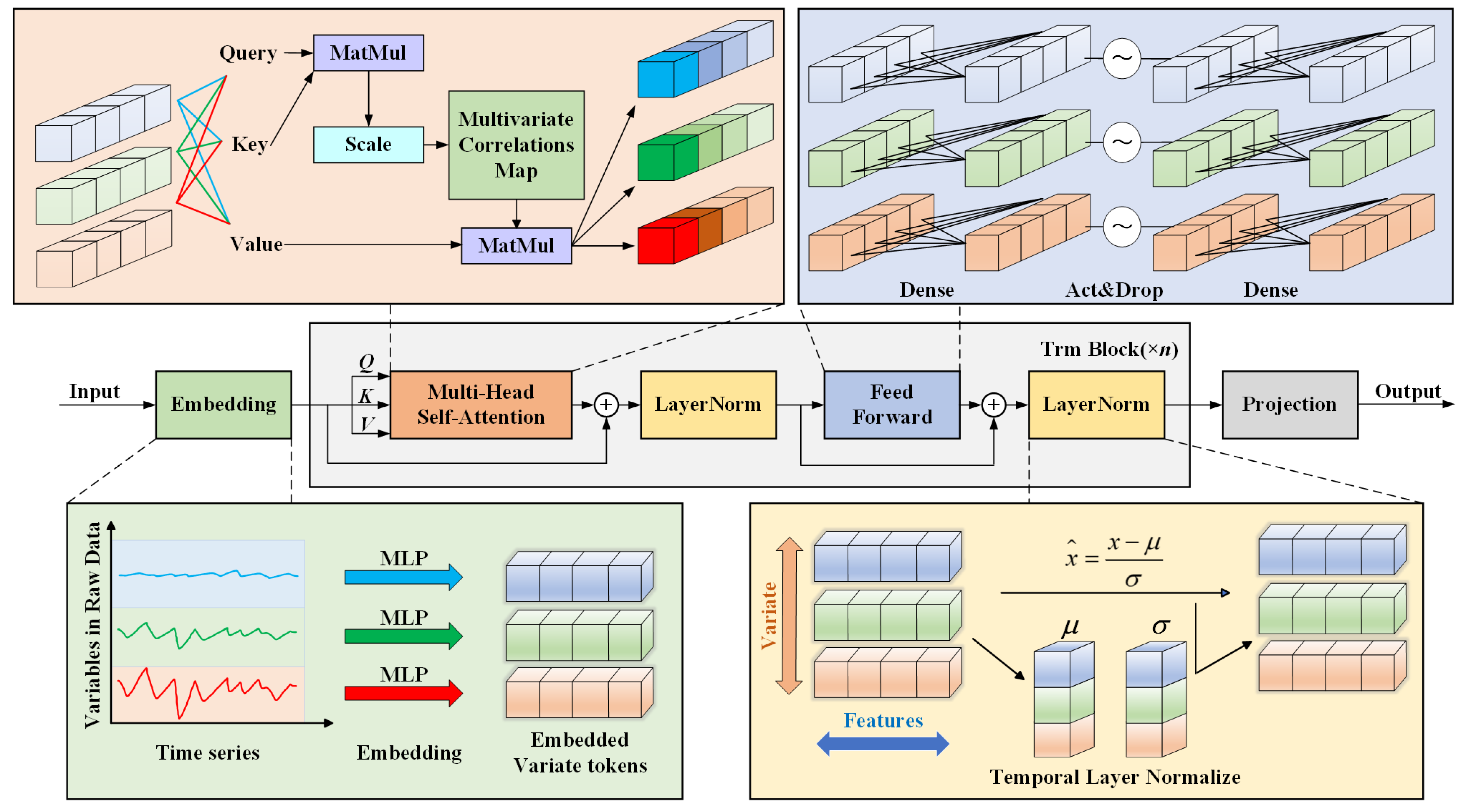
3.4. Dynamic Modeling Based on iTransformer

iTransformer is an enhanced Transformer [26,27] variant and excels in capturing long-range dependencies and hierarchical patterns. The model framework of iTransformer [28] is shown in Figure 3. iTransformer achieves greater efficiency and scalability through an innovative attention mechanism and optimized architecture. The calculation steps are summarized as follows.

Step 1: Input embedding based on variables. The input of the embedding process is defined as $\mathit{X}\in {ℝ}^{T\times M}$, T is the time step length of the input, and M is the number of features selected via NMI algorithm. Compared with Transformer, iTransformer adopts an alternative approach by embedding each series individually into a univariate token:

$${\mathit{H}}^0=MLP\left(\mathit{X}.\mathrm{transpose}\right)$$

(5)

where ${\mathit{H}}^0\in {ℝ}^{M\times D}$ represents variate token set. Using Multi-Layer Perceptron (MLP), the input length for each feature changes from T (length of time step) to D (token dimension). X.transpose means the matrix transposition operation for X.

Step 2: Run Trm blocks n times. Each time, the steps given below are performed.

Multi-head self-attention (Self_Attn) with residual connections and layer normalization (LayerNorm) is first applied on variate tokens:

$${\mathit{H}}^{l-1}=LayerNorm\left({\mathit{H}}^{l-1}+Self\_Attn\left({\mathit{H}}^{l-1}\right)\right)$$

(6)

Secondly, feed-forward network (Feed_Forward) with residual connections and layer normalization is conducted:

$${\mathit{H}}^l=LayerNorm\left({\mathit{H}}^{l-1}+Feed\_Forward\left({\mathit{H}}^{l-1}\right)\right)$$

(7)

where $l=1,2,\cdots ,n$. ${\mathit{H}}^l\in {ℝ}^{M\times D}$ is the variate token set of the l-th iteration.

Step 3: Project the variate token set to the predicted series using MLP:

$$\widehat{\mathit{Y}}=\left(MLP\left({\mathit{H}}^n\right)\right).transpose$$

(8)

4. Results and Discussion

4.1. Impact of Data Denoising

When performing deep and flexible load adjustments for the power grid, the operating conditions of CFB boilers are highly complex and variable. This leads to the presence of significant noise in the collected operational data. Noise refers to irrelevant, erroneous, or inaccurate information within the data which can negatively impact the training and prediction performance of models, ultimately leading to reduced model accuracy. To ensure the high quality of the dataset, denoising is essential. Denoising involves decomposing the data signal into multiple modal components, such as low-frequency and high-frequency components, and removing the components with the lowest energy. The remaining components are then reconstructed into a new dataset with reduced noise and improved quality. Typically, low-energy components represent noise in the signal, and removing these components can effectively reduce noise.

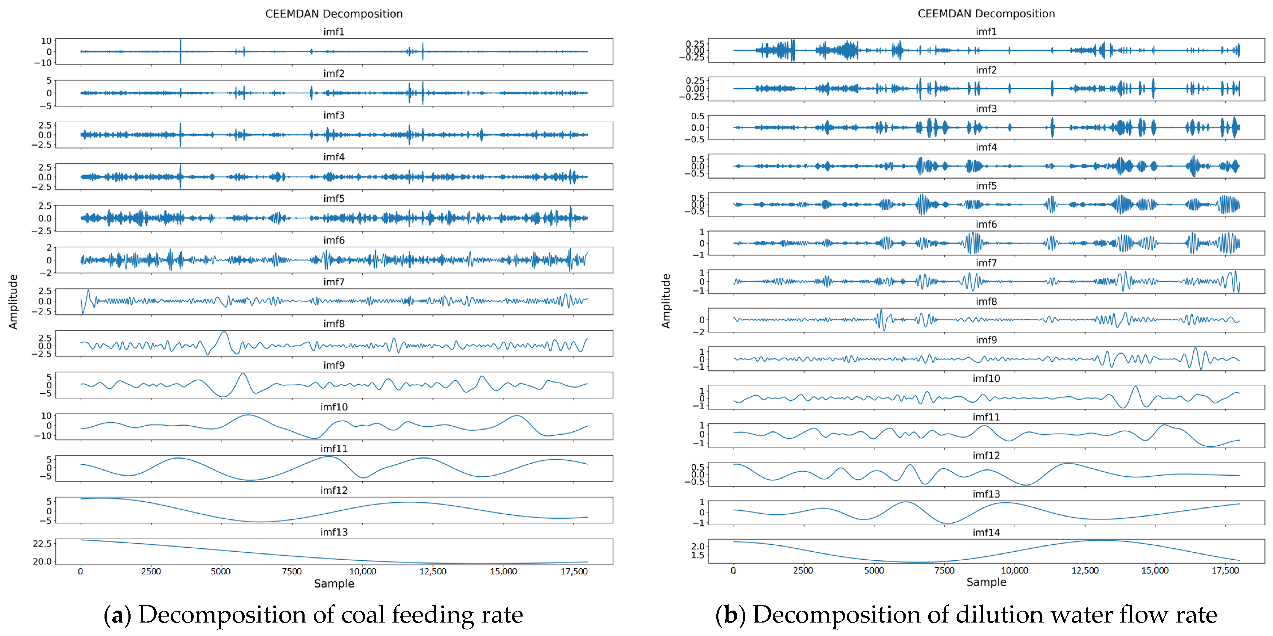
During the denoising process, the algorithm decomposes the original signal into multiple modal components, as shown in Figure 4. The energy of each component represents the signal strength and amplitude information contained in that component. The greater the energy of a component, the more it contributes to the overall signal, and it often represents the primary component or key feature. Conversely, components with lower energy contribute less and often represent noise or irrelevant variables. Figure 5 shows the energy values of these components. Determining the components to be removed is a critical aspect of data denoising. Removing too many modal components may discard useful information from the signal, causing the denoised data signal curve to deviate significantly from the original signal curve.

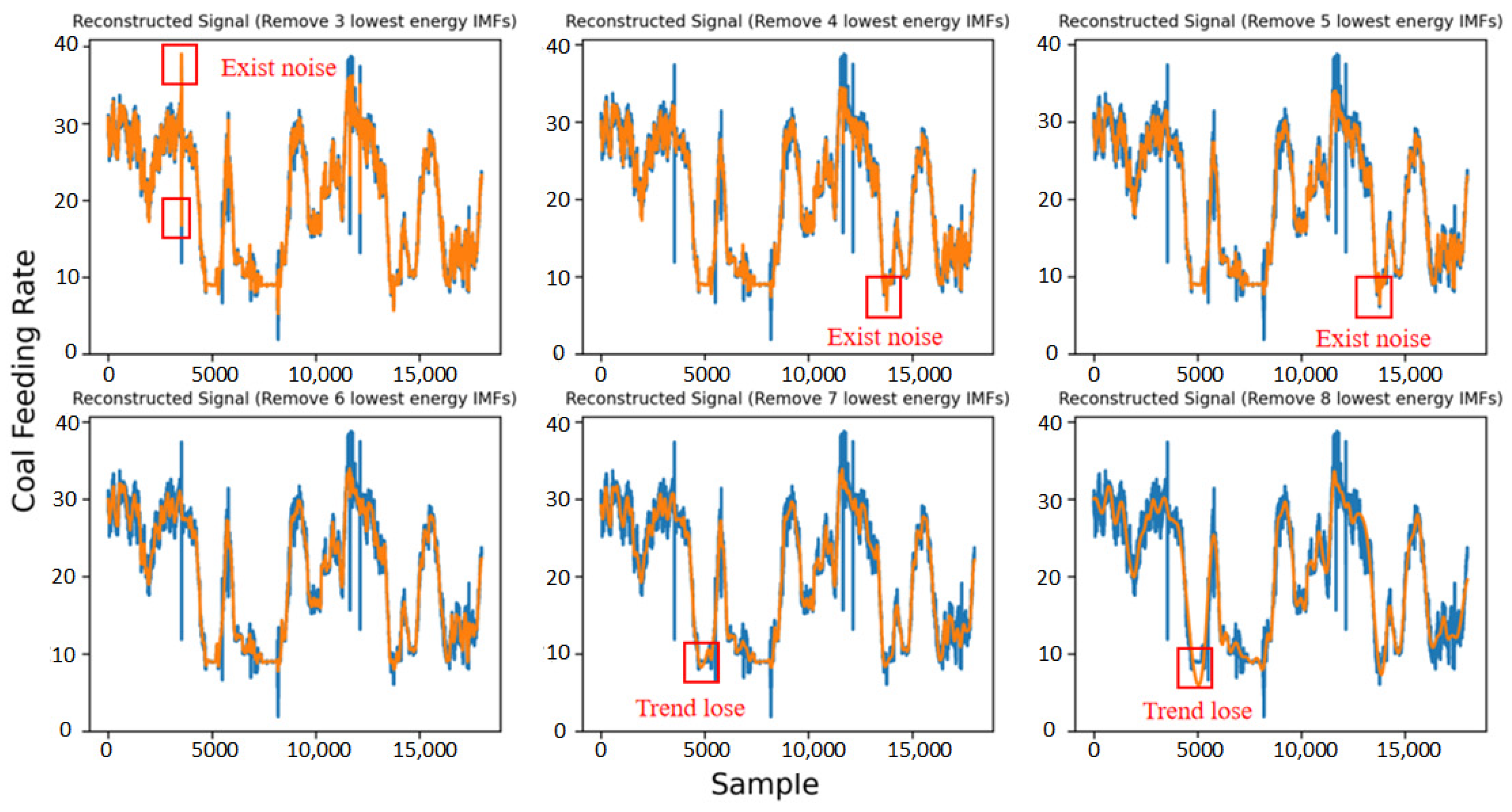
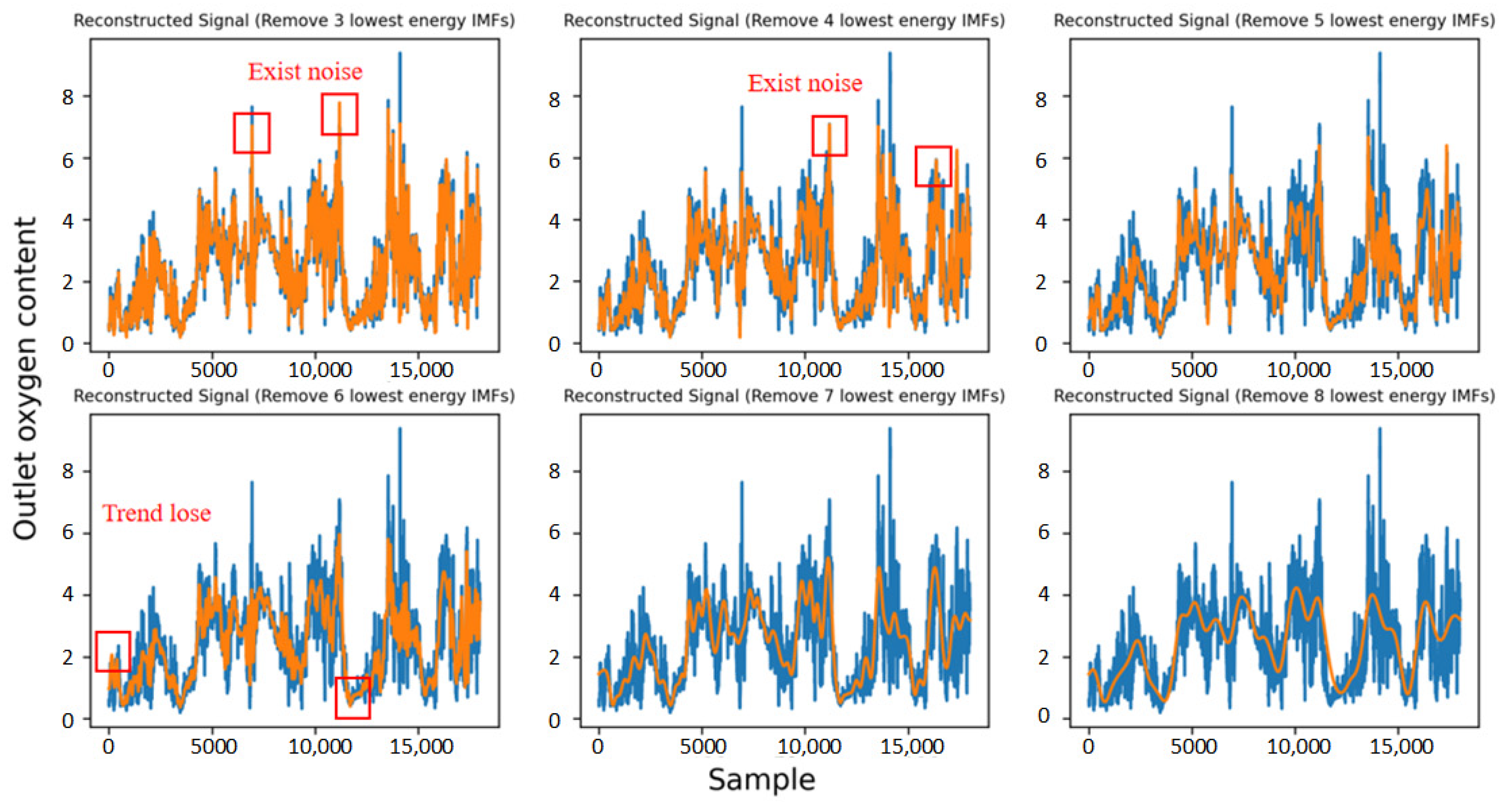
Figure 6, Figure 7, Figure 8 and Figure 9 show the comparison between the reconstructed and original signals for four different features. When denoising the “coal feeding rate” feature, reconstructing the data after removing more than six components resulted in a trend that diverges notably from the original signal, indicating that useful information is discarded. To effectively remove noise without altering the signal trend, six of the lowest-energy components are removed. Similarly, for the “SA flow rate” feature, the reconstructed curve deviates from the original signal curve when six components are removed, so five components are chosen for removal instead. Conversely, removing too few components leaves significant noise in the signal, failing to improve data quality. For the “outlet oxygen content” feature, the reconstructed data with four components removed still contains noticeable noise, while removing five components effectivity mitigates the noise and retains the signal trend.

As can be seen from Figure 6, the effect of denoising on the coal feeding rate signal is the best when the six components with the lowest energy are removed. When 3–5 components are removed, some noise is still not completely eliminated in the reconstructed signal. After more than six components are removed, the reconstructed signal has obvious signal trend loss, and the reconstructed signal has a deviation from the original signal trend.

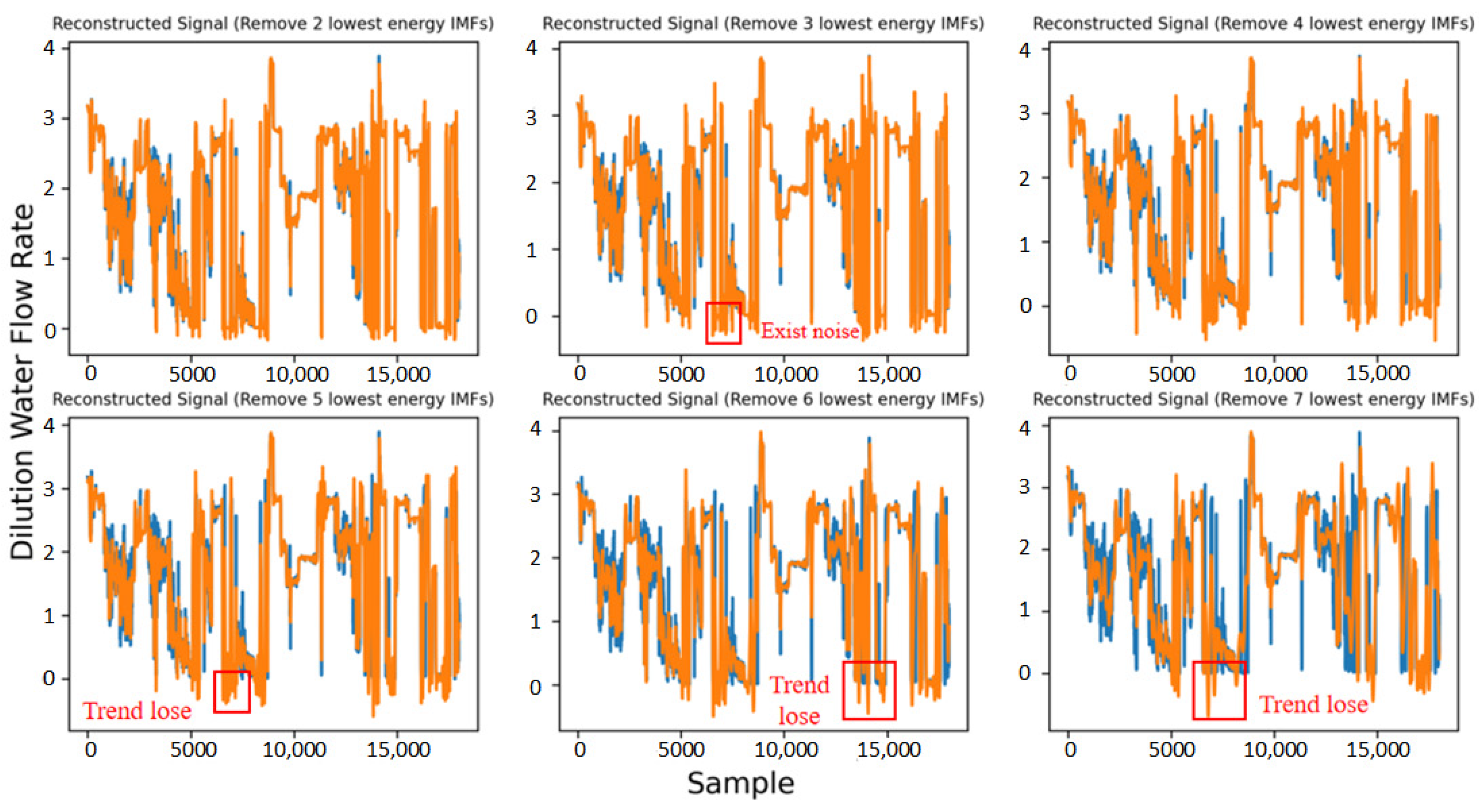
As can be seen from Figure 7, the effect of denoising on the dilution water flow rate signal is the best when the four components with the lowest energy are removed. After removing 2–3 components, there is still noise in the reconstructed signal, which will affect subsequent processing and prediction. After removing more than four components, the reconstructed signal will obviously lose the signal trend, and the reconstructed signal will lose the original signal.

As shown in Figure 8, the effect of denoising on the outlet oxygen content signal is the best when the five components with the lowest energy are removed. The noise in the reconstructed signal is still incomplete when 3–4 components are removed, which will affect subsequent work. After the removal of six components, the reconstructed signal has a tendency to be lost, and when more components are removed, the reconstructed signal obviously loses more information contained in the original signal.

It can be seen from Figure 9 that the effect of denoising is the best when the five components with the lowest energy are removed from the SA flow rate signal. There is still incomplete noise in the reconstructed signal when the 3–4 components are removed, and the effect of denoising is not the best. When six components are removed, the reconstructed signal trend is lost, and when more components are removed, the reconstructed signal curve significantly shifts more than the original signal.

The reconstructed signal curves for the different features after precise denoising are depicted in Figure 10. For the “dilution water flow rate” feature, data denoising is much more challenging since data variation is more complex, with significant fluctuations and mixed noise. To ensure there is no difference between the reconstructed and original data, four components are removed for this feature.

4.2. Analysis of Feature Selection

CFB boilers involve numerous parameters, resulting in high-dimensional field data. This high-dimensional dataset contains redundant features and features with weak correlations to the target. To prevent these irrelevant or weakly relevant features from causing model overfitting, and to avoid high computational costs and dimensionality issues associated with excessive data dimensions, it is necessary to perform feature selection. This process identifies features with strong correlations to the target and uses them as inputs for the model. In this way, the model can extract meaningful patterns from the input features, enabling accurate and efficient predictions.

The correlation between each boiler feature and the target variable was determined by the Normalized Mutual Information (NMI) values. In Figure 11, the features with NMI values greater than 0.8 have a strong correlation with the target variable (i.e., the boiler bed temperature). The results indicate that the magnitude and distribution of the Coal Seeding Air Volume play a crucial role in influencing bed temperature. The Coal Seeding Air Volume refers to the airflow responsible for transporting coal particles into the boiler. In the CFB boiler examined in this study, there are four coal feeders, each connected to two coal conveying pipelines, resulting in a total of eight pipelines labeled 11 to 18. Each pipeline is equipped with four air injection ports. For instance, pipeline 11 contains four ports, 11/11, 11/12, 11/13, and 11/14, which correspond to the 11/11 Coal Seeding Air Volume, 11/12 Coal Seeding Air Volume, 11/13 Coal Seeding Air Volume, and 11/14 Coal Seeding Air Volume, as shown in Figure 11.

Figure 12 shows the features with NMI values less than 0.8, with a red threshold line of 0.665. There is a distinct separation between features above the threshold (orange bars) and those below it (blue bars). Features above the threshold (0.665) have NMI values closer to 0.8, indicating that they are more strongly correlated with the target variable and are suitable as input features to the model.

Ultimately, the weakly correlated features corresponding to the blue bars in Figure 12 are discarded, while the strongly correlated features represented by the orange bars are selected as input features for the predictive model.

4.3. Impact of Dataset Splits

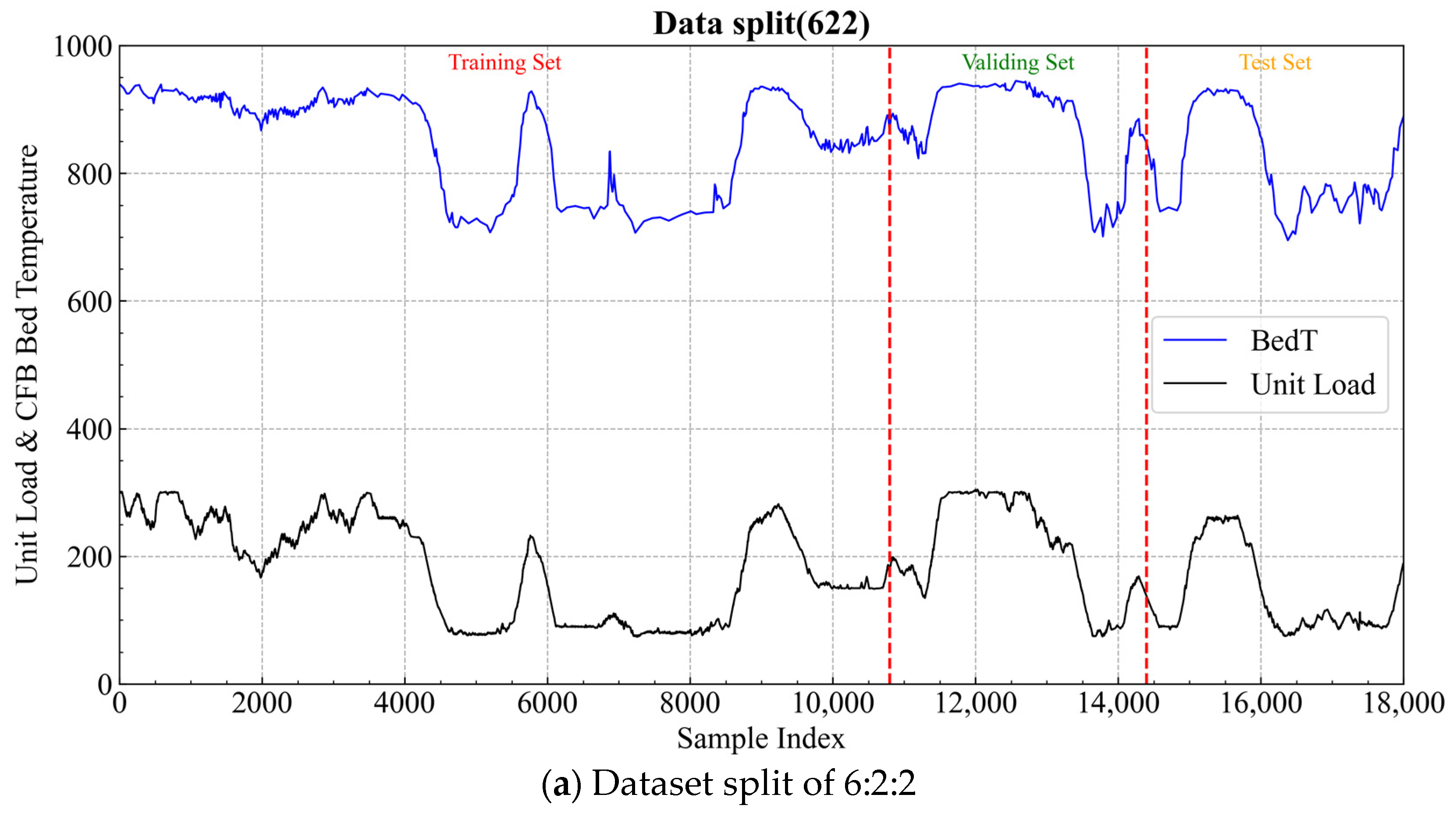
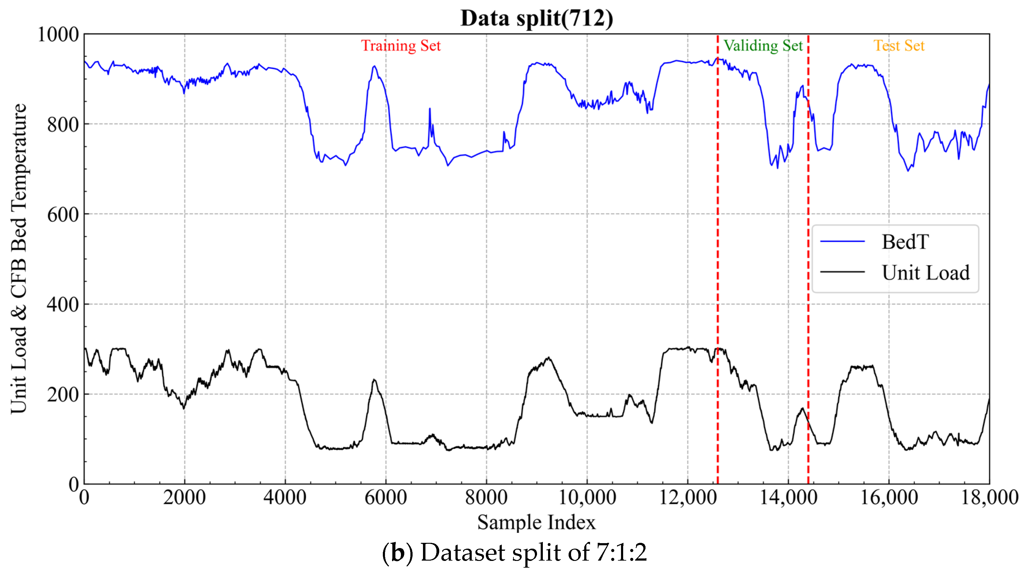
In Figure 13, the unit load refers to the power supply load of the CFB thermal power plant, which determines the boiler’s operating conditions. As shown in the figure, the dataset used in this study includes various operating scenarios, such as increasing load, decreasing load, and steady load conditions. Therefore, the data in this study can be used to validate the bed temperature prediction performance under different operating conditions. To validate the performance of the proposed prediction model, the experimental dataset is divided into training, validation, and testing sets in the ratios. If the size of the training set decreases and the model’s performance significantly deteriorates, this indicates that the model achieves high prediction accuracy only for the training data, while its generalization ability remains weak. Therefore, to investigate the impact of training data volume on the model’s generalization ability, we studied two dataset split ratios: 7:1:2 and 6:2:2 for training, validation, and testing, respectively. The 7:1:2 split, or even higher training data ratios, is a commonly adopted data partitioning method. Based on this (dataset split ratio 7:1:2), we further explored the model’s generalization ability under a lower training data ratio of 6:2:2.

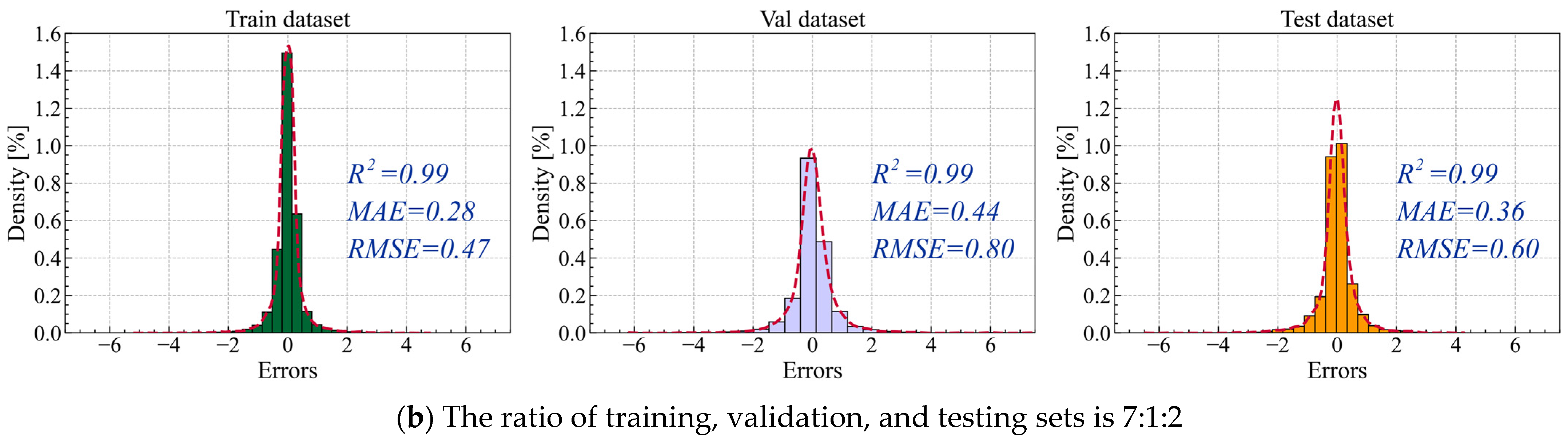
The impact of different training dataset lengths on model prediction performance is compared. Figure 14 shows the distribution of prediction errors under these two dataset splits. The results indicate that the different dataset splits have a minimal impact on prediction errors. Regardless of the dataset splits, the model’s performance across the training, validation, and testing sets remains consistent, which demonstrates the model has a strong stability and an excellent generalization ability. It is evident in Figure 14 that the proposed iTransformer model performs exceptionally well under both dataset splits, achieving an R² value of 0.99. This confirms that the model has a strong ability to capture the trends and dependencies of the input features independent of the changes in the dataset splits.

For these two data splits, the MAE changes by 0.02 mg/m³, 0.04 mg/m³, and 0.05 mg/m³ in the training, validation, and testing datasets, respectively. The RMSE changes by 0.05 mg/m³, 0.13 mg/m³, and 0.09 mg/m³ in the training, validation, and testing datasets, respectively. For metrics such as MAE and RMSE, slight fluctuations are observed due to the changes in the dataset, but they stay low and have no significant impact. The prediction model maintains consistent error levels across different datasets, proving its robust predictive performance and outstanding generalization capability.

4.4. Comparison with Other Models

Figure 15 shows the prediction effect results of the iTransformer model and other comparison models on the test set. It can be seen from Figure 15 that, on the whole, the iTransformer model performs well in terms of the trend of prediction and the change trend of measured values, while other models show obvious deviations. This shows that the forecast result of the iTransformer model is closer to the real value, and the change trend is more in line with the actual situation. Although all the models achieved a better prediction effect in the training set, the prediction effects of the comparison models were significantly worse for the new test set, which also indicated that the established iTransformer model had a strong generalization ability.

The performance of the models was evaluated based on three metrics: R², MAE, and RMSE. The results are shown in Figure 16. The iTransformer model demonstrates excellent predictive performance, achieving R² values of 0.99 across the training, validation, and testing sets. iTransformer significantly outperforms the comparative models LSTM (0.97, 0.88, 0.87) and GRU (0.96, 0.88, 0.88) and surpasses the Transformer model with the same architecture (0.98, 0.96, 0.96).

In CFB boiler operation, the bed temperature exhibits inertia, with significant long-term dependencies in the data. LSTM and GRU models fail to accurately capture these dependencies because they gradually forget previously learned information during the training process. Specifically speaking, LSTM and GRU utilize gating mechanisms to mitigate the vanishing gradient problem, but they still suffer from memory loss over long sequences. As a result, they struggle to capture long-term dependencies in CFB boiler operation data, leading to less accurate predictions. In contrast, the iTransformer and Transformer models incorporate multi-head attention mechanisms, enabling them to focus on the global information within the input data. In terms of MAE, iTransformer consistently achieves lower MAE values across all datasets compared to other models and thereby has smaller absolute errors between predicted and actual values. For the testing set, the MAE of iTransformer is 0.41 mg/m³, significantly lower than those of LSTM (20.19 mg/m³), GRU (18.8 mg/m³), and Transformer (11.77 mg/m³). Similarly, with respect to RMSE, iTransformer exhibits substantially lower values than the other models, further confirming its superior predictive accuracy and performance.

iTransformer’s advantage over Transformer lies in its treatment of variable relationships. Transformer treats multiple variables at the same time point as a single temporal token and applies attention mechanisms to derive correlations, while significant differences between variables can negatively impact its predictive performance. In contrast, the internal mechanism of iTransformer plays a crucial role in its predictive performance. By treating each variable as an independent token with a full sequence, the model effectively captures both intra-variable dependencies and inter-variable correlations. This structural design reduces interference between variables and ensures a more refined feature extraction process. The attention mechanism in iTransformer is thereby better utilized to focus on relevant long-term dependencies, leading to more stable and accurate predictions. Comparisons on the three metrics confirm that the iTransformer model exhibits outstanding predictive performance and a robust generalization ability.

4.5. Performance in Multi-Step Prediction

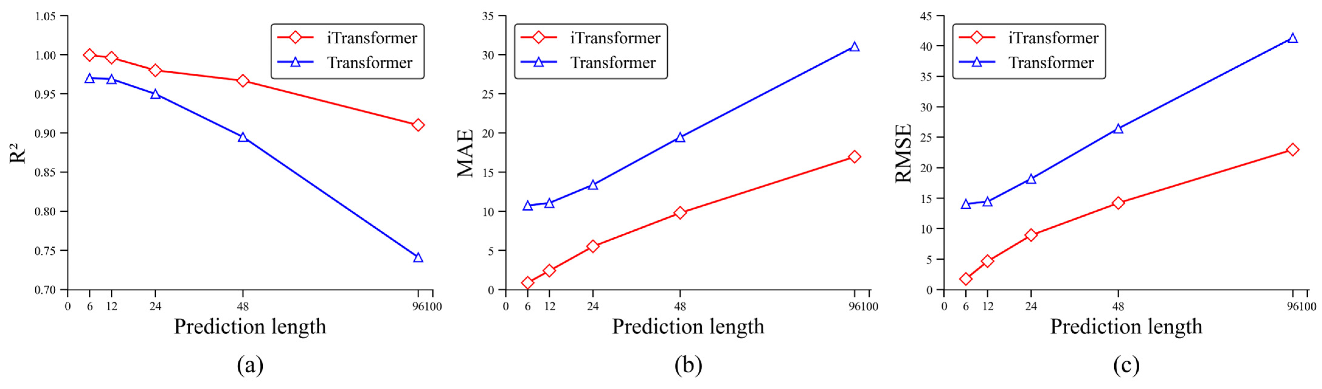
Figure 17 compares the multi-step prediction accuracy between the Transformer and iTransformer models. In the experiment, each time step corresponds to 30 s. It is necessary to explain the errors in Figure 17. The error at each point in the figure represents the error of the output sequence with that length. For example, the errors at x = 48 and x = 96 do not correspond to the errors at the 48th and 96th time steps, but rather to the errors of the output sequences predicted for the next 48 and 96 time steps, respectively.

For the testing dataset, as the number of time steps increases, the prediction errors of both models grow rapidly, resulting in reduced R². This can be attributed to two primary factors: First, Transformer-based models have already effectively handled long-term dependencies. With sufficient data and model parameters, they can achieve excellent long-range forecasting performance, similar to GPT and DeepSeek. However, in industrial applications, due to limitations in training data volume and hardware constraints such as GPUs, the model’s parameter size is restricted, leading to increased long-term prediction errors. Secondly, despite the self-attention mechanism enabling Transformer-based models to capture long-range dependencies, in time series forecasting, distant historical data often has a weaker influence on far-future predictions compared to more recent data. As a result, Transformer-based models tend to prioritize learning short-term patterns, while their ability to accurately capture long-term trends is relatively weaker, leading to a decline in predictive accuracy over longer horizons. However, iTransformer consistently achieves higher accuracy than Transformer. Notably, when predicting the next 48 time steps (24 min), iTransformer maintains an R² value above 0.95, while the R² of Transformer drops below 0.90. For iTransformer, the prediction error becomes evident after predicting the next 12 steps (6 min), so iTransformer is reliable in predicting bed temperature changes within the next 6 min with high accuracy in practical applications.

5. Conclusions

This study proposed a CEEMDAN-NMI–iTransformer framework for predicting bed temperature in utility CFB boilers, addressing challenges in data quality, feature selection, and long-term dependency modeling. The model was validated using real operational data from a 300 MW CFB boiler and outperformed traditional deep learning models in single-step and multi-step predictions. The key conclusions are as follows:

(1)

The CEEMDAN algorithm significantly enhances data quality for predictive modeling. For each feature, the appropriate components are analyzed and selected to preserve the overall signal trend while effectively removing substantial noise points.

(2)

The NMI-based feature selection reduces complexity while preserving accuracy. From 130 operational variables, the most relevant features with NMI values greater than 0.665 were chosen, enhancing computational efficiency. This process also emphasizes key factors, such as the magnitude and distribution of the coal seeding air, that play a crucial role in the system’s performance.

(3)

The iTransformer model outperforms LSTM, GRU, and Transformer, achieving an R² of 0.99 for single-step predictions across different training dataset sizes, and maintaining an R² above 0.95 for 24 min forecasts, demonstrating superior capability in capturing long-term dependencies.

Our future work will enhance the iTransformer model with adaptive attention mechanisms to dynamically adjust feature importance in real time, improving its ability to handle nonlinear fluctuations and sudden operational changes in CFB boilers, further strengthening prediction accuracy, robustness, and generalization.