Abstract
Lost circulation is a major challenge in the drilling process, which seriously restricts the safety and efficiency of drilling. The traditional monitoring model is hindered by the presence of noise and the complexity of temporal fluctuations in lost circulation data, resulting in a suboptimal performance with regard to accuracy and generalization ability, and it is not easy to adapt to the needs of different working conditions. To address these limitations, this study proposes a multi-scale feature fusion model based on wavelet transform and TimeGAN. The wavelet transform enhances the features of time series data, while TimeGAN (Time Series Generative Adversarial Network) excels in generating realistic time series and augmenting scarce or missing data. This model uses convolutional network feature extraction and a multi-scale feature fusion module to integrate features and capture time sequence information. The experimental findings demonstrate that the multi-scale feature fusion model proposed in this study enhances the accuracy by 8.8%, reduces the missing alarm rate and false alarm rate by 12.4% and 6.2%, respectively, and attains a test set accuracy of 93.8% and precision of 95.1% in the lost circulation identification task in comparison to the unoptimized model. The method outlined in this study provides reliable technical support for the monitoring of lost circulation risk, thereby contributing to the enhancement of safety and efficiency in the drilling process.
1. Introduction
Conventional oil and gas resources are a subject of continuous development, and the oil and gas exploration and development industry is gradually expanding towards complex oil and gas fields such as unconventional, deep, and deep sea, which are rich in resources. Wellbore circulation fluid loss is caused by a variety of factors, which are generally linked to four geological formations [1]: porous matrix, massive cavities, naturally occurring fractures, and drilling-induced fractures [2]. Complex oil and gas formations with high temperature and high pressure, complex layers, and easy instability lead to high leakage risk and strong concealment. The challenge of identifying these risks is further compounded by the presence of data noise, real-time fluctuations, and nonlinear mapping relationships [3]. If these risks are not detected in a timely manner, resulting in processing lag, the consequences can be severe, including the potential for malignant leakage and well-blowout accidents. Consequently, the accurate and effective monitoring of lost circulation risk is of paramount importance for ensuring the safety and efficiency of drilling operations.
At present, the field of lost circulation diagnostics can be divided into two broad categories: traditional methods and methods based on intelligent technologies. Engineers reliant upon traditional methods utilize sensor equipment to monitor real-time fluctuations of key parameters in the drilling process in order to make judgments regarding lost circulation [4]. However, such traditional methods are limited by the measurement accuracy of the sensors and the experience level of the engineers; moreover, the accuracy and timeliness of these methods are often insufficient. In recent years, with the advent of deep learning technology, the focus of research in lost circulation diagnosis has shifted towards monitoring methods based on intelligent algorithms. For instance, in 2016, Simeng Han et al. [5] explored real-time early warning methods for drilling overflows and constructed a real-time early warning model based on the sign parameters through BP neural networks. In 2018, the research team led by Al-Hameedi et al. [6] proposed a partial least squares regression method to estimate wellbore losses during drilling operations. By utilizing the Variable Importance in the Projection approach, they identified key drilling parameters that significantly influenced the model, providing a quantitative basis for optimizing drilling operations. In 2023, Yan Yan’s team [7] applied the risk trend line method to improve the early warning capability of drilling overflow and lost circulation risk. In the same year, Zheng Zhuo’s team [8] utilized the XGBoost algorithm to construct a lost circulation warning model for the Bohai Oilfield, achieving an accuracy of 87%. Sun Weifeng’s team [9] proposed a lost circulation monitoring method based on DCC-LSTM. DCC-LSTM (Dynamic Conditional Correlation Long Short-Term Memory network) is an advanced time series prediction model that effectively captures the dynamic correlations between multidimensional data, making it particularly suitable for complex data analysis in lost circulation monitoring. They improved the accuracy of lost circulation incident prediction to 75% while simultaneously reducing the false alarm rate. These methodologies are adept at handling substantial data volumes and identifying anomalies through automated models. Nevertheless, the inability of features to adequately characterize the lost circulation state under the prevailing data conditions, in conjunction with the paucity of valid lost circulation samples, constitute the primary constraints on the efficacy of intelligent models [9].
In the field of lost circulation detection, effective lost circulation data features typically contain complex information in both the time and frequency domains. However, existing models have limited capabilities in extracting these complex features, and the scarcity of valid lost circulation samples significantly constrains the performance of intelligent models. Therefore, this study proposes a multi-scale feature fusion model that combines wavelet transform and TimeGAN. The model not only extracts multi-scale time series features from lost circulation data using wavelet transform but also generates new samples with TimeGAN to address the issue of insufficient samples. The optimal feature fusion strategy is obtained through the multi-scale feature fusion module, which enhances both diagnostic accuracy and stability. This method not only overcomes the data scarcity problem in lost circulation detection but also thoroughly explores the temporal and frequency features in lost circulation data, providing an efficient and accurate solution for monitoring lost circulation risks while reducing reliance on a large amount of labeled lost circulation data.
2. Methodology
2.1. Wavelet Transform
Wavelet transform (WT) is a tool for analyzing signals in the time and frequency domains [10], which is widely used in fields such as noise removal and pattern recognition. Its basic formula is:
where are the wavelet coefficients, is the signal to be analyzed, is the mother wavelet function, and a and b denote the scale and translation parameters, respectively. The scaling parameter a governs the range of frequency analysis, while the translation parameter b determines the temporal position within the signal.
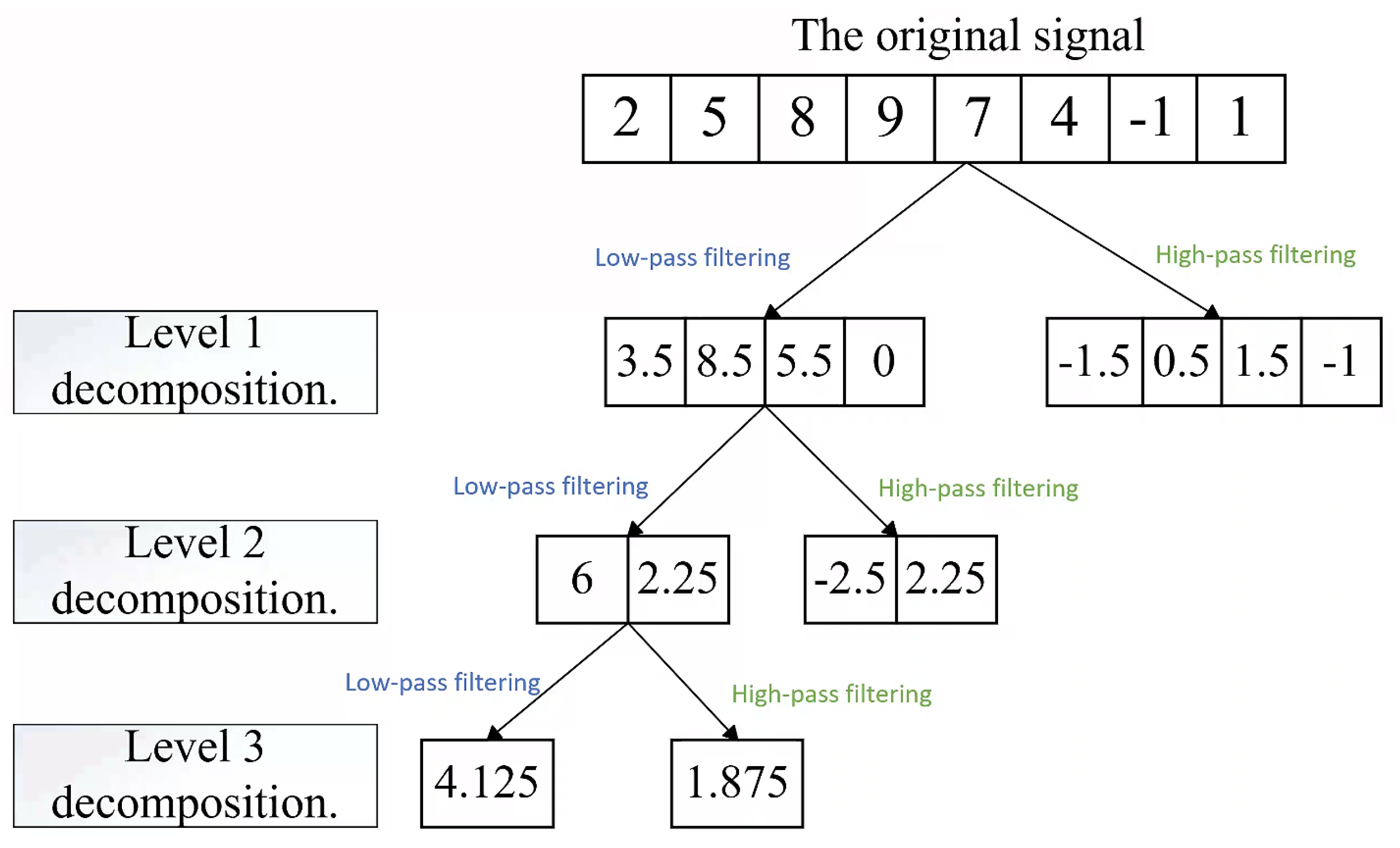
The wavelet transform method is utilized to process the original feature signal, with the signal initially decomposed into low-frequency approximation and high-frequency details. A further decomposition of the low-frequency approximation and high-frequency details into low-frequency approximation and high-frequency details follows this. Subsequent decomposition of the resultant part of the last decomposition is then performed into low-frequency approximation and high-frequency details, with each part of the decomposition subdivided individually until each part of the decomposition is limited to a single point. The high-frequency details part is not decomposed, and the decomposition steps are illustrated in Figure 1. The application of wavelet transform facilitates the division of the signal into multiple scales, thereby enabling the analysis of the information of the target signal in each frequency band with greater precision and facilitating a comprehensive exploration of the intrinsic law of the signal.
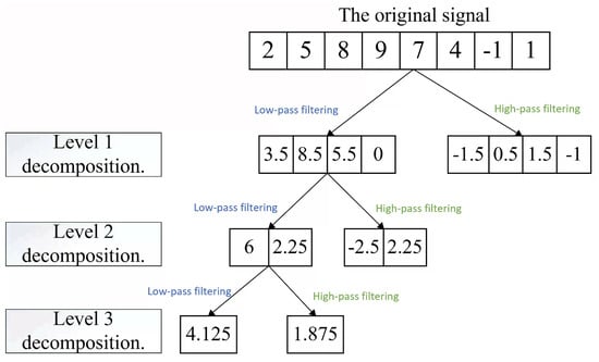
Figure 1.
Schematic of wavelet multilevel decomposition.
2.2. TimeGAN
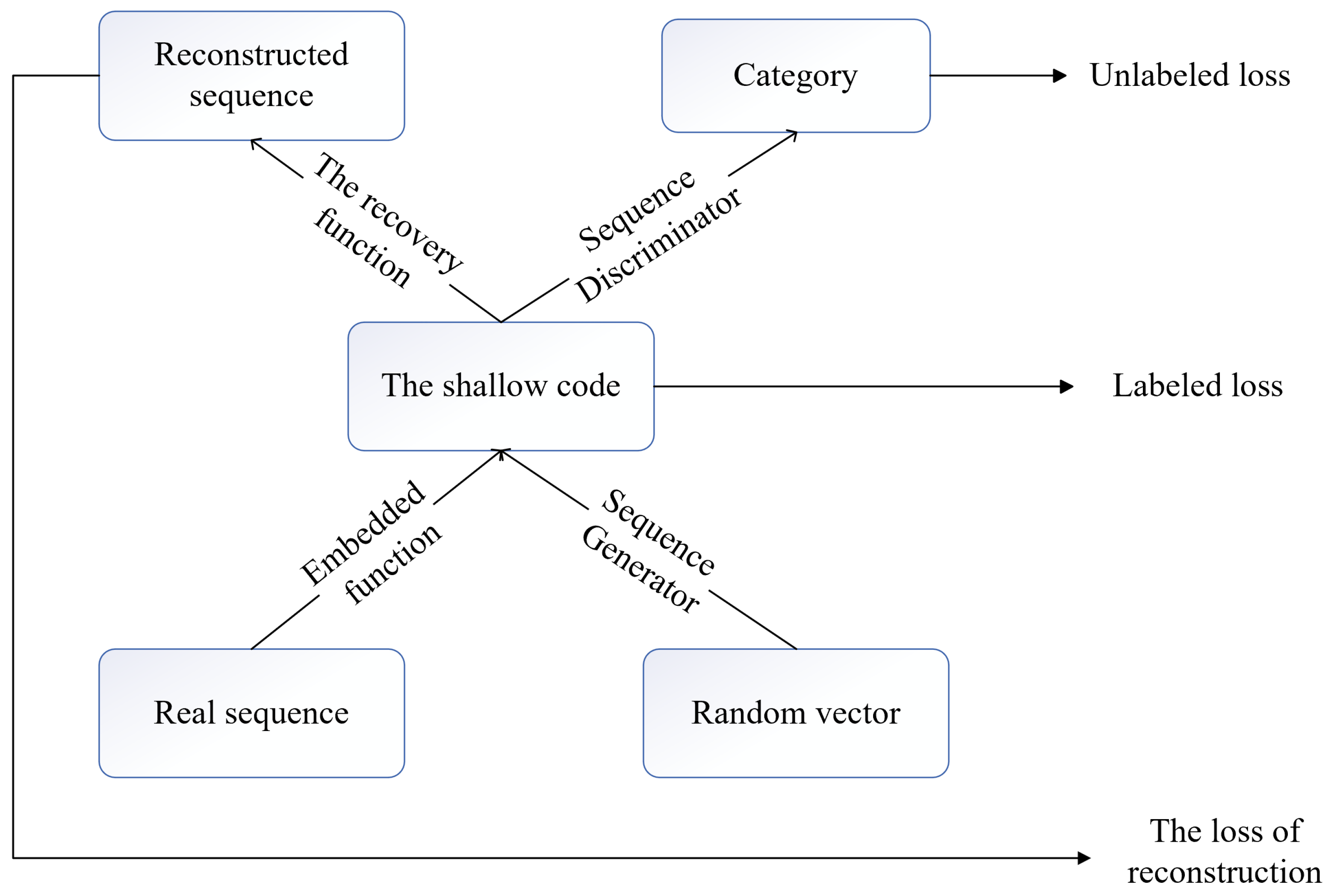
The training process of GAN is an adversarial process, where the generator and the discriminator compete with each other in a game. In this game, the generator tries to generate more and more realistic counterfeit data while the discriminator tries to distinguish between real data and counterfeit data as accurately as possible. The adversarial mechanism drives the generator and discriminator to continuously optimize through dynamic interplay, forcing the generated data distribution to approximate real data, achieving high-quality sample generation. The enhancement of TimeGAN [11] is attributable to its comprehension of two pivotal characteristics of temporal data: namely, the static features, which remain constant over time, and the temporal features, which change over time. The TimeGAN network comprises four constituent elements: the embedding function, the recovery function, the sequence generator, and the sequence discriminator. The configuration of this network is illustrated in Figure 2.
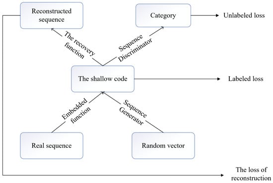
Figure 2.
TimeGAN components.
The embedding function maps raw risk time series data into a low-dimensional latent space, with its core objective being to capture temporal correlations and long-range dependency features in lost circulation events. The recovery function reconstructs original data or generates new samples from latent space vectors, typically forming an encoder–decoder architecture with the embedding function. The sequence generator employs adversarial training strategies to synthesize time series data with lost circulation risk characteristics in the latent space, capturing sequence dependencies through autoregressive or parallel prediction. The sequence discriminator evaluates the authenticity of the generated sequences via adversarial training or classification mechanisms, driving generator optimization through distribution matching. The embedding and recovery functions constitute an autoencoder that constrains the reversibility and compact distribution of the generated data, while the generator and discriminator utilize adversarial learning to force the synthetic data to approximate the statistical properties of real lost circulation time series. This framework addresses the data scarcity issue in small-sample risk scenarios and provides high-fidelity training data for risk prediction models.
The auto-coding component of TimeGAN is capable of realizing the inverse mapping between feature space and potential space and can reconstruct the data according to the potential static and temporal features of the real data. The mathematical expressions for the reconstruction loss function , the unsupervised loss function , and the additional supervised loss function during training are as follows.
where and denote the static and temporal feature vectors of the generated data, S and denote the static and temporal feature vectors of the real data, and denote the static and temporal feature vectors of the latent layer feature space, and denote the discriminator’s discriminant values for the static and temporal feature vectors (Table 1).

Table 1.
Comparison of loss functions: core functions and technical specifications.
2.3. Multi-Scale Feature Fusion Neural Network Structure
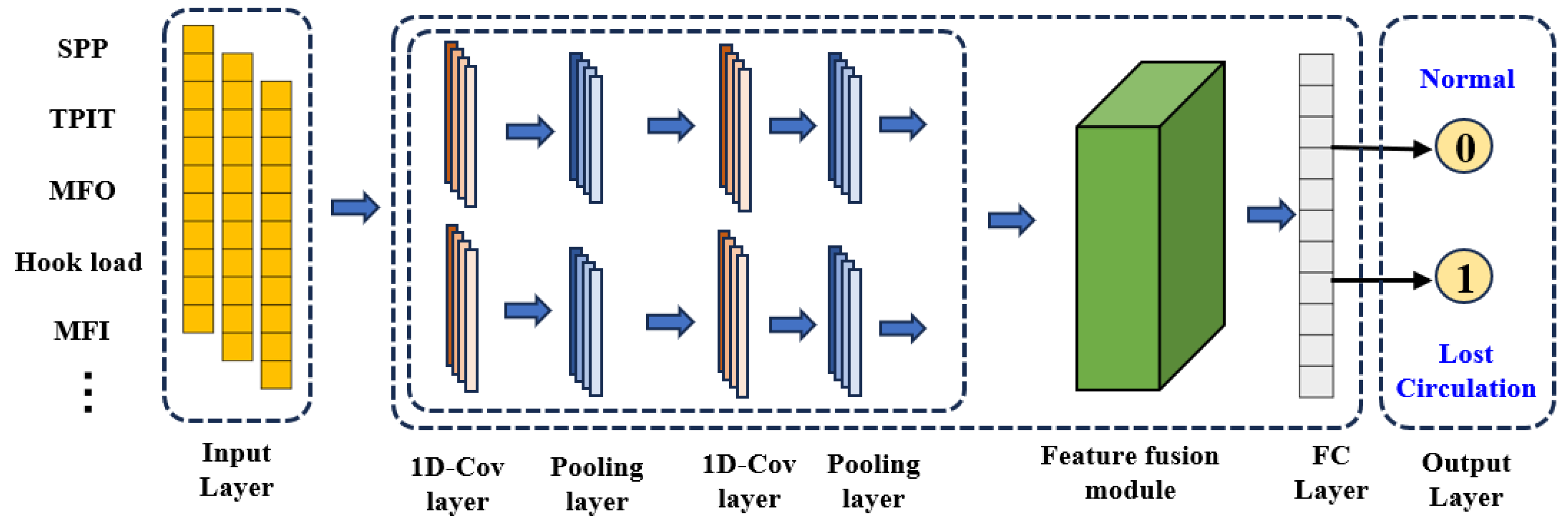
The core structure of the network is divided into three parts: a feature extraction module constructed from a convolutional neural network, a feature fusion module for multi-scale feature fusion, and a detection classifier consisting of a fully connected layer [12]. The input features of the network include expanded lost circulation data and multiple features after wavelet transform.
The initial extraction of features is accomplished through the utilization of the larger convolution of the convolution kernel, thereby facilitating the filtration of noise interference in the time series data [13]. The feature extraction backbone network executes the initial processing and feature extraction of the input data. In comparison with the conventional feature extraction network, the parallel feature extraction approach can enhance the feature extraction capability of the model without an increase in complexity [14].
As the various evaluation factors contain rich and complex information, the multi-scale feature fusion model for lost circulation prediction, based on wavelet transform and TimeGAN, extracts feature information through a single scale. This results in insufficient feature mining and inaccurate forecasts of lost circulation. In order to overcome these challenges, a multi-scale feature fusion model has been created, as shown in Figure 3.
The multi-scale feature fusion model primarily employs convolutional layers to extract local temporal features from signals. These local features are then fed into a bidirectional GRU network (as shown in Equation (7)), where gated recurrent units capture the signal’s long-term temporal dependencies. The corresponding mathematical formulations are provided in Equations (5)–(7).
where denotes the ReLU activation function; , , and denote the weight matrices corresponding to the convolutions Convl, Conv2, and Conv3, respectively; , , and denote the bias values corresponding to the above convolutions, respectively; and denotes the signal input into the gated loop unit.
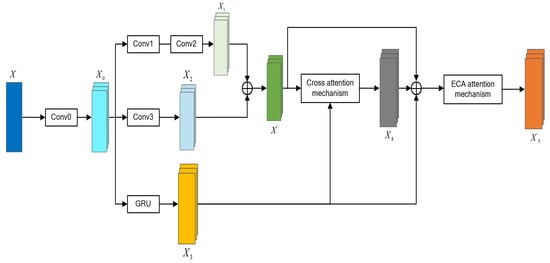
Figure 3.
Multi-scale cross-feature fusion module.
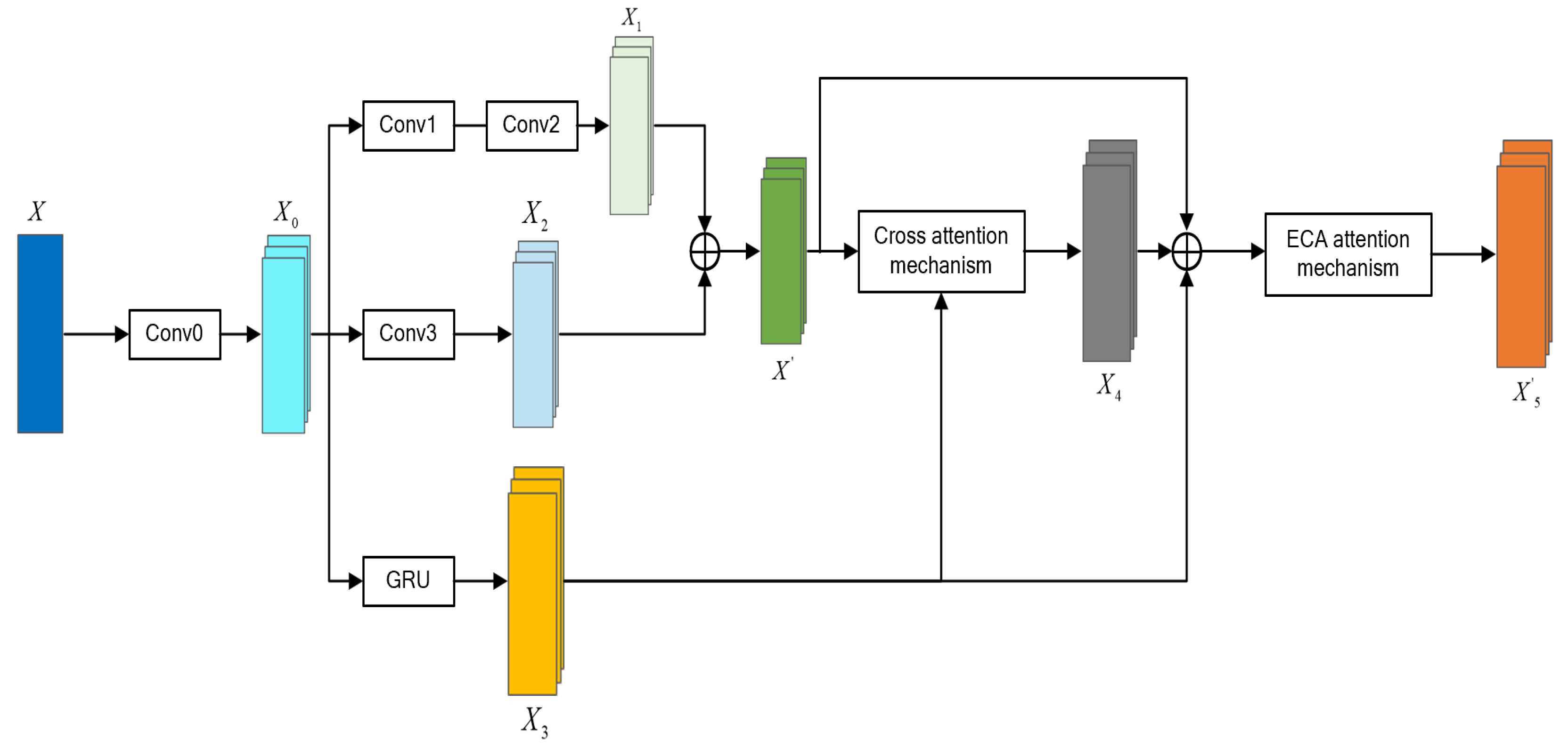
Each layer uses the attention mechanism to dynamically adjust the feature weights to achieve an adaptive allocation of the importance of different features. Specifically, the multi-layer fusion module fuses the expanded lost circulation data and wavelet-transformed features at various levels, highlighting key information and suppressing redundant or irrelevant features through the attention mechanism. For different scales of local time features and long-time-dependent features, the local time features are summed to obtain , and cross attention is calculated with to obtain the fusion feature information.
Following the acquisition of the enhanced features, these are input into the fully connected layer for the prediction of target information. The detection classifier outputs the probability of lost circulation occurring through the fully connected layer, and the output result is a binary classified lost circulation probability between 0 and 1. Regarding the loss function, the error is calculated using the mean square error, and the output lost circulation probability is used as binary cross-entropy. The entire convolutional neural network structure is shown in Figure 4.

Figure 4.
Multi-layer dynamic feature weight neural network structure.
3. Data Processing
3.1. Feature Selection
In this study, the Spearman correlation coefficient method is utilized to optimize the feature set selection process, with consideration given to the data characteristics and computational efficiency.
The method is particularly well-suited to non-normally distributed data. The formula for calculating the Spearman correlation coefficient is as follows:
where is the final Spearman correlation coefficient value taken by the two variables, n is the number of data in the variable, and is the square of the difference in the rank order of the data of the two variables.
In this study, the Spearman correlation coefficient between each characteristic parameter and the lost circulation label is calculated, and the results are shown in Figure 5.
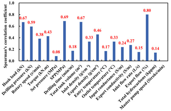
Figure 5.
Characteristic correlation coefficient calculation results.
Following a thorough examination of the available domain knowledge, in conjunction with the analysis of expert experience and feature preference, seven parameters were selected as the input features for the intelligent model: hook load, drilling pressure, torque, riser pressure, TPIT, outlet density, and MFO. It was determined that MFO, SPP, and TPIT exhibited a high correlation with lost circulation labeling. Furthermore, these parameters were found to be consistent with field engineering practice and expert experience.
3.2. Data Cleaning
This study uses time series data from 13 wells in real drilling sites of offshore oil fields in China, with a data acquisition interval of 5 s, totaling over 300,000 normal data points and more than 5000 lost circulation data points. Specifically, these raw data cover key variables such as different lithologies, formation pressure gradients, well depth ranges and working conditions. The raw data contain anomalies and missing values. In order to screen the abnormal values, this study adopts the improved sliding window 3 method and sets the appropriate window size to avoid misjudging the normal data. The outliers are replaced with null values, which are subsequently filled by spline interpolation to preserve the overall trend of the data. This study applies smoothing filtering to the data, using the average of the current point and the previous 99 points to smooth each data point, which helps reduce noise and improve data quality. Finally, the maximum–minimum normalization method was used to make the data dimensionless, with the intention of shortening the model training time and reducing overfitting. The relevant formula, Formula (9), is as follows:
where x is the data sample, is the normalized value of x, and and are the maximum and minimum values of the variable x.
3.3. Sample Construction
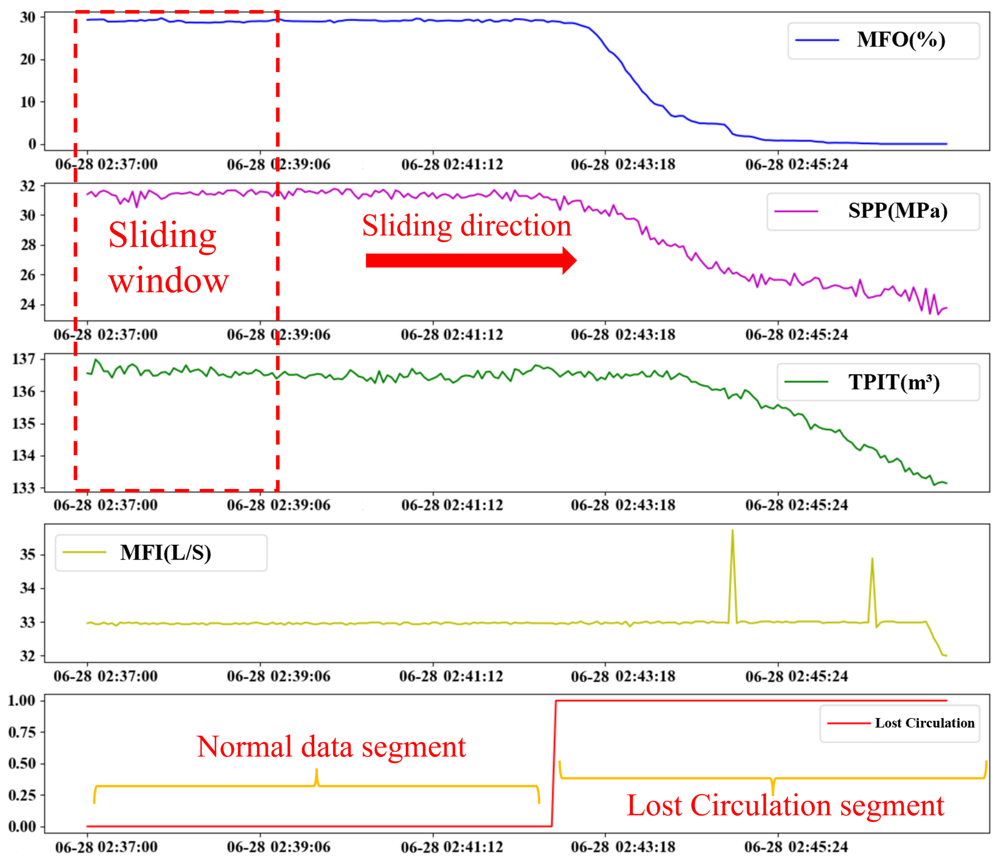
In this study, the sliding window method is used to construct fixed-length lost circulation time series samples, as shown in Figure 6. Under the premise of maximizing the use of data, the window sliding step is set to 1, and the window length can be adjusted according to the modeling effect. In order to ensure that the sample has effective features, the window length is usually not less than 30 data points.

Figure 6.
Time series sample construction based on sliding window method.
3.4. Wavelet Transform-Based Temporal Feature Enhancement
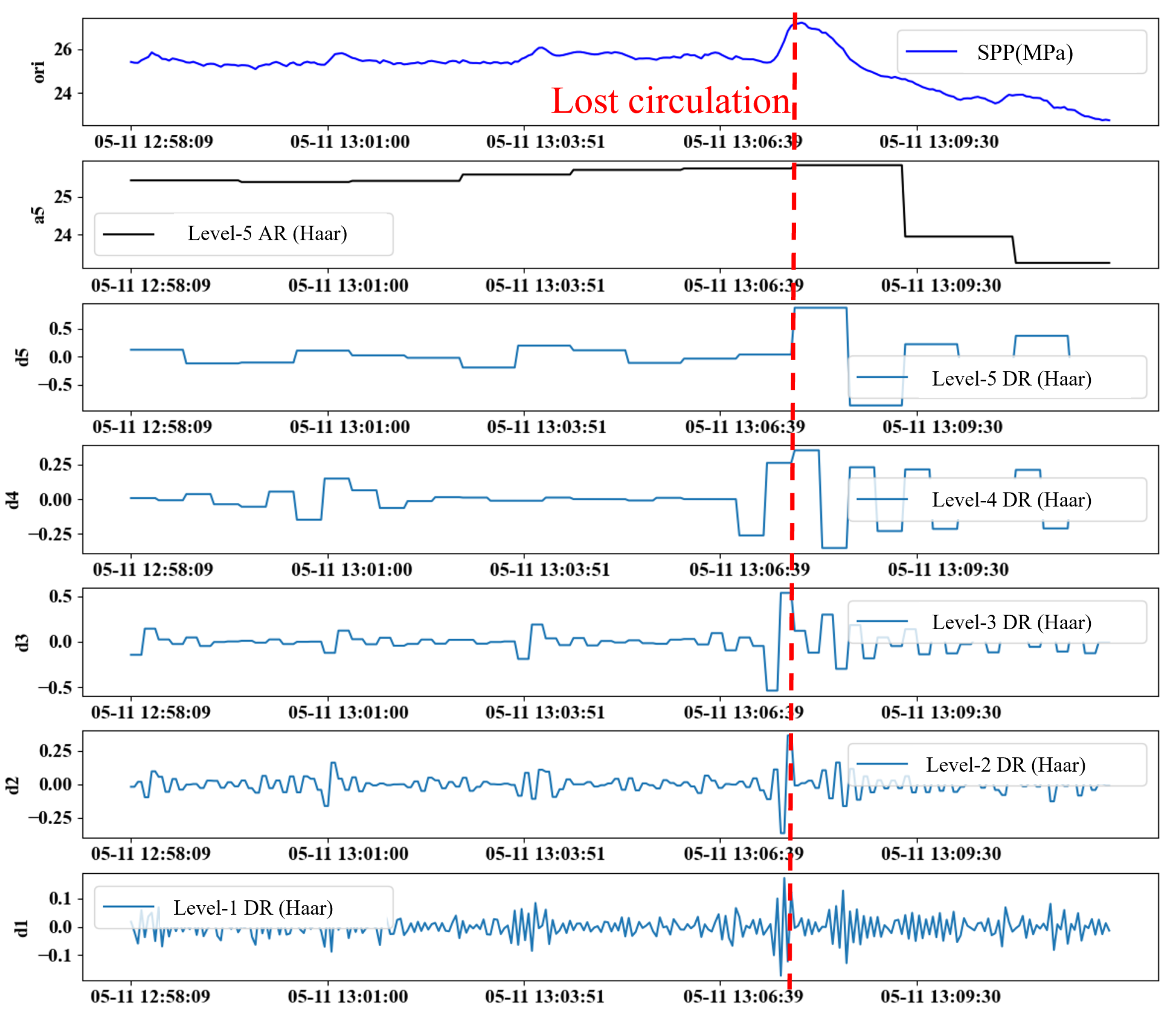
The key factors of the wavelet transform effect are the number of wavelet decomposition layers and the type of wavelet function, and the selection of appropriate parameters can significantly improve the transform effect. According to the characteristics of the lost circulation time series data, this study adopts the Haar wavelet function to transform the original feature signal and sets the number of decomposition layers to 5. Taking SPP as an example, the result after its reconstruction with five levels of decomposition is shown in Figure 7, where the low-frequency approximate features are similar to the original features, while the high-frequency detail features (d1∼d5) show different degrees of oscillation characteristics.
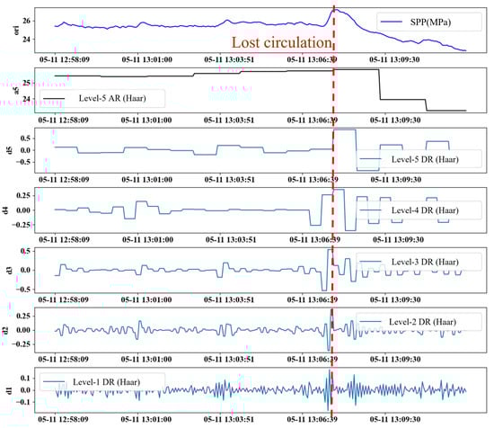
Figure 7.
Haar five-level wavelet decomposition reconstruction for SPPs.
Among the high-frequency detail features, the oscillation frequencies of d1 and d2 are higher, but the difference is not obvious, and the oscillation patterns of d4 and d5 exhibit excessive discreteness, rendering them inadequate for effectively capturing the continuous variations that occur before and after the onset of lost circulation. In contrast, d3 achieves a better balance between signal continuity and amplitude fluctuation characteristics and is able to more clearly characterize the data fluctuations before and after the lost circulation. Therefore, the 3-level wavelet decomposition is the most effective.
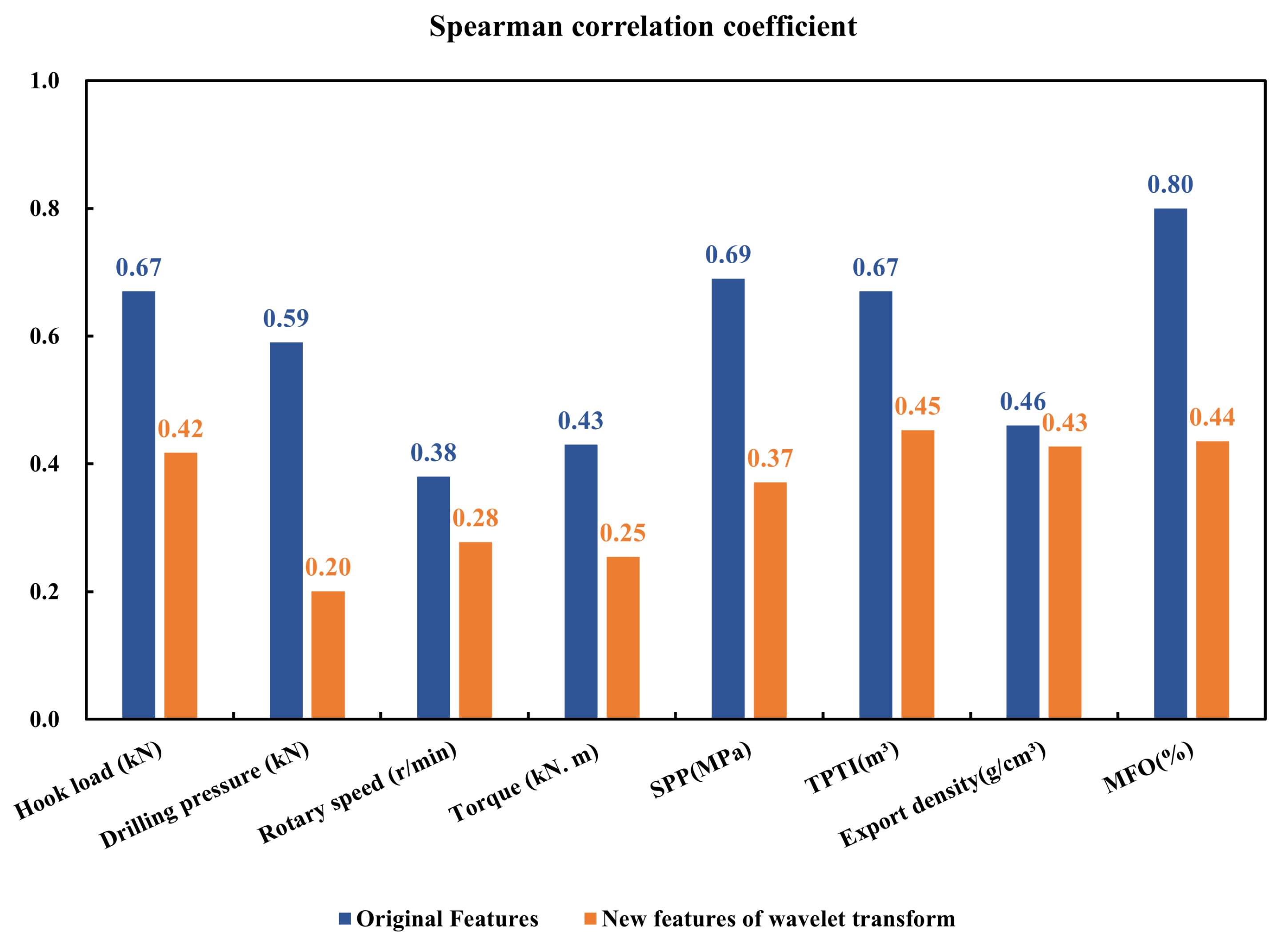
After wavelet transforming the seven lost circulation time series features, the correlation between the new features and the lost circulation labels is analyzed by the correlation coefficient method, and the results are shown in Figure 8. Although the Spearman correlation coefficients of the new features have decreased, the transformed features of Hook load, SPP, TPIT, and MFO are still strongly correlated with the lost circulation risk labels, and these four features are finally selected as the effective enhancement features of the lost circulation risk.

Figure 8.
Spearman correlation coefficients of specific features (e.g., SPP, MFO) before and after wavelet transformation.
3.5. TimeGAN-Based Temporal Data Expansion
In order to ascertain the efficacy of the TimeGAN model in the generation of lost circulation time series data, this study uses the lost circulation time series data from the lost circulation periods in the lost circulation dataset, constructing the training set using the method mentioned in Section 3.2. In order to meet the input format requirements of the TimeGAN model, the lost circulation time series data are initially constructed into fixed-window time series samples using the sliding window method and subsequently normalized.
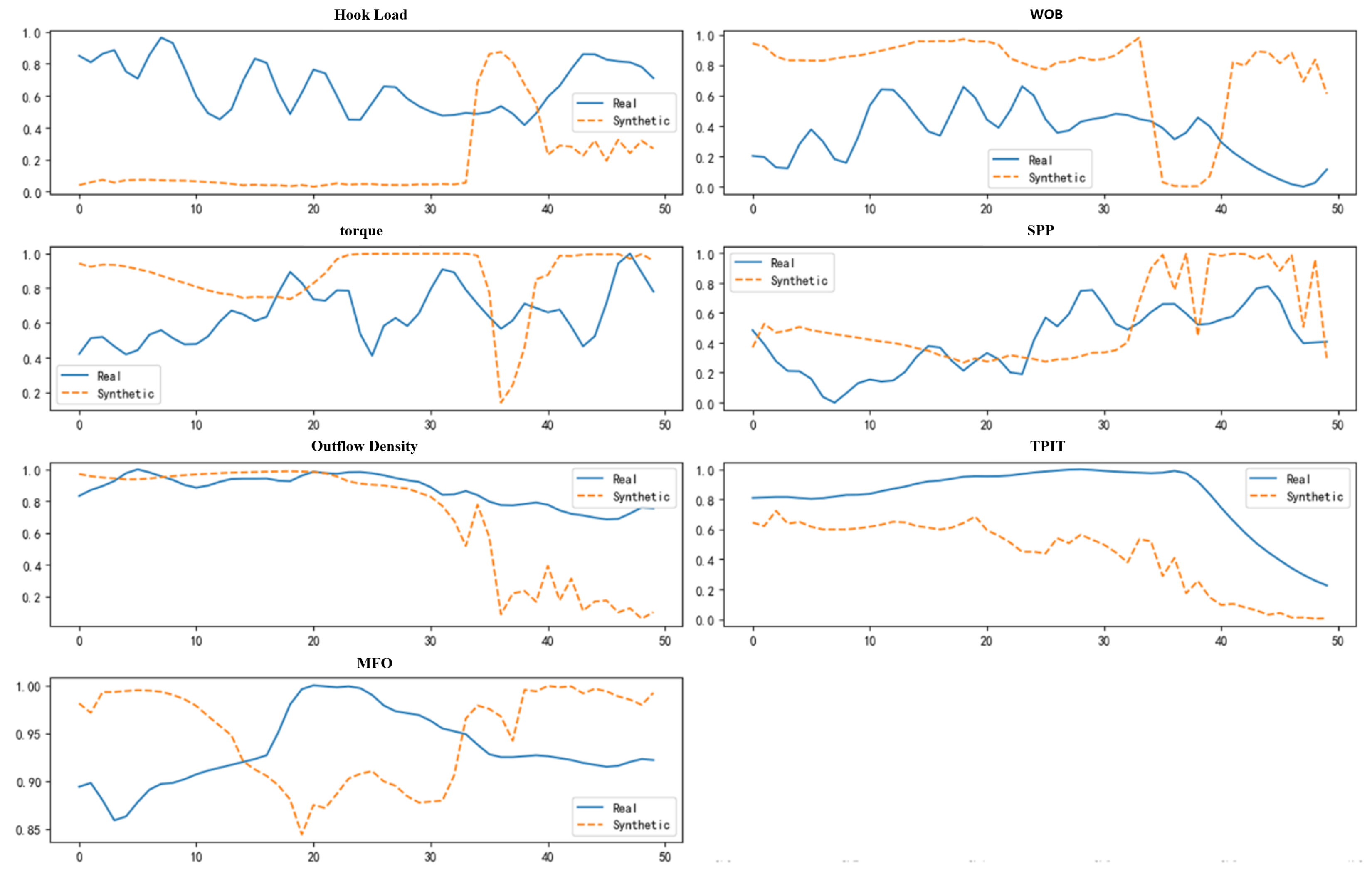
The TimeGAN network constructed in this study generated the lost circulation time series data after 20,000 iterations. The comparison of the generated results with the real samples is shown in Figure 9, where the horizontal axis is the time step and the vertical axis is the normalized value of the feature parameters. While the generated data are numerically distinct from the actual data, they exhibit a certain degree of time series correlation.
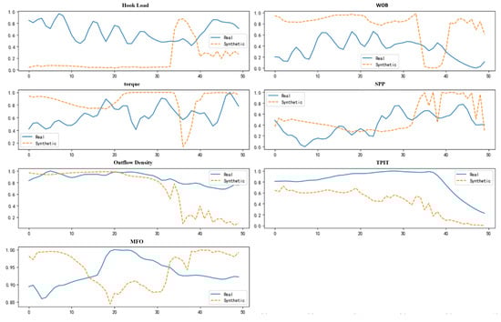
Figure 9.
TimeGAN generation of lost circulation time series data.
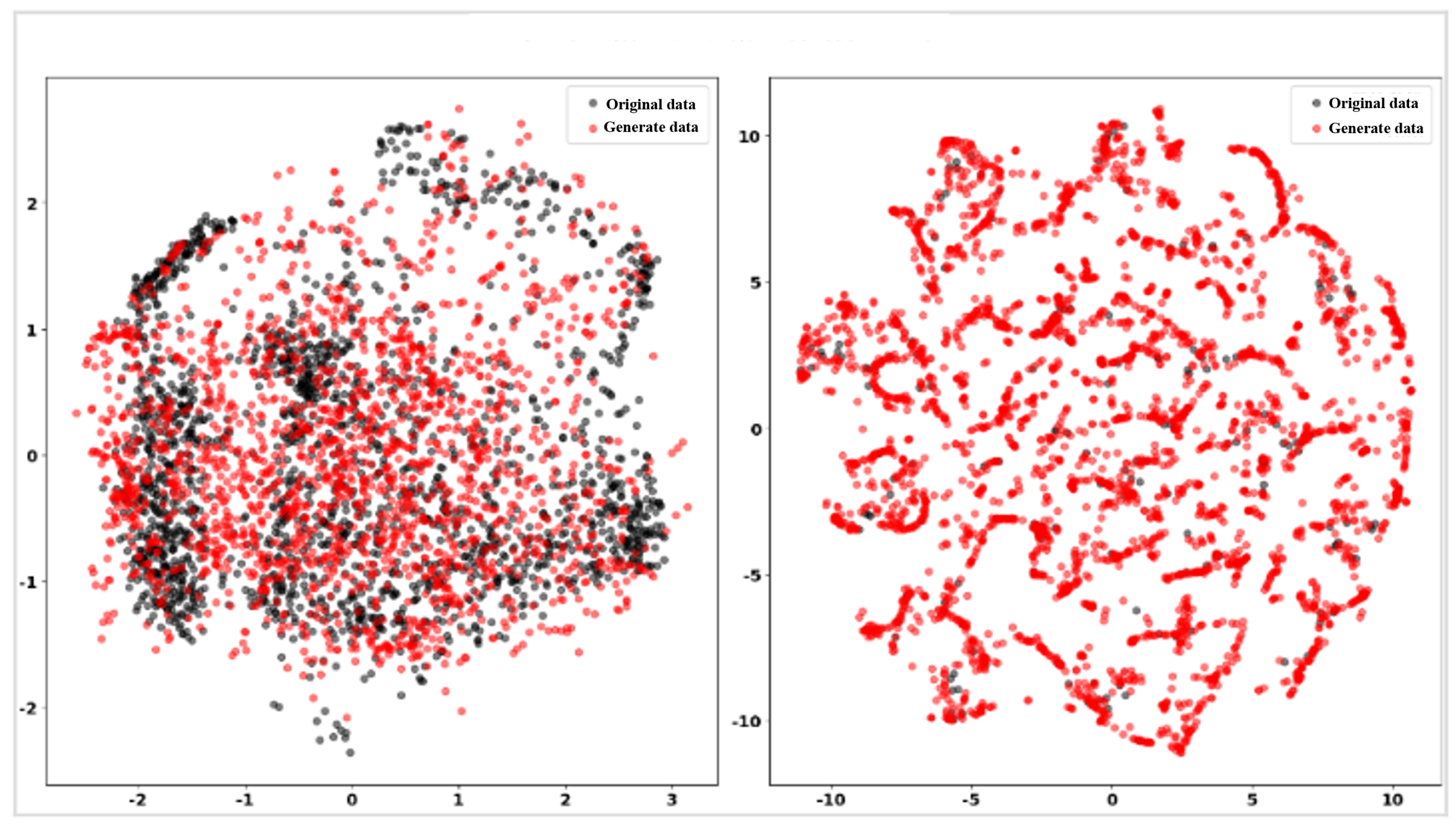
The results are subsequent to PCA and t-SNE dimensionality reduction, which are demonstrated in Figure 10. The proximity of the generated data (red dots) to the original data (black dots) indicates a resemblance between the static and temporal characteristics of the generated data and the real data. As demonstrated in the figure, irrespective of the dimensionality reduction outcomes of PCA or t-SNE, the generated data are distributed in proximity to the hotspot region of the original data and are equally sparse in the sparse area of the original data. This suggests that the TimeGAN-generated lost circulation temporal data features are more aligned with the real data.

Figure 10.
PCA and T-SNE visualization results of generated data versus raw data.
4. Model Construction
4.1. Evaluation Metrics
A significant aspect of employing machine learning methodologies to address engineering challenges is the assessment of the algorithmic models’ efficacy. This study uses five evaluation metrics (i.e., accuracy, precision, recall, missing alarm, and false alarm [15]) to evaluate the performance of diverse models in identifying lost circulation risk [16]. The calculation formulae for each evaluation index are delineated in Table 2 and the subsequent equations.
Table 2.
True result vs. forecast result.
TP is defined as the number of samples that are correctly classified as positive by the model; FN is defined as the number of samples that are incorrectly classified as negative by the model; FP is defined as the number of samples that are incorrectly classified as positive by the model; and TN is defined as the number of samples that are correctly classified as negative by the model.
In a classification model, accuracy represents the proportion of correctly classified samples to the total number of samples. Precision represents the proportion of true positive samples among all samples predicted as positive, indicating the model’s ability to avoid false positive predictions. Recall, specifically for positive cases, is the proportion of true positive samples correctly identified out of all actual positive samples. Missing alarm refers to the fraction of actual lost circulation samples that are incorrectly classified as non-lost circulation, representing missed detections. Conversely, false alarm denotes the fraction of non-lost circulation samples that are incorrectly classified as lost circulation, indicating misclassifications among predicted positive samples.
4.2. Parameter Setting
This study decides to extract the effective time period data after the occurrence of each lost circulation case and the normal data of the same duration before the occurrence as the effective modeling dataset for that lost circulation case. Through the above method, this study ultimately obtained a comprehensive logging time series dataset of nearly 60 effective lost circulation cases, totaling 12,000 data entries, with the training set proportion set at 80% and the test set proportion set at 20%.
To test the effectiveness of the TimeGAN model in generating lost circulation time series data, this study used the lost circulation time period data from the lost circulation logging time series dataset constructed in Section 3.3 as the training data. In order to meet the input requirements of the TimeGAN model, firstly, the sliding window method is used to construct the lost circulation time period data into time series samples with fixed window intervals, and the normalization process is carried out.
4.3. Hyperparameter Configuration
In the context of training a model of this nature, two primary types of hyperparameters demand attention: training hyperparameters and structural hyperparameters. The former primarily governs the model’s training process, while the latter determines its structural design.
In the experiment, the native TimeGAN network in the data-synthetic library based on the Python language is utilized to construct the data expansion generation model, and the primary parameter settings of the model are exhibited in Table 3.
Table 3.
TimeGAN parameter settings.
4.4. Hybrid Loss Function Design
In order to enhance the performance of the lost circulation detection model, a hybrid loss function is designed in this study to combine multiple loss objectives to balance the prediction accuracy and feature selection capability while effectively suppressing the overfitting phenomenon. The hybrid loss function consists of the mean square error (MSE) of coordinate regression and the cross-entropy loss of confidence to balance the demands of the classification task and the regression task. The hybrid loss function expression is:
: the mean squared error (MSE) loss, which is used to measure the accuracy of the lost circulation feature regression task, is given by:
The true value is denoted by , the model prediction by , and the number of samples by N.
: cross-entropy loss, which is employed to evaluate the confidence of the occurrence of lost circulation in the classification task, is given by:
where denotes the true label and denotes the probability value predicted by the model.
: regularization loss, which is employed to constrain the complexity of the model and enhance the feature selection capability. In this study, L1 regularization is employed, and its formula is:
w is the weight vector of the model and d is the dimension of the model parameters.
, , : hyperparameters, which are used to regulate the importance of each loss term.
In this study, we set = 0.5, = 0.4, and = 0.1 to balance the prediction accuracy and feature sparsity.
5. Results and Discussion
In this section, the optimization effect of different feature enhancement methods on the model is analyzed, as well as the optimization effect of data expansion methods on the model. In addition, the optimization effect of feature enhancement combined with data expansion on the model is undertaken.
5.1. Analysis of Feature Enhancement Effects via Wavelet Transform
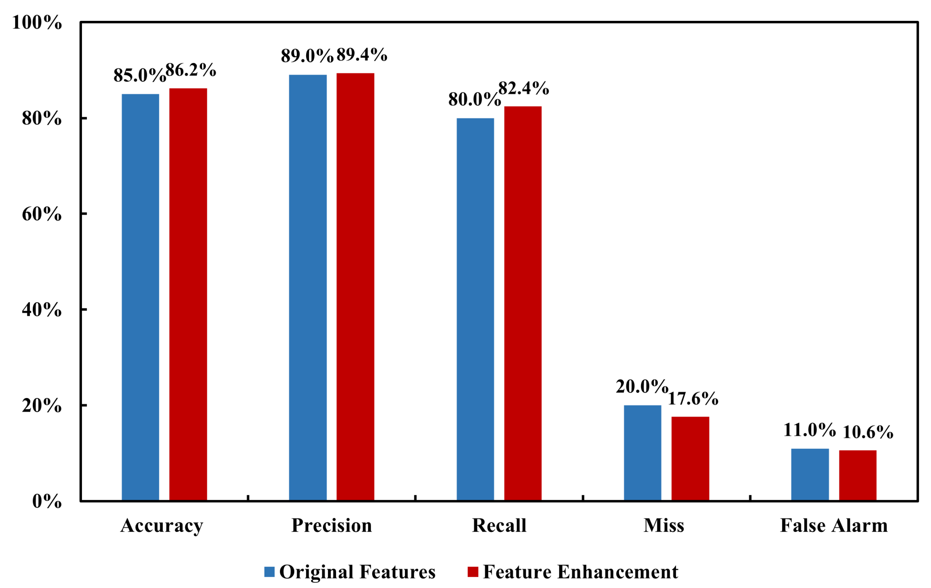
As demonstrated in Figure 11, following the implementation of wavelet transforms for feature enhancement, the evaluation indexes of the model on the test set are optimized in comparison with those prior to feature enhancement. The accuracy rate is increased by 1.2%, the precision rate by 0.4%, the recall rate by 2.4%, and the leakage rate and the false alarm rate are decreased by 2.4% and 0.4%, respectively.

Figure 11.
Evaluation of feature enhancement effects.
5.2. Analysis of Data Augmentation Effectiveness via TimeGAN
As shown in Figure 12, the findings of this study demonstrate that data expansion significantly improves model performance, especially at 1× and 2× expansion. The increase in accuracy is not significant when the expansion is increased from 2× to 4×. The optimum model performance is achieved with 2× expansion. Expansion beyond 2× makes it difficult to achieve a full improvement with the current dataset and significantly increases model training time.
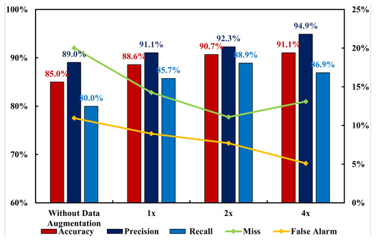
Figure 12.
Comparison of evaluation indicators for test set under different expansion factors.
5.3. Comprehensive Analysis
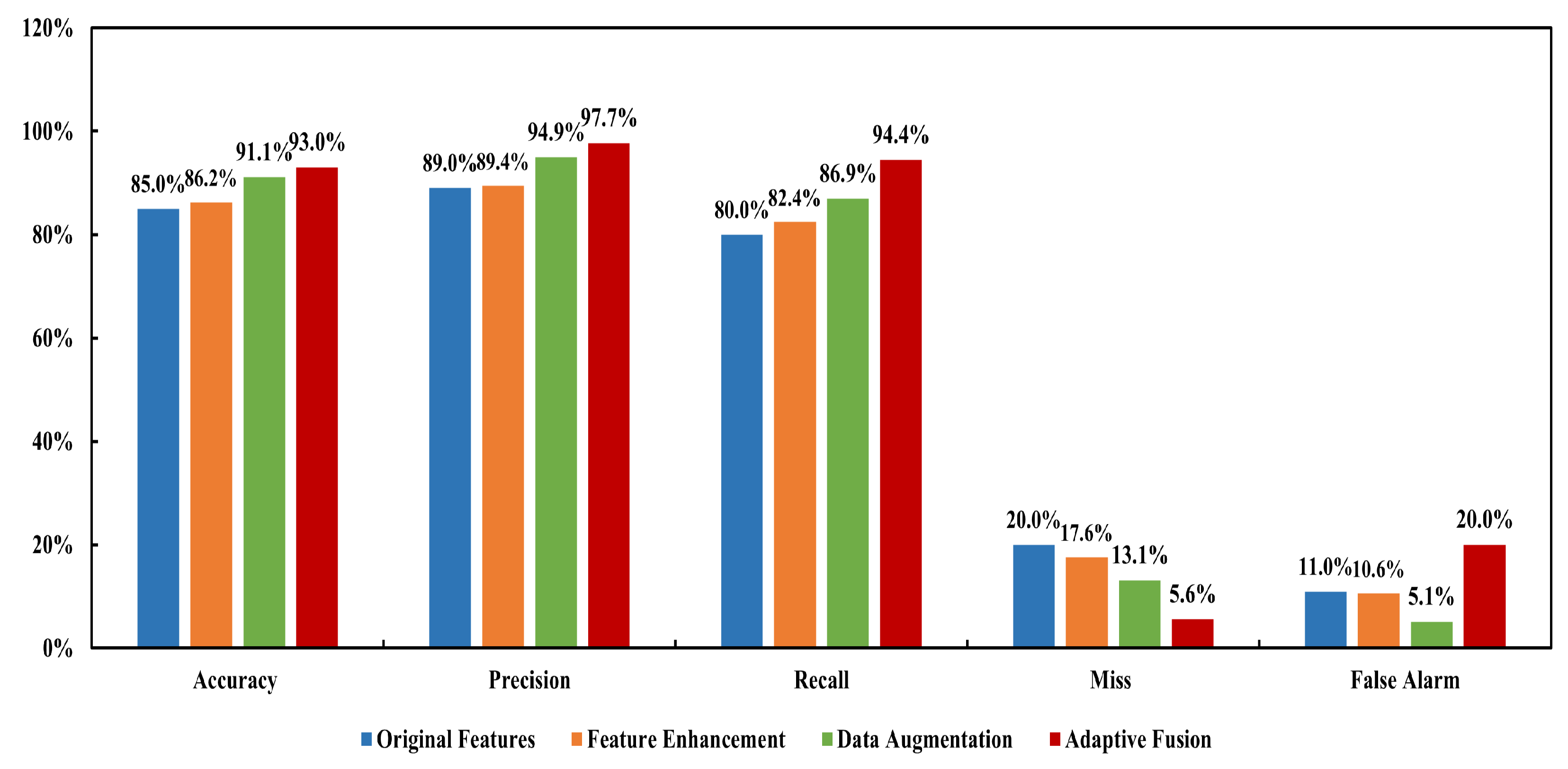
In the context of the original dataset, which exhibits a loss of circulation, both the feature enhancement method and the data expansion method have been shown to enhance the performance of the model. However, it has been demonstrated that the data expansion method exerts a more substantial influence on the model’s performance than the feature enhancement method. In this study, the two aforementioned methods are fused with multi-scale features, and the effect of multi-scale feature fusion optimization on model performance is compared with that of individual optimization, as shown in Figure 13. The multi-scale feature fusion optimization demonstrated superior performance compared to individual optimization, achieving an accuracy of 93.8%, a precision of 95.1%, and a recall of 92.2%. Furthermore, the missing alarm rate and false alarm rate were reduced to 7.6% and 4.8%, respectively.
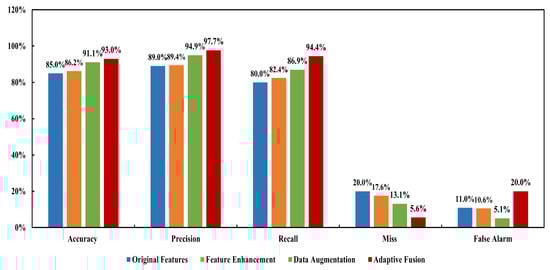
Figure 13.
Comprehensive optimisation effect analysis.
Following the multi-scale feature fusion, the accuracy and precision of the model have been evidently enhanced compared with the unoptimized tandem model. The model demonstrated significant performance improvements across multiple metrics: accuracy increased by 8.8%, precision improved by 6.1%, and recall showed a notable enhancement of 12.2%. Additionally, both the missing alarm rate and false alarm rate decreased substantially, with reductions of 12.4% and 6.2%, respectively.
As illustrated in Figure 14, the multi-scale feature fusion model outperforms the baseline models (Random Forest, XGBoost, LSTM, and BiLSTM) across all metrics, including accuracy, recall, precision, missing alarm rate, and false alarm rate, which highlights its superior feature integration ability.
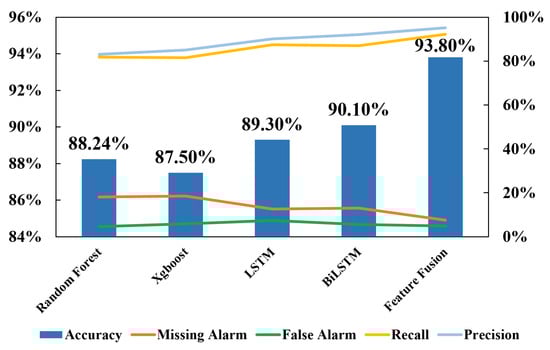
Figure 14.
Comparison of the effect of different models.
6. Conclusions
To assess the optimization effect, the lost circulation time series feature enhancement method and time series data expansion method, in conjunction with the multi-scale feature fusion method, which optimizes the model’s stability and generalization ability, are employed.
The fusion of feature wavelet transform and genetic programming has been shown to extract effective enhancement features from both deep feature mapping and feature deformation perspectives, thereby significantly improving the diagnostic performance of the model. When the enhanced features of both are used as inputs, the model performs optimally with 87.5% accuracy and 83.4% recall.
Furthermore, the TimeGAN network has been demonstrated to achieve multidimensional expansion of lost circulation time series data, with the generated data exhibiting a distribution similar to that of the original data. This data expansion has been shown to improve model performance and substantially reduce the occurrence of overfitting.
With an increase in the expansion multiplier, the model’s performance on the test set gradually enhances. When the expansion multiplier is set to 2, the model achieves a balance between performance enhancement and training time, with the accuracy of the test set reaching 90.7%, the missing alarm rate at 11.1%, and the false alarm rate at 7.7%.
The effect of the multi-scale fusion feature method is better than that of single optimization. Compared with the non-optimized model, the final optimization results show that the accuracy rate is increased by 8.8%, the precision rate is increased by 6.1%, the recall rate is increased by 12.2%, and the missing alarm rate and false alarm rate are decreased by 12.4% and 6.2%, respectively.
Although the data generated by TimeGAN resemble the original data distribution, their diversity is constrained by the training sample size. If the original data contain class imbalance or noise interference, they may introduce biases into the generated data, compromising model robustness. The multi-scale decomposition of wavelet transform and the adversarial training mechanism of TimeGAN increase computational overhead. For instance, while the model adopts batch processing () and a lightweight network structure (), enabling millisecond-level inference time per instance, TimeGAN requires simultaneous training of the generator, discriminator, and embedding network. Additionally, the real-time feature extraction via wavelet transformation demands extra computational resources. High-performance computing support remains essential when processing large-scale real-time drilling data.
Author Contributions
Conceptualization, Y.S.; Methodology, Y.S., J.W. and Z.Z. (Ziyue Zhang); Software, Z.Z. (Ziyue Zhang); Validation, J.W.; Formal analysis, F.F.; Investigation, J.W.; Data curation, Y.S. and J.W.; Writing—original draft, Y.S.; Writing—review & editing, F.F.; Supervision, Z.Z. (Zhaopeng Zhu); Project administration, Z.Z. (Zhaopeng Zhu); Funding acquisition, Z.Z. (Zhaopeng Zhu). All authors have read and agreed to the published version of the manuscript.
Funding
This research was funded by National Natural Science Foundation of China grant number 52204020.
Data Availability Statement
The data presented in this study are available on request from the corresponding author.
Conflicts of Interest
Authors Yuan Sun, Jiangtao Wang and Fei Fan were employed by the China France Bohai Geoservices Co., Ltd. The remaining authors declare that the research was conducted in the absence of any commercial or financial relationships that could be construed as a potential conflict of interest.
Abbreviations
The following abbreviations are used in this manuscript:
| BP | Back Propagation |
| GAN | Generative Adversarial Network |
| SPP | Standpipe Pressure |
| TPIT | Total Pool Volume |
| MFO | Outlet Flow Rate |
| MFI | Inlet Flow Rate |
| GRU | Gated Recurrent Unit |
| WT | Wavelet Transform |
| TimeGAN | Time Series Generative Adversarial Network |
| PCA | Principal Component Analysis |
| t-SNE | t-Distributed Stochastic Neighbor Embedding |
| TP | True Positive |
| FN | False Negative |
| FP | False Positive |
| TN | True Negative |
References
- Elmousalami, H.; Sakr, I. Artificial intelligence for drilling lost circulation: A systematic literature review. Geoenergy Sci. Eng. 2024, 239, 212837. [Google Scholar] [CrossRef]
- Albattat, R.; AlSinan, M.; Kwak, H.; Hoteit, H. Modeling lost-circulation in natural fractures using semi-analytical solutions and type-curves. J. Pet. Sci. Eng. 2022, 216, 110770. [Google Scholar] [CrossRef]
- Liu, Z.; Ma, Q.; Shi, X.; Chen, Q.; Han, Z.; Cai, B.; Liu, Y. A dynamic quantitative risk assessment method for drilling well control by integrating multi types of risk factors. Process Saf. Environ. Prot. 2022, 167, 162–172. [Google Scholar] [CrossRef]
- Saifulizan, S.S.B.H.; Busahmin, B.; Prasad, D.M.R.; Elmabrouk, S. Evaluation of different well control methods concentrating on the application of conventional drilling technique. ARPN J. Eng. Appl. Sci. 2023, 18, 1851–1857. [Google Scholar]
- Menghan, S. Research on Real-Time Early Warning Method for Drilling Kick. Master’s Thesis, Southwest Petroleum University, Chengdu, China, 2016. [Google Scholar]
- Al-Hameedi, A.T.T.; Alkinani, H.H.; Dunn-Norman, S.; Flori, R.E.; Hilgedick, S.A.; Amer, A.S.; Alsaba, M. Mud Loss Estimation Using Machine Learning Approach. J. Pet. Explor. Prod. Technol. 2019, 9, 1339–1354. [Google Scholar] [CrossRef]
- Yan, Y.; Mubai, D.; Hao, H. Research on Drilling Risk Early Warning Technology Based on Trendline Method. Drill. Prod. Technol. 2023, 46, 170–174. [Google Scholar]
- Zhuo, Z.; Zhichao, S.; Bo, C.; Pengfei, H.; Changfang, J.; Tong, X. Research on Lost Circulation Early Warning Model Based on XGBoost Algorithm. Petrochem. Appl. 2023, 42, 112–115. [Google Scholar]
- Weifeng, S.; Saisai, B.; Dezhi, Z.; Weihua, L.; Kai, L.; Yongshou, D. Intelligent Monitoring Method for Micro-Loss of Drilling Fluid Based on DCC-LSTM. Nat. Gas Ind. 2023, 43, 141–148. [Google Scholar]
- Grossmann, A.; Morlet, J. Decomposition of Hardy Functions into Square Integrable Wavelets of Constant Shape. SIAM J. Math. Anal. 1984, 15, 723–736. [Google Scholar] [CrossRef]
- Yoon, J.; Jarrett, D.; van der Schaar, M. Time-series generative adversarial networks. In Proceedings of the 33rd International Conference on Neural Information Processing Systems, Vancouver, BC, Canada, 8–14 December 2019; Curran Associates Inc.: Red Hook, NY, USA, 2019; p. 11. [Google Scholar]
- Hongyu, Z.; Zhiwen, Z.; Maoguo, G.; Yue, W.; Zhou, Y.; Yuzhou, L.; Yang, Z. Drone Detection in Radar Echo Based on Data Augmentation and Feature Enhancement. Shanghai Aerosp. 2023, 40, 61–69. [Google Scholar] [CrossRef]
- Zhou, M.; Kangning, D.; Dinghui, W. Small Sample Fault Diagnosis of Bearings Based on Multi-Scale Cross-Feature Fusion Siamese Network. Control Eng. 2024, 1–8. [Google Scholar] [CrossRef]
- Li, S.; Hao, Q.; Kang, X.; Benediktsson, J.A. Gaussian Pyramid Based Multiscale Feature Fusion for Hyperspectral Image Classification. IEEE J. Sel. Top. Appl. Earth Obs. Remote Sens. 2018, 11, 3312–3324. [Google Scholar] [CrossRef]
- Weifeng, S.; Kai, L.; Dezhi, Z.; Weihua, L.; Liming, X.; Yongshou, D. Overflow and Well Leakage Monitoring Method Combining Drilling Conditions and Bi-GRU. Pet. Drill. Tech. 2023, 51, 37–44. [Google Scholar]
- Wu, L.; Wang, X.; Zhang, Z.; Zhu, G.; Zhang, Q.; Dong, P.; Wang, J.; Zhu, Z. Intelligent Monitoring Model for Lost Circulation Based on Unsupervised Time Series Autoencoder. Processes 2024, 12, 1297. [Google Scholar] [CrossRef]


Disclaimer/Publisher’s Note: The statements, opinions and data contained in all publications are solely those of the individual author(s) and contributor(s) and not of MDPI and/or the editor(s). MDPI and/or the editor(s) disclaim responsibility for any injury to people or property resulting from any ideas, methods, instructions or products referred to in the content. |
© 2025 by the authors. Licensee MDPI, Basel, Switzerland. This article is an open access article distributed under the terms and conditions of the Creative Commons Attribution (CC BY) license (https://creativecommons.org/licenses/by/4.0/).