1. Introduction
The 3D braided composites have a specific geometric position relationship between braided fibers and matrix by pre-setting the braiding mode of fibers, so as to ensure that the materials have excellent mechanical properties in a specific direction and show good performance with designable characteristics. In recent years, with the improvement in braiding technology and the reduction in manufacturing cost, 3D braided composites have been widely used in aviation, aerospace, navigation, transportation, medical care, sports, and civil engineering [
1,
2,
3].
In order to obtain 3D braided composites with different structures, the braiding methods can be divided into rectangular braiding and circular braiding according to the structural differences of preforms. In the aspect of reasonable construction of rectangular braided material model, Tian et al. proposed a diversity-oriented particle swarm optimization (DPSO-MLS) with multilevel learning strategy, which can be used to optimize the composite structure [
4]. Zhang and Xu, based on the analysis of braiding laws of 3D five-directional and all five-directional braided composites, divided the studied materials into three kinds of cell models: inner, surface, and corner. By introducing reasonable boundary conditions, they predicted the effective stiffness characteristics of the materials, and compared the detailed mechanical properties of the three cell models. In addition, the effects of braiding angle and fiber volume fraction on the elastic properties of the composites were also analyzed [
5,
6,
7]. Inspired by the slub fiber structure, Wang et al. designed and prepared a new type of three-dimensional six-way braided composite pipe [
8].
In the aspect of mechanical properties of rectangular braiding, Ji et al. [
9] analyzed the geometric model of composite materials with the help of finite element analysis software Abaqus 15.0, and obtained the elastic modulus, shear modulus, and Poisson’s ratio of composite materials corresponding to different braiding angles. The influence of fiber volume fraction on the elastic properties of composite element is also studied, and the bending properties of braided composite material are evaluated by the multi-scale model in finite element analysis. The experimental results show that the predicted results are basically consistent with the experimental results. In order to study the progressive damage behavior and strength characteristics under uniaxial tension, Kang et al. established a finite element and progressive damage analysis model, and compared the finite element analysis results with experimental data [
10]. Sun et al. [
11] studied the effects of fiber fracture defects and corrugation defects on compressive fatigue behavior and damage evolution process of three-dimensional multiaxial braided composites.
The above research focuses on rectangular braiding. Compared with rectangular braiding, the micro-geometric structure of circular braiding is more complicated than that of rectangular preform, and it is more difficult to analyze its structure and mechanical properties theoretically [
12,
13,
14]. Zhao and Li et al. [
15,
16] selected a micro-geometric cell, and found that the curvature of annular pipe has great influence on braided composites. The elastic modulus of braided composites of annular pipe was predicted by mathematical models, and the predicted results were found to be reasonable by comparing with the literature data. Shen [
17] tested the compression and torsion mechanical properties of 3D, 4D, and 5D braided tubular members through experiments, and found that the compression properties of 5D materials were greatly improved compared with 4D materials, but the shear modulus was not significantly improved. Comparing the experimental data with the prediction data of FGM model, it was concluded that the prediction results of FGM simulation were lower. Zhang [
18] applied braided composite materials to two-stage gear transmission system, realizing the design goal of lightweight gear transmission system.
As can be seen from the above literature, most of the research on braided composites is focused on rectangular braiding and circular braiding, but there are few research papers on the prediction of mechanical properties of 3D five-way circular braiding. Because of the anisotropy of mechanical properties of 3D five-way circular braided composites, the research in this paper provides the possibility for the special performance requirements of materials, such as the application of composites subjected to radial force, which is of great value.
The paper is divided into seven sections. In
Section 2, the motion law of 3D five-directional circular braiding fiber is analyzed, and the composite material is divided into three microscopic cells. In
Section 3, the formulas for calculating the overall stiffness matrix and fiber volume content of 3D five-directional circular braided composites are derived, and the mechanical properties of the composites can be obtained by inverting the overall stiffness matrix of the composites. In
Section 4, the prediction model derived in this paper is used to further numerically analyze the mechanical properties of cells. In
Section 5, there is numerical analysis of the influence of braiding parameters on the mechanical properties of cells. In
Section 6, on the basis of the above analysis, the parametric study is completed. In
Section 7, we state the main conclusions. In this paper, the numerical prediction model for mechanical properties of 3D five-directional circular braided composites fully considers the braiding parameters such as cell inner diameter, cell outer diameter, cell height, and knuckle length, and can quantitatively analyze the influence of different braiding parameters on the mechanical properties of composites.
3. The Solving the Stress Transformation Matrix of Circular Braiding
In the process of 3D five-directional circular braiding, the fiber movement is carried out in the
polar coordinate system in
Figure 3, and the braiding angle is calculated under the
global coordinate rectangular system in
Figure 3. The polar coordinate system
is located on the inclined section of MNQ, and the
axis is parallel to the outer normal of plane MNQ, and the coordinate axis
and
are on plane MNQ.
In
Figure 3, when M, N, and Q points approach infinitely to the origin
of polar coordinate system
along the opposite directions of
,
, and
axes, respectively, the stress on the annular hexahedron element shown in
Figure 3 is approximately equal to the stress on the inclined section MNQ.
Assuming that the force on the circular-shaped micro hexahedron element is not considered, the area of the inclined section will be projected on the three coordinate axes of the polar coordinate system , and the relationship between the areas is obtained: , , .
Assume that the total stress on the inclined section MNQ is F, and the components of F along the coordinate axis in polar coordinate system are expressed by, and respectively.
According to the equilibrium conditions
,
, and
, and in the annular hexahedron element in
Figure 3, we can obtain:
The moment balance condition
,
, and
are applied to the center of gravity coordinate axis of the annular hexahedron in
Figure 3, we can obtain
,
and
.
The force in Formula (1) is decomposed along the three coordinate axes of polar coordinate system
, and according to the angle relationship shown in
Figure 3, the stress
,
, and
on the inclined section MNQ is:
In
Figure 4, the
axis is parallel to the outer normal of the plane
,
is the angle between the axes
and
; according to the angle relationship in
Figure 4, we can obtain
.
Let the area of inclined section
be
, and project
on three coordinate axes plane of polar coordinate system
, and obtain the relationship between areas
,
,
. According to the equilibrium conditions in the annular hexahedron unit in
Figure 4:
The force in Formula (3) is decomposed along three coordinate axes of polar coordinate system
, according to the angular relationship shown in
Figure 4, the stresses
,
, and
on the inclined section
are obtained as follows:
In the same way,
can be obtained when the inclined section is parallel to the outer normal of the
axis. By using Formulas (2) and (4), the relationship matrix of stress components on the inclined section of the annular hexahedron element in polar coordinate system can be obtained as follows:
In Formula (5),
is the spatial transformation matrix of circular braiding stress,
is a 6 × 6 matrix, which is given in
Appendix A.
4. The Equivalent Stiffness Matrix of Cells
4.1. Solving the Equivalent Stiffness Matrix of Internal Cells
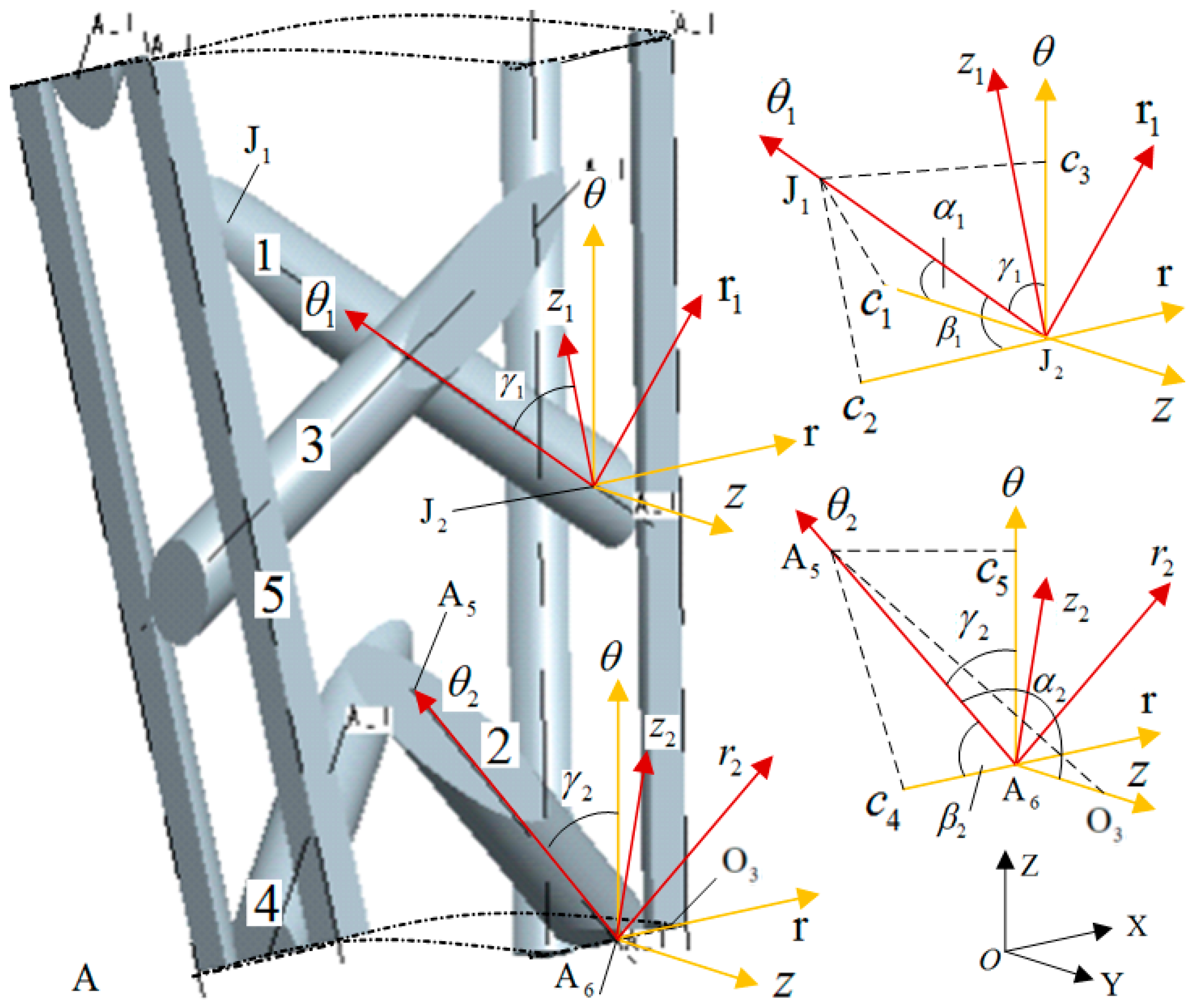
Figure 5 shows the fiber angle relationship in the inner cell A, and the coordinates of
and
points in the cylindrical coordinate system
in
Figure 5 are:
Therefore, the coordinates of the
and
points in the
rectangular coordinate system are:
According to the relationship between cylindrical coordinate system
and rectangular coordinate system
, in
Figure 5, the distance between
and
points in rectangular coordinate system
is:
The distance between the
and
points in the cylindrical-coordinate system
is:
Therefore, the coordinates of the
and
points in rectangular coordinate system
are:
Therefore, according to the positional relationship between the two coordinate systems, in
Figure 5, the distance between the
and
points in the
rectangular coordinate system is
, the distance between
and
is [
21]:
According to the positional relationship shown in
Figure 5, the formulas for calculating the angle between the
axis and the three coordinate axes
on fiber 1 in inner cell A can be obtained:
In Formula (12), the angle between the inner braiding fiber and the braiding direction is defined as the inner braiding angle, and is the inner braiding angle of the outer layer fiber of inner cell A.
In the same way, according to the positional relationship shown in
Figure 5, the formulas for calculating the angle between the
axis on fiber 2 in inner cell A and the three coordinate axes of
can be obtained:
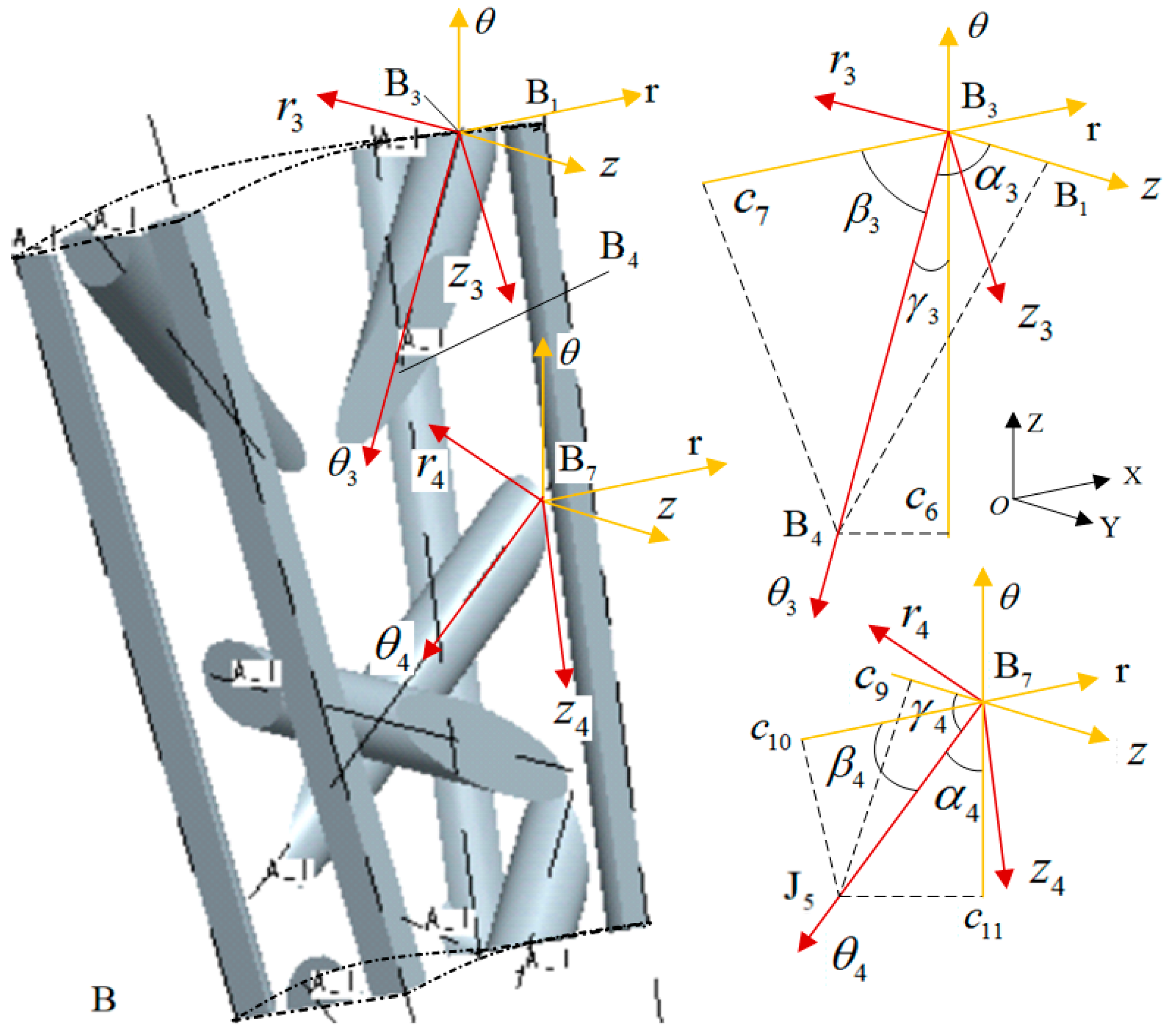
In the same way, according to the positional relationship shown in
Figure 6, the formulas for calculating the angle between
axis and
three coordinate axes on fiber 1 in inner cell B can be obtained:
In the same way, the formulas for calculating the angle between
axis and
three coordinate axes on fiber 2 in inner cell B can be obtained:
In Formulas (14) and (15),
There are five kinds of fibers with different orientations in inner cell A. According to the positional relationship shown in
Figure 5, the angles between the five kinds of fibers in inner cell A and the coordinate axis are shown in
Table 1.
In the same way, there are five kinds of fibers with different directions in inner cell B. According to the positional relationship shown in
Figure 6, the angles between the five kinds of fibers in inner cell B and the coordinate axis can be obtained, as shown in
Table 2.
Because of the symmetry of inner cell structure, the angle between fiber and coordinate axis in inner cell D is the same as that in inner cell A, and the angle between fiber and coordinate axis in inner cell C is the same as that in inner cell B.
Therefore, the stiffness matrix of inner cell A is:
In Formula (16),
is the fiber volume ratio of fiber
in inner cell A to inner cell A,
is the stress transformation matrix of fiber
in inner cell A, and the angles in
Table 1 are brought into Formula (5). According to Formulas (13) and (15), the stress transformation matrix
of inner cell A can be obtained.
is the stiffness matrix of fiber in local coordinates [
16,
17].
In Formula (17),
, in the same way, the stiffness matrices
,
, and
of internal cells
B,
C, and
D can be obtained.
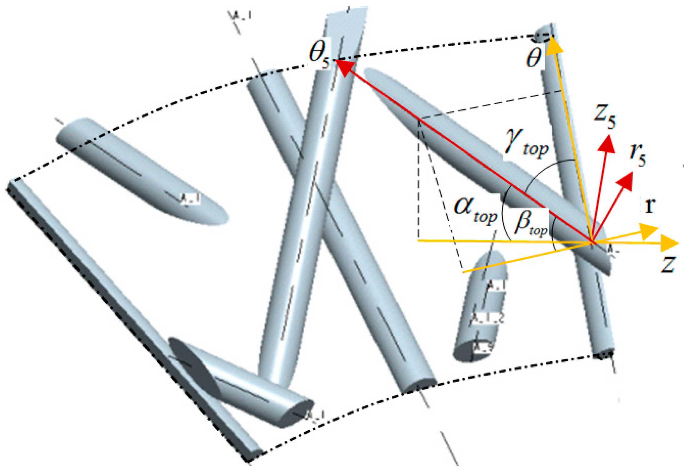
4.2. Solving the Equivalent Stiffness Matrix of Upper Surface Cells
Figure 7 shows the fiber angle relationship in the upper surface cell. Similarly, according to the position relationship shown in
Figure 7, the calculation formulas of the angles between
axis and
axis on the fiber in the upper surface cell can be obtained:
In Formula (19), .
In the same way, the equivalent stiffness matrix
of the upper surface cell is:
In Formula (20), , .
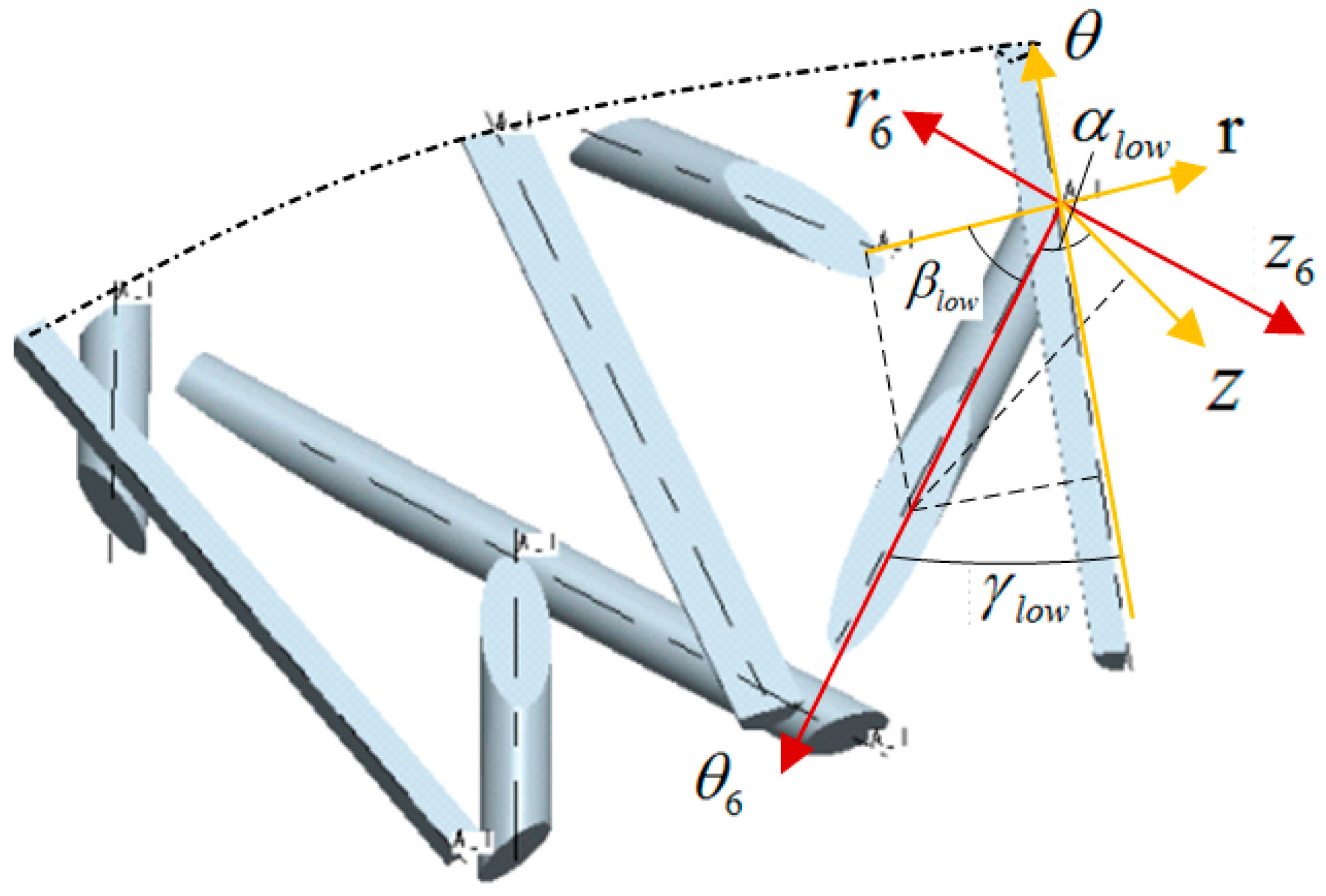
4.3. Solving the Equivalent Stiffness Matrix of Lower Surface Cells
Figure 8 shows the angle relationship of fibers in the lower surface cells. Similarly, according to the position relationship shown in
Figure 8, the calculation formulas of the angle between
axis and
axis on the fiber in the lower surface cells can be obtained:
In Formula (21), .
In the same way, the equivalent stiffness matrix
of the lower surface cell is:
In Formula (22), , .
Therefore, the overall stiffness matrix of all fibers of the whole annular braided composite material is:
In Formula (23), , , .
The overall stiffness matrix of that 3D and five-direction annular braided composite material considering the matrix is as follows:
In Formula (24), is the fiber volume fraction, is matrix of matrix stiffness.
The calculation formulas of fiber volume fraction is as follows [
21]:
In Formula (25),
is the total volume of internal cells,
is the volume of fibers in the inner cell,
is the cross-sectional area of braided fiber bundle, and the cross-sectional shape of braided fiber is oval,
, the half of major axis of ellipse is
, the half of the minor axis of ellipse is
.
is the cross-sectional area of the axial fiber, the cross-sectional shape of the axial fiber is square
, the side length is
,
is the cross-sectional dimension coefficient of axial fiber [
17,
18,
21].
Table 3 gives the mechanical property parameters of fibers and matrix in carbon fiber braided composites. Because the 3D five-directional circular transverse braided materials approximately meet the conditions of transverse isotropy in a certain radial range in the plane perpendicular to the Z axis, the elastic modulus satisfies:
, the shear modulus meets the following requirements:
, and Poisson’s ratio meets the following requirements:
. Because the matrix is an isotropic material, the shear modulus of the matrix meets the following requirements:
.
According to the parameters of composite fibers and matrix in
Table 3, the mechanical parameters of fiber bundles in composite materials in all directions can be calculated by using Chamis mechanical formulas shown in Formula (26) [
21,
22].
In Formula (26),
is the elastic modulus of fiber bundle in
direction,
is the filling coefficient of matrix and fiber in fiber bundle,
is the elastic modulus of matrix,
is the elastic modulus of fiber in
direction,
is the shear modulus of fiber bundle in
planes,
is the shear modulus of fiber in
planes,
is Poisson’s ratio of fiber bundle in
planes,
is Poisson’s ratio of fiber in
direction [
18,
21].
5. Numerical Analysis of the Influence of Braiding Parameters on the Mechanical Properties of Cells
The matrix parameters in
Table 3 and the parameters of fiber bundles obtained by Formula (26) are brought into Formula (24), and the overall stiffness matrix of 3D five-directional annular braided composites can be obtained. By inverting the overall stiffness matrix, the engineering elastic constant of 3D five-directional annular braided composites can be obtained as shown in Formula (27).
In Formula (27), is the overall flexibility matrix of composite materials, is the elastic modulus of the composite material in the direction, is the shear modulus of the composite in the planes, is Poisson’s ratio of composite materials in planes.
The length of braiding knuckles h = 2 mm, inner cell diameter = 7 mm, M and N are radial and axial braided fibers M = N = 80, respectively. The height of internal cells = 0.5 mm, the filling factor .
The numerical results calculated by Formula (27) are compared with the experimental results in reference [
17], and the results are shown in
Table 4. It is found that the relative error between the numerical prediction model deduced in this paper and the experimental results is 6.6%.
In order to further analyze the influence of braiding parameters on the mechanical properties of 3D five-directional circular braided composites, the mathematical model described in this paper is used to numerically analyze the influence of braiding parameters on the mechanical properties of cells.
The relationship between that braiding angle
γ and the knuckle length
h of the 3D circular braiding material is shown in
Figure 9, in which the cell inner diameter
, the height of the inner cell
, the number of radial and axial braiding fibers
. It can be seen from
Figure 9 that the braiding angles of the four internal cells are relatively close, that is,
. With the increase in the length h of the knuckle, the braiding angles of each cell decrease, and the braiding angles of the four inner cells decrease the most; when that knuckle length increases from 1 mm to 3 mm, the braiding angle of the four inner cells is reduced by 38%~46%. With the increase in the length h of the knuckle, the braiding angle of the upper and lower surfaces decreases slightly, that is,
; when that knuckle length increases from 1 mm to 3 mm, the braiding angle of the upper and lower surfaces is reduced by 7.1%.
Figure 10 shows the influence curve of cell height
and knuckle length h on fiber volume content
and transverse elastic modulus
. It can be seen from
Figure 10 that with the increase in knuckle length h and cell height
, the fiber volume content
of 3D five-directional annular braided composites decreases; when that knuckle length increase from 1 mm to 10 mm, the fiber volume content is reduced by 57.1%. With the increase in knuckle length h, the transverse elastic modulus
first increases and then decreases slowly, and with the increase in cell height
, the transverse elastic modulus
decreases. This is mainly because fiber volume content decreases due to the increase in knuckle length and cell height, and the number of carbon fibers per unit volume decreases, which, in turn, leads to a decrease in transverse elastic modulus.
Figure 11 shows the influence curve of cell height
and knuckle length
on fiber volume content
and longitudinal elastic modulus
. It can be seen from
Figure 11 that with the increase in knuckle length
and cell height
, the fiber volume content
of 3D five-directional annular braided composites decreases. The longitudinal elastic modulus
increases rapidly when the length of knuckle
, and increases slowly when
. When the knuckle length
, the longitudinal elastic modulus
increases with the increase in the cell height
. When the node length
, the longitudinal elastic modulus decreases with the increase in cell height
. The above results show that the cell height has less influence on longitudinal elastic modulus and more influence on fiber volume content.
It can be seen from
Figure 12 that with the increase in knuckle length
h, the fiber volume content
decreases, and the shear modulus first increases and then decreases. With the increase in cell height
, the fiber volume content and elastic modulus decrease linearly. The above results show that the shear modulus
is greater than the shear modulus
, and this is mainly because the mechanical properties of materials along the braiding direction are the best.
It can be seen from
Figure 13 that with that knuckle length increase from 5 mm to 10 mm, the transverse elastic modulus is reduced by 8.6%; when the filling factor increases from 0.87 to 0.95, the transverse elastic modulus is increased by 7.5%; when the number of braiding fibers increases from 20 to 40, the transverse elastic modulus is increased by 114%.
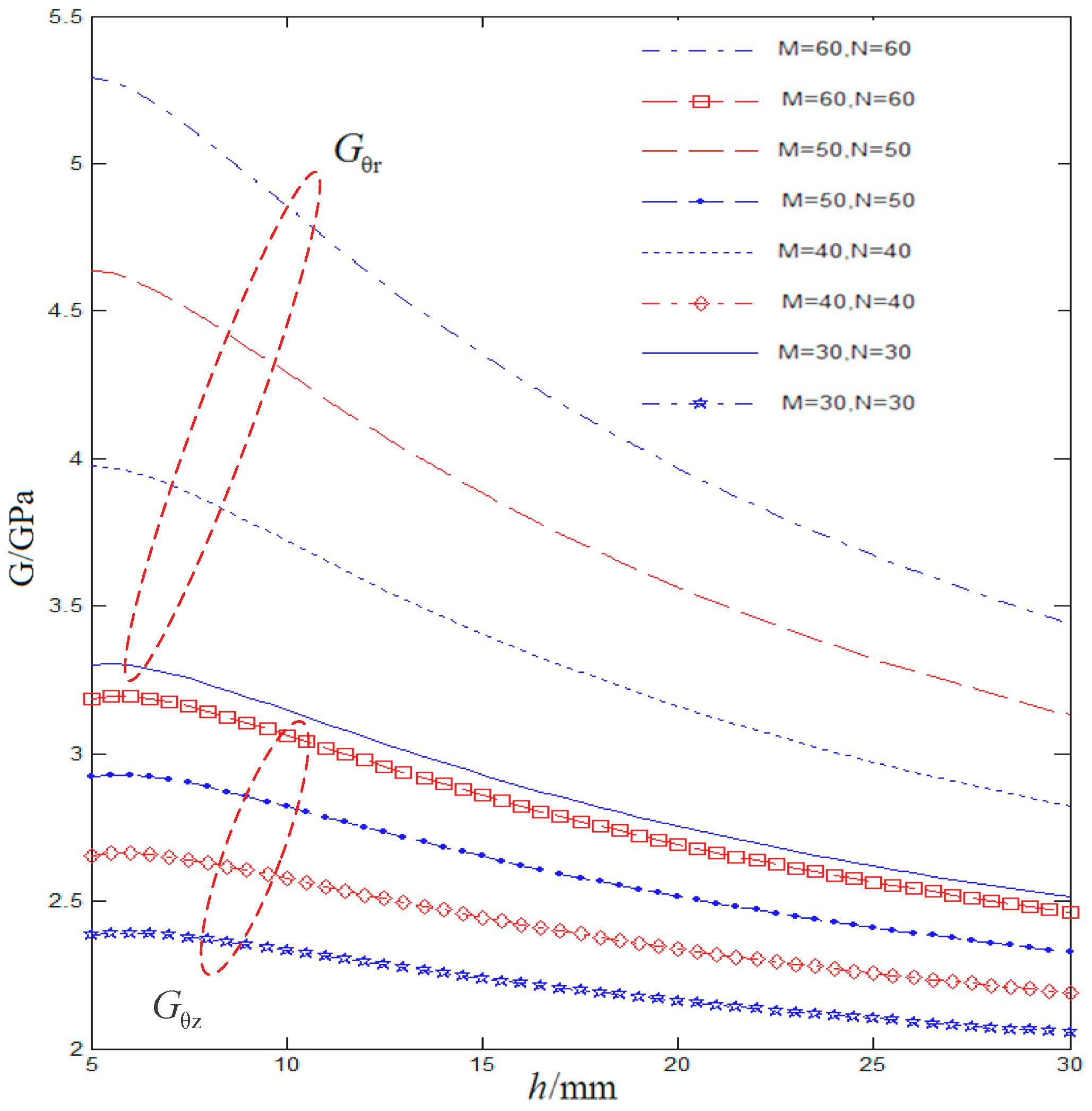
It can be seen from
Figure 14 that with that knuckle length increase from 5 mm to 30 mm, the shear modulus
is reduced by 33%, the shear modulus
is reduced by 31%, and when the number of braiding fibers increases, the shear modulus is increased.


 ,
, 

