Analytical Solutions and Stability Analysis of a Fractional-Order Open-Loop CSTR Model for PMMA Polymerization

Abstract

This study examines the asymptotic stability of a continuous stirred tank reactor (CSTR) used for poly(methyl methacrylate) (PMMA) polymerisation, utilizing nonlinear fractional-order mathematical models. By applying Taylor series and Laplace transform techniques analytically and incorporating real plant data, we focus exclusively on the chemical reaction effects in the kinetic constants, disregarding mass transport phenomena. Our results confirm that fractional derivatives significantly enhance the stability and performance of dynamic models compared to traditional integer-order approaches. Specifically, we analyze the stability of a linearized fractional-order system at steady state, demonstrating that the system maintains asymptotic stability within feasible operational limits. Variations in the fractional order reveal distinct impacts on stability regions and system performance, with optimal values leading to improved monomer conversion, polymer concentration, and weight-average molecular weight. Comparative analyses between fractional- and integer-order models show that fractional-order operators broaden stability regions and enable precise tuning of process variables. These findings underscore the efficiency gains achievable through fractional differential equations in polymerisation reactors, positioning fractional calculus as a powerful tool for optimizing CSTR-based polymer production.

1. Introduction

In polymerisation reactor engineering, maintaining stability in continuous stirred tank reactors (CSTRs) is a critical challenge, especially for processes involving free radical polymerisation, such as the production of polymethyl methacrylate (PMMA). These reactors operate in non-linear dynamics, where the presence of diffusion-controlled effects, including the gel effect, the glass effect, and the cage effect, significantly affects reaction kinetics and reactor stability [1,2]. Ensuring asymptotic stability in these systems is essential for achieving consistent polymer quality and efficient raw material conversion. Traditional integer order mathematical models struggle to capture the complexities of these polymerisation processes, often leading to limited stability regions and reduced predictive accuracy [3].

To address these limitations, fractional differential equations have emerged as a powerful tool for improved mathematical modelling, simulation, and stability analysis of inherently unstable and nonlinear systems [4,5]. The advantage of fractional derivatives lies in their ability to incorporate long-term memory effects, which better describe the history-dependent behaviour of polymerisation kinetics [6,7]. Several studies have shown that fractional order models provide more accurate predictions and improved dynamic performance compared to integer order models [8,9]. For example, Toledo-Hernandez et al. [10,11] showed that fractional derivatives yield better experimental correlations in dynamic models, while Qi et al. [12] reported higher heating rates in heat transfer models with fractional-temporal derivatives. Furthermore, Banizaman et al. [13] and Vinopraba et al. [14] highlighted the robustness of fractional order controllers in biochemical reactors, and Palomares-Ruiz et al. [15] found that fractional viscoelastic models more accurately represent relaxation phenomena in biological flows than integer order models.

In chemical reaction engineering, fractional operators have been widely used to model isothermal continuous stirred tank reactors (CSTR) [16,17] and bioreactors [13,18]. Similarly, fractional calculus has been applied to nuclear reactor dynamics [19,20], where Alam Khan’s studies [21,22] provide analytical and numerical solutions for fractional differential equations governing batch and CSTR reactors. Research has also used fractional differential equations for the optimisation of bioprocesses [11,23] and sorption and chemical reactions on active surfaces [24]. Ahmadian et al. [25] further demonstrated the applicability of fractional calculus in reaction engineering through a fractional kinetic model for acid hydrolysis in xylene production.

Despite the widespread use of fractional calculus in various engineering fields in the last four decades [8,26], its application in chemical engineering remains limited [7]. Among the subfields of chemical engineering, transport phenomena have been most frequently modelled using fractional differential equations. Many studies have focused on solving fractional order diffusion equations [27,28] for momentum transport [29], heat transfer [30], and mass transport [31]. Other applications include transport processes involving chemical reactions [27,32] and simultaneous momentum, heat, and/or mass transport phenomena [33]. Additional research has explored fluid mechanics [34], viscoelasticity [6], and rheology [35].

Fractional calculus has also been integrated into control theory [13] and dynamic optimisation for chemical and biochemical processes [9,23]. For example, Ali [36] introduced a fractional version of Pontryagin’s maximum principle for nonlinear optimal control problems, while Toledo et al. [10] applied fractional calculus to dynamic optimisation in biological processes. Similarly, Cresson [37] explored optimal fractional control in diffusion processes. However, there are underexplored areas in materials science [38,39], physical chemistry [40], and electrochemistry [28]. Notable contributions in these areas include Gaussian quadrature-based fractional modelling in bioreactors [41] and fractional order control applied to mass transfer optimisation [9].

This study investigates the application of fractional calculus in CSTR modelling for PMMA polymerisation. The main objectives are the following: (1) perform an asymptotic stability analysis in feasible steady state; (2) derive analytical solutions using the Laplace transform and first-order Taylor series [36]; and (3) evaluate the performance of fractional-order models compared to integer-order models in terms of stability. This manuscript is structured as follows. Section 2 presents an overview of the fundamentals of fractional calculus, followed by the development of original and dimensionless dynamic models. Section 5 provides stability analyses, analytical solutions, and performance evaluations, comparing fractional- and integer-order models. Finally, conclusions are presented, along with an appendix detailing the parameters for the dimensionless models.

2. Mathematical Preliminaries and Definitions

Fractional calculus extends traditional calculus by allowing for differentiation and integration to noninteger orders, making it a powerful tool for modelling systems with memory effects, such as polymerisation processes in chemical reactors. In this section, we introduce the key mathematical concepts necessary to understand fractional-order dynamic models.

• Riemann–Liouville Integral

The Riemann–Liouville integral is a fundamental operator in fractional calculus that generalises integer-order integration:

$${\displaystyle \frac{{\mathrm{d}}^{-\alpha }}{{\mathrm{dt}}^{-\alpha }}}\mathrm{f}\left(\mathrm{t}\right)={\mathrm{I}}_{\mathrm{t}}^{\alpha }\mathrm{f}\left(t\right)={\displaystyle \frac{1}{\mathrm{\Gamma }\left(\alpha \right)}}{\int }_0^{\mathrm{t}}{(\mathrm{t}-{\tau }_0)}^{\alpha -1}\mathrm{f}\left({\tau }_0\right)\mathrm{d}{\tau }_0$$

(1)

where $\mathrm{\Gamma }\left(\alpha \right)$ is the Gamma function, which extends the factorial function to non-integer values.

• Caputo Fractional Derivative

For many engineering applications, the Caputo fractional derivative is preferred due to its compatibility with initial conditions expressed in terms of integer-order derivatives:

$${\displaystyle \frac{{\mathrm{d}}^{\alpha }}{{\mathrm{dt}}^{\alpha }}}\mathrm{f}\left(\mathrm{t}\right)={\displaystyle \frac{1}{\mathrm{\Gamma }(\mathrm{n}-\alpha )}}{\int }_0^{\mathrm{t}}{\displaystyle \frac{{\mathrm{f}}^{\left(\mathrm{n}\right)}\left({\tau }_0\right)}{{(\mathrm{t}-{\tau }_0)}^{\alpha -\mathrm{n}+1}}}\mathrm{d}{\tau }_0$$

(2)

for $(\mathrm{n}-1)<\alpha <\mathrm{n}$. This definition ensures that the derivative is well defined for practical engineering applications, including stability analysis of dynamic systems.

• Auxiliary Functions

Several special functions are frequently used in fractional calculus:

Gamma function [8,42]:

$$\mathrm{\Gamma }\left(\mathrm{x}\right)={\int }_0^{\infty }{\mathrm{t}}^{\mathrm{x}-1}{\mathrm{e}}^{-\mathrm{t}}\mathrm{dt},\mathrm{x}>0$$

(3)

Mittag-Leffler function of three parameters [43]:

$${\mathrm{E}}_{\alpha ,\beta }^{\gamma }\left(\mathrm{z}\right)={\displaystyle \frac{1}{\mathrm{\Gamma }\left(\gamma \right)}}\sum _{\mathrm{k}=0}^{\infty }{\displaystyle \frac{\mathrm{\Gamma }(\gamma +\mathrm{k}){\mathrm{z}}^{\mathrm{k}}}{\mathrm{k}!\mathrm{\Gamma }(\alpha \gamma +\beta )}}$$

(4)

where $Re\left(\alpha \right)>0$, $Re\left(\beta \right)>0$, and $Re\left(\gamma \right)>0$, with $\alpha ,\beta ,\gamma \in \mathbb{C}$. This function generalises the exponential function and appears in solutions of fractional differential equations.

• Stability of Linearised Fractional Dynamical Systems

By stability in the context of fractional linear systems, we mean that presented in [44], the fractional linear autonomous system

$${}_{0}D^{\alpha }Y\left(t\right)=AY\left(t\right),Y\left(0\right)=Y_0$$

(5)

is said to be one of the following:

• Stable if and only if for all $ϵ>0$, there exist $\delta \left(ϵ\right)>0$, such that given $∥Y_0∥<\delta$, then $∥Y\left(t\right)∥<ϵ$ for all $t\ge 0$;
• Asymptotically stable if and only if it is stable and ${lim}_{t\to \infty }∥Y\left(t\right)∥=0$.

The following result establishes sufficient conditions for a given system of fractional equations to be asymptotically stable, based on the spectrum of its Jacobian matrix.

For a non-commensurate autonomous fractional-order system [45], let us examine the non-commensurate autonomous fractional-order system provided as follows:

$${\displaystyle \frac{{\mathrm{d}}^{{\alpha }_j}{y}_j}{d{t}^{{\alpha }_j}}}=F_j\left(y_j\right),y_j\left(0\right)=y_{j0},j=1,2,\dots ,r$$

(6)

The matrix representation of the associated linearised self-governing system $({\alpha }_1={\alpha }_2=\cdots ={\alpha }_{\mathrm{r}}=\alpha )$ is as follows:

$${}_{0}D^{\alpha }Y\left(t\right)=MY\left(t\right)$$

(7)

Then, its equilibrium points are asymptotically stable if the eigenvalues ${\lambda }_{\mathrm{j}}$ of the Jacobian matrix $\mathrm{M}={\left.{\displaystyle \frac{\mathrm{dF}}{\mathrm{dY}}}\right|}_{\mathrm{Y}={\mathrm{Y}}^{*}}$, where $\mathrm{F}={\left[{\mathrm{f}}_1,{\mathrm{f}}_2,\dots ,{\mathrm{f}}_{\mathrm{r}}\right]}^{\mathrm{T}}$, satisfy the following condition:

$$arg(eig\left(M\right))=arg\left({\lambda }_j\right)>\alpha {\displaystyle \frac{\pi }{2}}$$

(8)

This criterion is fundamental to assess the stability of fractional-order systems, including the fractional-order CSTR model analysed in this study.

3. Laplace Transformation of Caputo Fractional Derivatives

The Laplace transform is a fundamental tool for solving differential equations, including fractional-order equations. Facilitates the transformation of functions of the time domain into the complex frequency domain [46], simplifying the process of solving linear differential equations. The Laplace transformation of a function $f\left(t\right)$ is given by

$$F\left(s\right)=\mathcal{L}\left\{f\left(t\right);s\right\}={\int }_0^{\infty }{\mathrm{e}}^{-st}f\left(t\right)\mathrm{dt}$$

(9)

where s is a complex frequency variable.

Applying the Laplace transform to Caputo fractional derivatives provides an analytical approach to solving fractional differential equations. The transformation for a Caputo fractional derivative of order $\alpha$ is given by the following [45,46]:

$$\mathcal{L}\left\{{}^{\mathrm{C}}\mathrm{D}_{\mathrm{t}}^{\alpha }f\left(t\right)\right\}={\int }_0^{\infty }{\mathrm{e}}^{-\mathrm{st}}{\mathrm{C}}_{\mathrm{t}}^{\alpha }f\left(t\right)\mathrm{dt}=s^{\alpha }F\left(s\right)-\sum _{\mathrm{p}=0}^{\mathrm{n}-1}{\mathrm{s}}^{\alpha -\mathrm{p}-1}{f}^{\left(\mathrm{p}\right)}\left(0\right)$$

(10)

where $\mathrm{n}-1\le \alpha <\mathrm{n}$, and the initial conditions are expressed in terms of derivatives of integer order, making the Caputo definition preferable for physical applications.

The advantage of using the Laplace transform in this study is that it allows for an analytical solution to the linearised fractional-order CSTR model. By transforming the system equations into the frequency domain, stability conditions and system dynamics can be more effectively analysed, particularly in cases where traditional integer-order models fail to capture long-term memory effects. Furthermore, the Laplace transform enables the derivation of explicit solutions using Mittag-Leffler functions, which naturally generalise exponential functions and are particularly suited to describe the behaviour of fractional-order systems.

4. Problem Statement

4.1. Dynamic Model That Incorporates Integer Orders

Figure 1a shows the dynamic representation of an isothermal continuous stirred tank reactor (CSTR), which focusses on the material balances of the chemical species involved in the polymerisation of free radicals while ignoring diffusive mechanisms. This model emphasises the kinetics of the chemical reaction and excludes considerations of diffusion. The chemical reactions that occur during polymerisation are well documented in the existing literature. In addition to conventional chemical kinetics, diffusive phenomena play a significant role in free-radical polymerisation reactions, especially at high levels of monomer conversion where diffusion can control nearly all elementary reactions.

Reactions influenced by diffusion encompass the termination of active macroradicals, the propagation of chain growth, and the initiation of chemical reactions. Diffusion-controlled termination, propagation, and initiation reactions are linked to well-known effects, such as the gel effect, the glass effect, and the cage effect, respectively. During the past 40 years, several models have been developed to describe diffusion-controlled kinetic rate constants in free-radical polymerisation [47,48]. The mass balance equations for the CSTR are provided below.

$$\begin{array}{ccc}\hfill {\displaystyle \frac{\mathrm{dI}}{\mathrm{dt}}}& =& {\displaystyle \frac{{\mathrm{I}}_{\mathrm{in}}-\mathrm{I}}{{\mathrm{t}}_{\mathrm{R}}}}-{\mathrm{k}}_{\mathrm{d}}\mathrm{I}\hfill \end{array}$$

(11)

$$\begin{array}{ccc}\hfill {\displaystyle \frac{\mathrm{dM}}{\mathrm{dt}}}& =& {\displaystyle \frac{{\mathrm{M}}_{\mathrm{in}}-\mathrm{M}}{{\mathrm{t}}_{\mathrm{R}}}}-{\mathrm{k}}_{\mathrm{p}}\mathrm{M}{\lambda }_0\hfill \end{array}$$

(12)

$$\begin{array}{ccc}\hfill {\displaystyle \frac{\mathrm{d}{\lambda }_0}{\mathrm{dt}}}& =& {\displaystyle \frac{{\lambda }_{0\mathrm{in}}-{\lambda }_0}{{\mathrm{t}}_{\mathrm{R}}}}-2\mathrm{f}{\mathrm{k}}_{\mathrm{d}}\mathrm{I}-{\mathrm{k}}_{\mathrm{t}}{\lambda }_0^2\hfill \end{array}$$

(13)

$$\begin{array}{ccc}\hfill {\displaystyle \frac{\mathrm{d}{\mu }_0}{\mathrm{dt}}}& =& {\displaystyle \frac{{\mu }_{0\mathrm{in}}-{\mu }_0}{{\mathrm{t}}_{\mathrm{R}}}}+{\mathrm{k}}_{\mathrm{t}}{\lambda }_0^2\hfill \end{array}$$

(14)

$$\begin{array}{ccc}\hfill {\mathrm{X}}_{\mathrm{I}}& =& 1-{\displaystyle \frac{\mathrm{I}}{{\mathrm{I}}_{\mathrm{in}}}}\hfill \end{array}$$

(15)

$$\begin{array}{ccc}\hfill {\mathrm{X}}_{\mathrm{M}}& =& 1-{\displaystyle \frac{\mathrm{M}}{{\mathrm{M}}_{\mathrm{in}}}}\hfill \end{array}$$

(16)

$$\begin{array}{ccc}\hfill \widehat{{\mathrm{P}}_{\mathrm{M}}}& =& {\displaystyle \frac{{\mu }_0}{{\lambda }_0}}\hfill \end{array}$$

(17)

where I and M are the molar concentrations of the initiator and the monomer, respectively; ${\lambda }_0$ and ${\mu }_0$, are the zeroth moments of the growth chains and the dead polymer chains, respectively; $X_I$ and $X_M$ are the conversion of the initiator and the monomer; and finally, $\widehat{{\mathrm{P}}_{\mathrm{M}}}$ is the average molecular weight. The above set of differential equations (Equations (11)–(17)) describe the initiator and monomer balances, free radical balances, and polymer balances, and these equations are subject to the following initial conditions:

$$\begin{array}{ccc}\hfill \mathrm{I}\left(0\right)& =& {\mathrm{I}}_0\hfill \end{array}$$

(18)

$$\begin{array}{ccc}\hfill \mathrm{M}\left(0\right)& =& {\mathrm{M}}_0\hfill \end{array}$$

(19)

$$\begin{array}{ccc}\hfill {\lambda }_0\left(0\right)& =& {\lambda }_{00}\hfill \end{array}$$

(20)

$$\begin{array}{ccc}\hfill {\mu }_0\left(0\right)& =& {\mu }_{00}\hfill \end{array}$$

(21)

Figure 1a illustrates a schematic diagram of the continuous stirred tank reactor used in this study. The diagram represents the key components of the reactor, including the inlet and outlet streams for the initiator and monomer, the mixing mechanism that ensures homogeneity, and the reaction zone where polymerisation occurs. This representation highlights the fundamental assumptions of perfect mixing and isothermal operation, which are essential for modelling the system dynamics. In the next subsection, we present the linearised and nonlinear fractional-order dimensionless dynamic models. The design data for the polymerisation step carried out in a CSTR are shown in Table 1.

4.2. Integer Order Dimensionless Dynamic Model

To improve the numerical stability of the mathematical model and facilitate comparisons between different operational conditions, the original fractional-order system of Equations (11)–(17) is transformed into its dimensionless form, leading to Equations (22)–(28). This transformation is achieved by introducing appropriate scaling factors, ensuring that all variables and parameters remain within a consistent numerical range. The dimensionless formulation maintains the physical and chemical significance of the original equations while simplifying the analysis of the reactor dynamics. The key transformations involve defining (a) the dimensionless concentrations for the initiator ($\overline{I}$), monomer ($\overline{M}$), and polymer species ($\overline{{\lambda }_0}$, ${\mu }_0$); (b) scaled moment equations to describe the molecular weight distribution ($\overline{P_M}$); and (c) a normalised time variable to express reactor dynamics relative to residence time ($\tau$). Dimensionless variables are defined as follows:

$$\overline{I}={\displaystyle \frac{I}{I_{in}}},\overline{M}={\displaystyle \frac{M}{M_{in}}},\overline{\lambda }={\displaystyle \frac{{\lambda }_0}{{\lambda }_{0s}}},\overline{\mu }={\displaystyle \frac{{\mu }_0}{{\mu }_{0s}}},\tau ={\displaystyle \frac{t}{t_R}}.$$

The system of mass balances and initial conditions in nondimensional form is expressed as follows:

$$\begin{array}{ccc}\hfill {\displaystyle \frac{d\overline{I}}{d\tau }}& =& 1-a_1\overline{I}\hfill \end{array}$$

(22)

$$\begin{array}{ccc}\hfill {\displaystyle \frac{d\overline{M}}{d\tau }}& =& 1-\overline{M}\left(1-{\mathrm{a}}_2\overline{{\lambda }_0}\right)\hfill \end{array}$$

(23)

$$\begin{array}{ccc}\hfill {\displaystyle \frac{d\overline{{\lambda }_0}}{d\tau }}& =& {\mathrm{a}}_3\overline{I}-\overline{{\lambda }_0}\left({\mathrm{a}}_4\overline{{\lambda }_0}+1\right)\hfill \end{array}$$

(24)

$$\begin{array}{ccc}\hfill {\displaystyle \frac{d\overline{{\mu }_0}}{d\tau }}& =& -\overline{{\mu }_0}+{\mathrm{a}}_5{\overline{{\lambda }_0}}^2\hfill \end{array}$$

(25)

$$\begin{array}{ccc}\hfill X_I& =& 1-\overline{I}\hfill \end{array}$$

(26)

$$\begin{array}{ccc}\hfill X_M& =& 1-\overline{M}\hfill \end{array}$$

(27)

$$\begin{array}{ccc}\hfill \overline{{\mathrm{P}}_{\mathrm{M}}}& =& {\displaystyle \frac{\overline{{\mu }_0}}{\overline{{\lambda }_0}}}\hfill \end{array}$$

(28)

where ${\mathrm{a}}_1$ through ${\mathrm{a}}_5$ are dimensionless parameters with values listed in Table 2, subscripts “$in$” and “s” refer to feed and steady-state operation, respectively, and their values are shown in Table 3. $t_R$ refers to the residence time and its value is given in Table 1.

Their initial conditions are given as follows:

$$\begin{array}{ccc}\hfill \overline{\mathrm{I}}\left(0\right)& =& 1\hfill \end{array}$$

(29)

$$\begin{array}{ccc}\hfill \overline{\mathrm{M}}\left(0\right)& =& 1\hfill \end{array}$$

(30)

$$\begin{array}{ccc}\hfill \overline{{\lambda }_0}\left(0\right)& =& 0\hfill \end{array}$$

(31)

$$\begin{array}{ccc}\hfill \overline{{\mu }_0}\left(0\right)& =& 0\hfill \end{array}$$

(32)

The resulting dimensionless Equations (22)–(28) correspond directly to the original mass and moment balances but are now expressed in terms of dimensionless parameters. This formulation enables a more generalised stability analysis and allows for a direct comparison between integer- and fractional-order models. By adopting this scaled representation, we ensure that the mathematical model is numerically stable across a wide range of operating conditions. Independent of unit-specific values, this feature makes it applicable to different reactor scales. This set of equations are easier to analyse, particularly in identifying trends related to reactor stability and polymer molecular weight distribution.

Table 1. Dynamic model parameters and operating conditions for CSTR [2].

Symbol	Parameter	Numerical Value	Units
T	Reactor temperature	333	K
V	Reactor volume	1	dm3
Q	Volumetric flow rate	0.1	min−1
$t_R$	Residence time	10	min
$I_{in}$	Inlet initiator concentration	0.0258	mol·dm−3
$M_{in}$	Inlet monomer concentration	9.98	mol·dm−3
$k_d$	Kinetic coefficient for initiator	1.28 × ${10}^{-4}$	min−1
$k_p$	Kinetic coefficient for propagation step	3.54 × ${10}^4$	dm3min−1 mol−1
$k_t$	Kinetic coefficient for termination step	5.73 × ${10}^8$	dm3min−1 mol−1
f	Initiator efficiency	0.58	dimensionless

Table 1. Dynamic model parameters and operating conditions for CSTR [2].

Symbol	Parameter	Numerical Value	Units
T	Reactor temperature	333	K
V	Reactor volume	1	dm3
Q	Volumetric flow rate	0.1	min−1
$t_R$	Residence time	10	min
$I_{in}$	Inlet initiator concentration	0.0258	mol·dm−3
$M_{in}$	Inlet monomer concentration	9.98	mol·dm−3
$k_d$	Kinetic coefficient for initiator	1.28 × ${10}^{-4}$	min−1
$k_p$	Kinetic coefficient for propagation step	3.54 × ${10}^4$	dm3min−1 mol−1
$k_t$	Kinetic coefficient for termination step	5.73 × ${10}^8$	dm3min−1 mol−1
f	Initiator efficiency	0.58	dimensionless

4.3. Fractional-Order Linearised Mathematical Model

With the following variable transformations: $\overline{{\mathrm{z}}_1}=\overline{\mathrm{I}},{\mathrm{z}}_1={\mathrm{X}}_{\mathrm{I}},\overline{{\mathrm{z}}_2}=\overline{\mathrm{M}},{\mathrm{z}}_2={\mathrm{X}}_{\mathrm{M}},{\mathrm{z}}_3=\overline{{\lambda }_0},{\mathrm{z}}_4=\overline{{\mu }_0},{\mathrm{z}}_5=\widehat{{\mathrm{P}}_{\mathrm{M}}}$, the linearised fractional order dynamic model and its initial conditions are expressed as follows:

$$\begin{array}{ccc}\hfill {\displaystyle \frac{{\mathrm{d}}^{\alpha }{\overline{\mathrm{z}}}_1}{\mathrm{d}{\tau }^{\alpha }}}& =& 1-{\mathrm{a}}_1{\overline{\mathrm{z}}}_1\hfill \end{array}$$

(33)

$$\begin{array}{ccc}\hfill {\displaystyle \frac{{\mathrm{d}}^{\alpha }{\overline{\mathrm{z}}}_2}{\mathrm{d}{\tau }^{\alpha }}}& =& -{\mathrm{a}}_6{\overline{\mathrm{z}}}_2-{\mathrm{a}}_7{\mathrm{z}}_3+{\mathrm{a}}_8\hfill \end{array}$$

(34)

$$\begin{array}{ccc}\hfill {\displaystyle \frac{{\mathrm{d}}^{\alpha }{\mathrm{z}}_3}{\mathrm{d}{\tau }^{\alpha }}}& =& {\mathrm{a}}_3{\overline{\mathrm{z}}}_1-{\mathrm{a}}_9{\mathrm{z}}_3+{\mathrm{a}}_{10}\hfill \end{array}$$

(35)

$$\begin{array}{ccc}\hfill {\displaystyle \frac{{\mathrm{d}}^{\alpha }{\mathrm{z}}_4}{\mathrm{d}{\tau }^{\alpha }}}& =& {\mathrm{a}}_{11}{\mathrm{z}}_3-{\mathrm{z}}_4-{\mathrm{a}}_{12}\hfill \end{array}$$

(36)

$$\begin{array}{ccc}\hfill z_1\left(0\right)& =& 1\hfill \end{array}$$

(37)

$$\begin{array}{ccc}\hfill z_2\left(0\right)& =& 1\hfill \end{array}$$

(38)

$$\begin{array}{ccc}\hfill z_3\left(0\right)& =& 0\hfill \end{array}$$

(39)

$$\begin{array}{ccc}\hfill z_4\left(0\right)& =& 0\hfill \end{array}$$

(40)

where $z_1=1-z_1$, $z_2=1-z_2$, and $z_5=z_4/z_3$, and from ${\mathrm{a}}_6$ to ${\mathrm{a}}_{12}$ are dimensionless parameter constants and their values are reported in Appendix A. It is important to emphasise that this dimensionless dynamic model is linearised around its physically viable steady state. Also, $0<\alpha <2$ and $\alpha \in {\mathbb{R}}^{+}$ since for the original dynamic system, the integer order is $\mathrm{n}=1$ [45]. The methodology presented in this study integrates analytical solutions obtained through the Laplace transform and the Mittag-Leffler function with numerical simulations using MATLAB (R2018b)’s ode15s solver. This combined approach provides a robust framework for analysing the dynamic behaviour and stability of fractional-order CSTR systems, allowing for a deeper understanding of their nonlinear characteristics. In the following section, we apply this methodology to evaluate system stability, assess the impact of fractional derivatives, and compare the performance of fractional- and integer-order models.

5. Results and Discussion

5.1. Mathematical Model and Numerical Values

The research methodology mentioned above involves creating non-linear fractional-order mathematical models to accurately depict the dynamic behaviour of the CSTR. These models are linearised around a feasible steady state and are examined for asymptotic stability. Analytical solutions are derived using a combination of Taylor series expansion and the Laplace transform technique, which are detailed in this section. By employing fractional calculus, a thorough investigation of the system’s behaviour is facilitated, allowing for a comparison with conventional integer-order models. In addition, numerical simulations are performed to validate the analytical solutions and evaluate their precision. The numerical values of the dimensionless parameters ${\mathrm{a}}_1$ to ${\mathrm{a}}_{12}$, such as $z_{2s}$ and $z_{3s}$, are listed in Table 2. The experimental data and operational conditions used in this study are based on the work of Maschio et al. [2]. Their reported CSTR operational values were adapted for our fractional-order modelling and stability analysis. The key process parameters, such as reactor temperature, monomer and initiator concentrations, and reaction kinetics, were selected to ensure consistency with their experimental conditions while allowing for the integration of fractional calculus into the mathematical representation of the system. The dynamic model has two steady states (SS), shown in Table 3, among which only one steady state is considered physically viable. In Table 4 the steady states of the dimensionless dynamic model are shown.

Table 2. Numerical values for dimensionless parameters.

Dimensionless Parameter	Numerical Value
${\mathrm{a}}_1$	1.06565232
${\mathrm{a}}_2$	0.17366676
${\mathrm{a}}_3$	6732.4740
${\mathrm{a}}_4$	6316.7022
${\mathrm{a}}_5$	1.00000000
${\mathrm{a}}_6$	1.17366676
${\mathrm{a}}_7$	0.14796940
${\mathrm{a}}_8$	1.14796940
${\mathrm{a}}_9$	12,634.4044
${\mathrm{a}}_{10}$	6316.7022
${\mathrm{a}}_{11}$	2.00000000
${\mathrm{a}}_{12}$	1.00000000
${\mathrm{z}}_{2\mathrm{s}}$	0.85203060
${\mathrm{z}}_{3\mathrm{s}}$	1.00000000

Table 2. Numerical values for dimensionless parameters.

Dimensionless Parameter	Numerical Value
${\mathrm{a}}_1$	1.06565232
${\mathrm{a}}_2$	0.17366676
${\mathrm{a}}_3$	6732.4740
${\mathrm{a}}_4$	6316.7022
${\mathrm{a}}_5$	1.00000000
${\mathrm{a}}_6$	1.17366676
${\mathrm{a}}_7$	0.14796940
${\mathrm{a}}_8$	1.14796940
${\mathrm{a}}_9$	12,634.4044
${\mathrm{a}}_{10}$	6316.7022
${\mathrm{a}}_{11}$	2.00000000
${\mathrm{a}}_{12}$	1.00000000
${\mathrm{z}}_{2\mathrm{s}}$	0.85203060
${\mathrm{z}}_{3\mathrm{s}}$	1.00000000

Table 3. Steady state values for the dynamic CSTR model.

Variable in the Steady State	Steady State $1\left(\frac{\mathbf{mol}}{\mathbf{L}}\right)$	Steady State $2\left(\frac{\mathbf{mol}}{\mathbf{L}}\right)$
${\mathrm{I}}_{\mathrm{S}}=\mathrm{I}\ast$	0.0242	0.0242
${\mathrm{M}}_{\mathrm{S}}=\mathrm{M}\ast$	8.5033	12.0779
${\lambda }_{0\mathrm{S}}={\lambda }_0^{*}$	$2.9185\times {10}^{-7}$	$-2.9185\times {10}^{-7}$
${\mu }_{0\mathrm{S}}={\mu }_0^{*}$	$1.8435\times {10}^{-3}$	$1.8441\times {10}^{-3}$

Table 3. Steady state values for the dynamic CSTR model.

Variable in the Steady State	Steady State $1\left(\frac{\mathbf{mol}}{\mathbf{L}}\right)$	Steady State $2\left(\frac{\mathbf{mol}}{\mathbf{L}}\right)$
${\mathrm{I}}_{\mathrm{S}}=\mathrm{I}\ast$	0.0242	0.0242
${\mathrm{M}}_{\mathrm{S}}=\mathrm{M}\ast$	8.5033	12.0779
${\lambda }_{0\mathrm{S}}={\lambda }_0^{*}$	$2.9185\times {10}^{-7}$	$-2.9185\times {10}^{-7}$
${\mu }_{0\mathrm{S}}={\mu }_0^{*}$	$1.8435\times {10}^{-3}$	$1.8441\times {10}^{-3}$

Table 4. Steady state dimensionless values for the dynamic CSTR model.

Variable in the Steady State	Steady State 1	Steady State 2
${\mathrm{z}}_{1\mathrm{S}}={\mathrm{z}}_1^{*}$	0.9384	0.9384
${\mathrm{z}}_{2\mathrm{S}}={\mathrm{z}}_2^{*}$	0.8520	1.2102
${\mathrm{z}}_{3\mathrm{S}}={\mathrm{z}}_3^{*}$	1	−1.0001
${\mathrm{z}}_{4\mathrm{S}}={\mathrm{z}}_4^{*}$	1	1.0003

Table 4. Steady state dimensionless values for the dynamic CSTR model.

Variable in the Steady State	Steady State 1	Steady State 2
${\mathrm{z}}_{1\mathrm{S}}={\mathrm{z}}_1^{*}$	0.9384	0.9384
${\mathrm{z}}_{2\mathrm{S}}={\mathrm{z}}_2^{*}$	0.8520	1.2102
${\mathrm{z}}_{3\mathrm{S}}={\mathrm{z}}_3^{*}$	1	−1.0001
${\mathrm{z}}_{4\mathrm{S}}={\mathrm{z}}_4^{*}$	1	1.0003

5.2. Stability Analysis

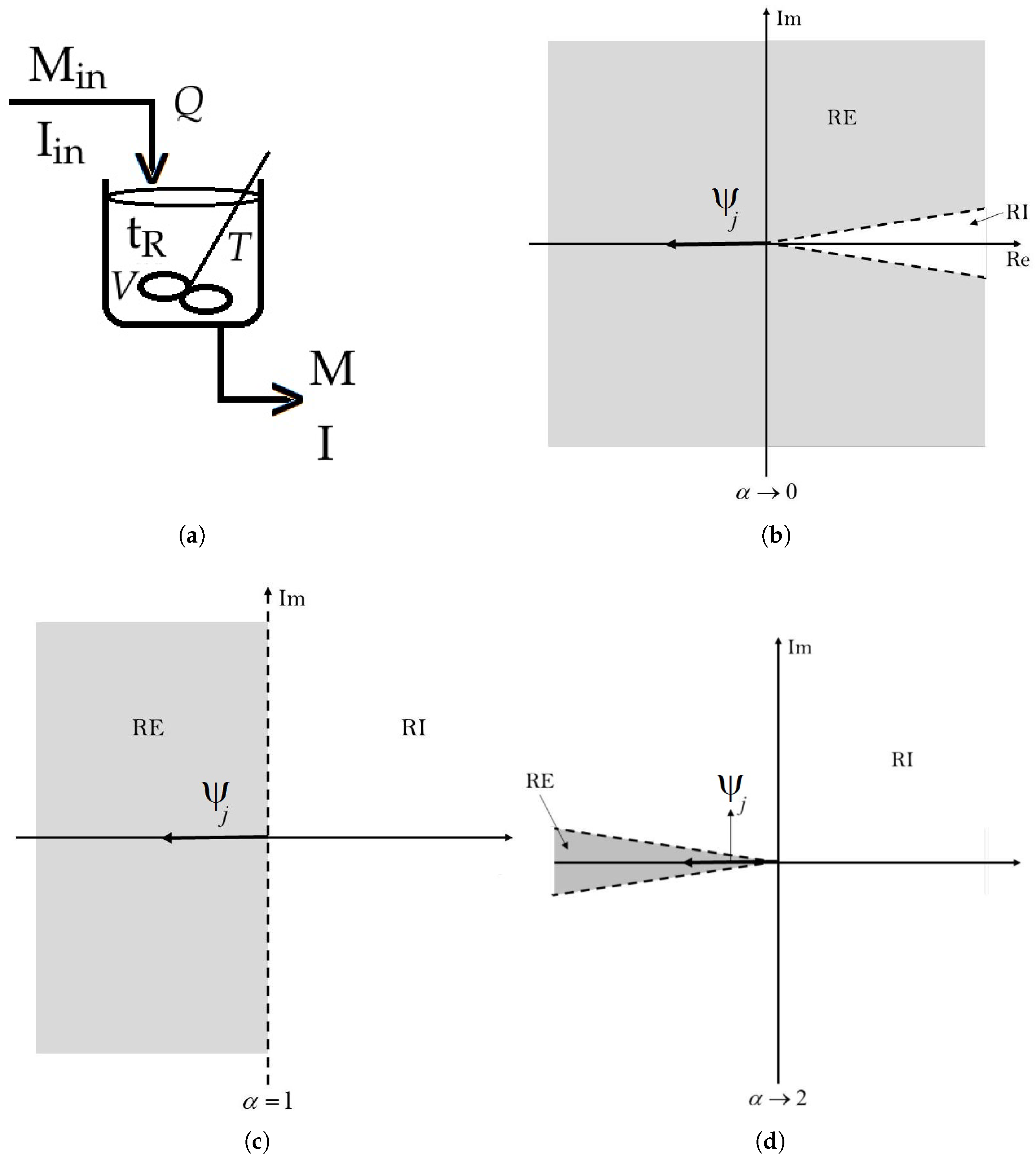
The Jacobian matrix of the linearised dynamical system is given by J Equation (41), and it is written in terms of some dimensionless parameters defined in the Appendix A.

$$J=\left(\begin{array}{cccc}-{\mathrm{a}}_1& 0& 0& 0\\ 0& -{\mathrm{a}}_6& -{\mathrm{a}}_7& 0\\ {\mathrm{a}}_3& 0& -{\mathrm{a}}_9& 0\\ 0& 0& {\mathrm{a}}_{11}& -1\end{array}\right)$$

(41)

The characteristic equation of the Jacobian matrix is as follows: ${\Psi }^4$ + 12,637 ${\Psi }^3$ + 40,930 ${\Psi }^2$ + 44,097 $\Psi$ + 15,803 = 0. The eigenvalues corresponding to the system are ${\Psi }_1=-1.0657,{\Psi }_2=-1.1737,{\Psi }_3=-12,634,$${\Psi }_4=-1$. As these eigenvalues are all real negative numbers, it can be concluded that the dimensionless integer-order dynamic model is asymptotically stable at its physically feasible equilibrium point. However, it should be noted that the magnitudes of the calculated eigenvalues vary significantly; ${\Psi }_1,{\Psi }_3$, and ${\Psi }_4$ are on the order of ${10}^{\circ }$, while ${\Psi }_2$ is on the order of ${10}^3$. In the context of chemical engineering, this indicates a high level of system stiffness; mathematically, this scenario is designated as an ill-conditioned system. This implies that small perturbations or variations in the input of the mathematical dynamic model (in this case, dimensionless time) lead to significant and large changes in the outputs of the mathematical model [49,50]. In our dynamic system, these outputs correspond to the dependent variables, specifically the five state variables: initiator and monomer conversions, free radical and polymer concentrations (all dimensionless), and the average molecular weight of weight ($M_w$) [1,51]. To ensure the asymptotic stability of the linearised dynamic system with fractional orders, it is essential to calculate the argument of the eigenvalues to satisfy the condition given by the Equation (8) as stated in Theorem 1. Given that all eigenvalues are negative real values, it follows that

$$arg\left({\Psi }_{\mathrm{j}}\right)=\pi \mathrm{j}=1,2,3,4.$$

Therefore, we identified three scenarios:

• When $\alpha$ lies within the open interval $(0,1)$, the mathematical analysis depicted in Figure 1b shows that as $\alpha$ approaches zero, the limit of $\alpha {\displaystyle \frac{\pi }{2}}$ as $\alpha$ tends to 0 is 0. Consequently, the stable region expands until it almost covers the entire complex plane, while the unstable region shrinks. As $\alpha$ approaches one, the limit of $\alpha {\displaystyle \frac{\pi }{2}}$ as $\alpha$ approaches 1 is ${\displaystyle \frac{\pi }{2}}$. In this case, the stable and unstable regions almost become equal in size, resembling the stability regions of a first-order system. Therefore, for this specific scenario, $\alpha {\displaystyle \frac{\pi }{2}}$ falls within the open interval $\left(0,{\displaystyle \frac{\pi }{2}}\right)$, where for any value of $\theta$ in $\alpha {\displaystyle \frac{\pi }{2}}$, $arg\left({\Psi }_j\right)=\pi$ is greater than $\theta$. $arg\left({\Psi }_{\mathrm{j}}\right)=\pi >\theta ,\forall \theta \in \left(0,{\displaystyle \frac{\pi }{2}}\right)$. Hence, we can conclude that Equation (8) is met in this case.
• When $\alpha$ equals 1, the fractional order system is transformed into an integer order system. In this case, $\alpha {\displaystyle \frac{\pi }{2}}={\displaystyle \frac{\pi }{2}}$, and the condition C is satisfied, which implies that $arg\left({\Psi }_{\mathrm{j}}\right)=\pi >{\displaystyle \frac{\pi }{2}}$. This situation is depicted in Figure 1c.
• For $\alpha$ ranging between 1 and 2, the subsequent mathematical examination holds, as shown in Figure 1d: as $\alpha$ approaches 1, ${lim}_{\alpha \to 0}\alpha {\displaystyle \frac{\pi }{2}}={\displaystyle \frac{\pi }{2}}$, and the stability regions have been previously elucidated in case 1; as $\alpha$ approaches 2, ${lim}_{\alpha \to 0}\alpha {\displaystyle \frac{\pi }{2}}=\pi$, leading to an expansion of the unstable region almost throughout the complex plane, while the stable region tends to shrink. Therefore, in this third scenario, $\alpha {\displaystyle \frac{\pi }{2}}$ is within the range $\left({\displaystyle \frac{\pi }{2}},\pi \right)$, where for every $\theta$ value of $\alpha {\displaystyle \frac{\pi }{2}}$, $arg\left({\Psi }_{\mathrm{j}}\right)=\pi$ exceeds it, indicating that

  $$arg\left({\Psi }_{\mathrm{j}}\right)=\pi >\theta \mathrm{for}\mathrm{all}\theta \in \left({\displaystyle \frac{\pi }{2}},\pi \right).$$

  (42)
  Therefore, we can infer that in this particular scenario, Equation (8) is also met. Given that the condition given by Equation (8) is satisfied in all three cases examined above, we can deduce that the fractional order dynamical system of the CSTR polymerisation reactor for poly(methyl methacrylate) is asymptotically stable in its physically feasible steady state. This observation does not imply that fractional calculus is neither essential nor intriguing to mathematically model the reactor under investigation in this study. These mathematical techniques enable the expansion or contraction of unstable regions based on operational requirements while also helping to define the boundaries of desirable and safe operation.

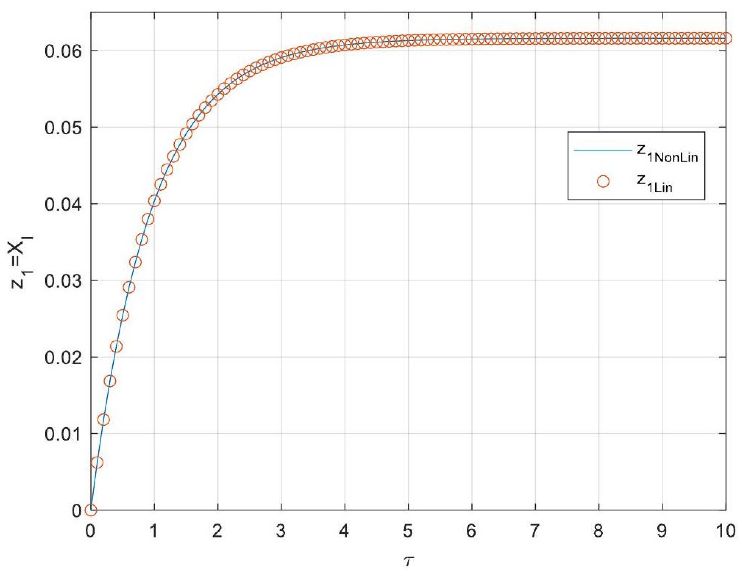
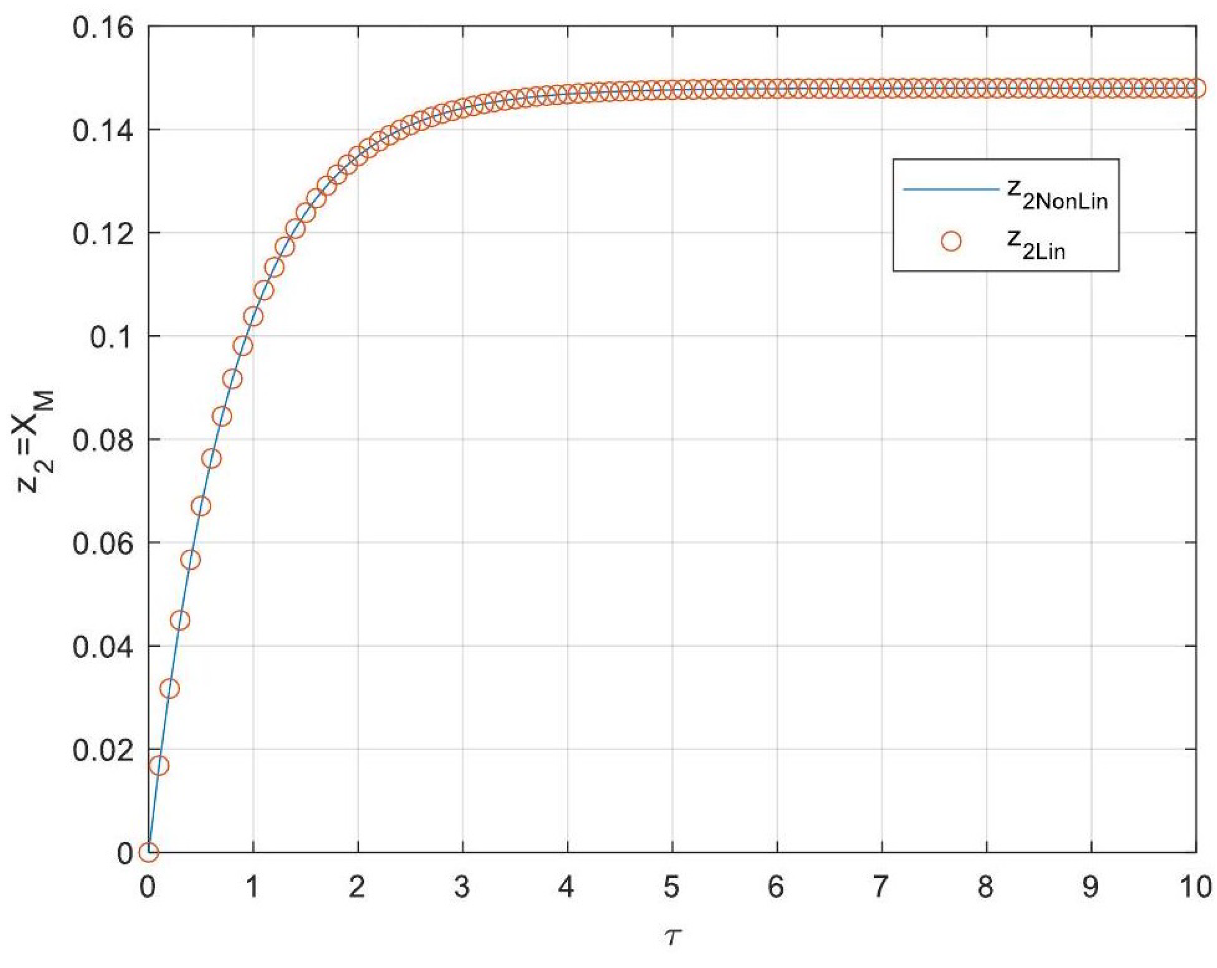
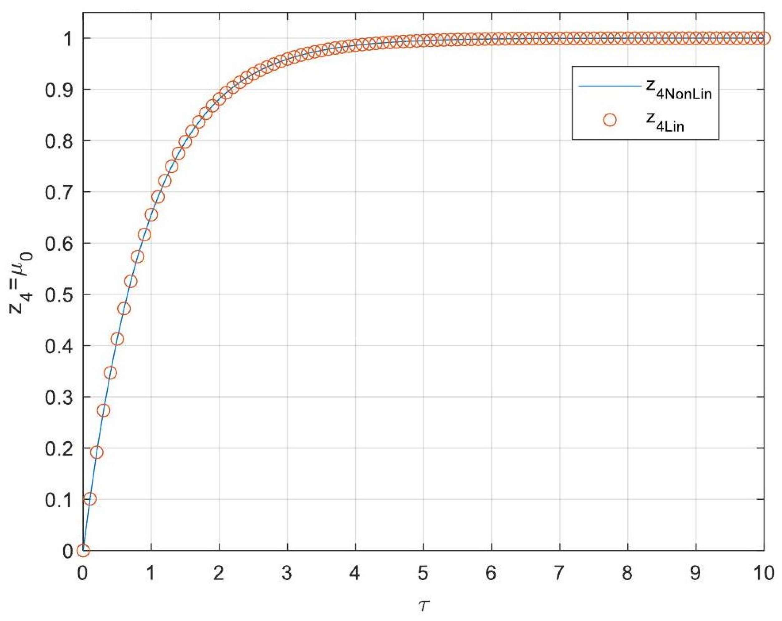
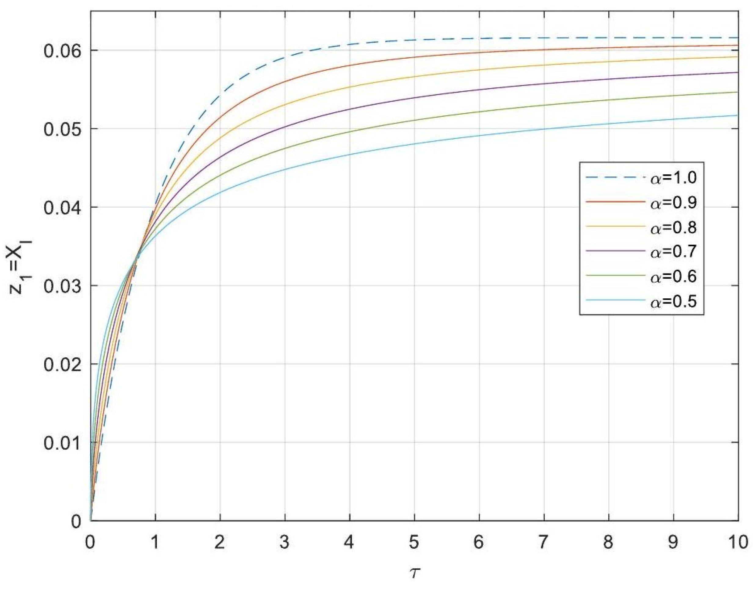
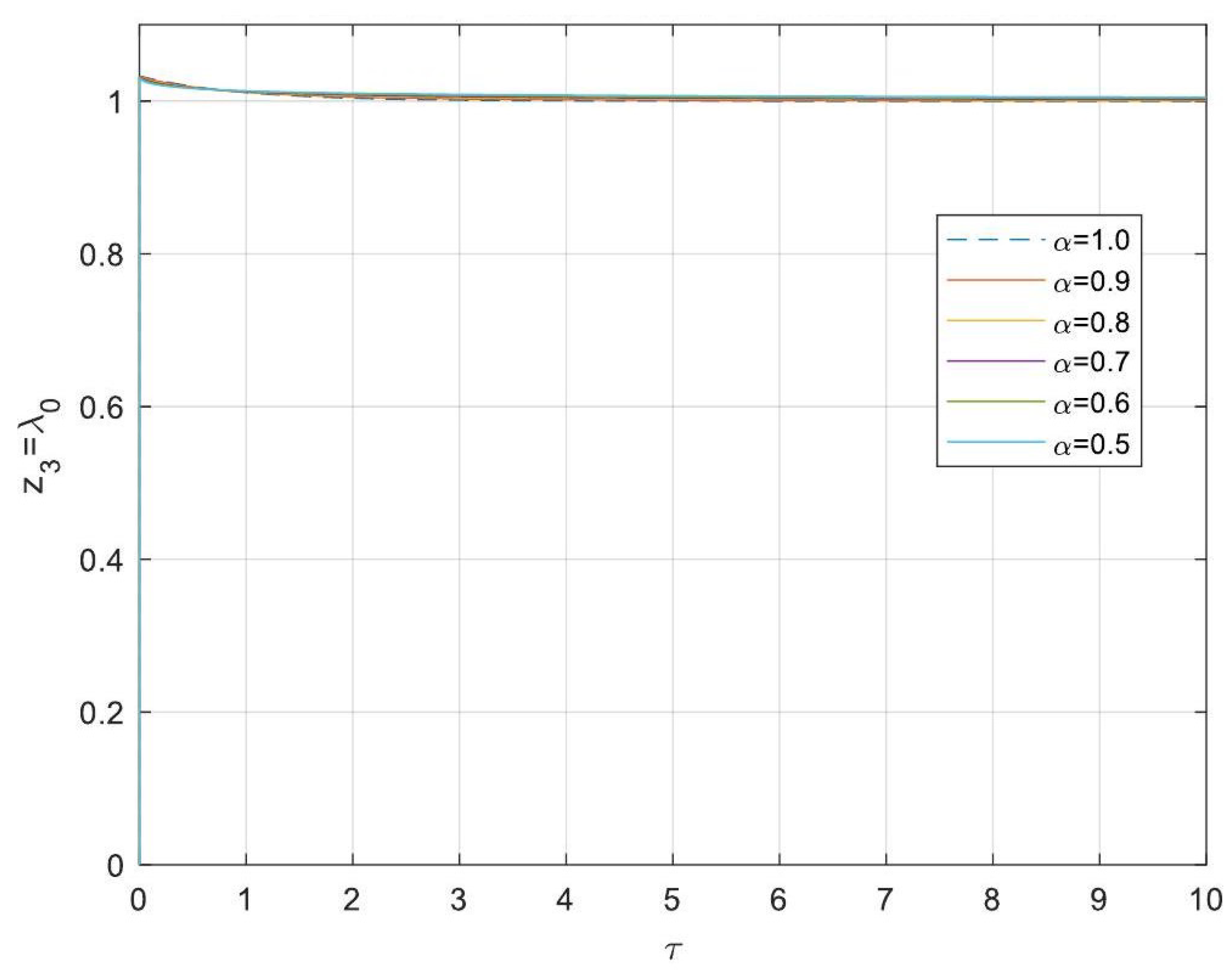
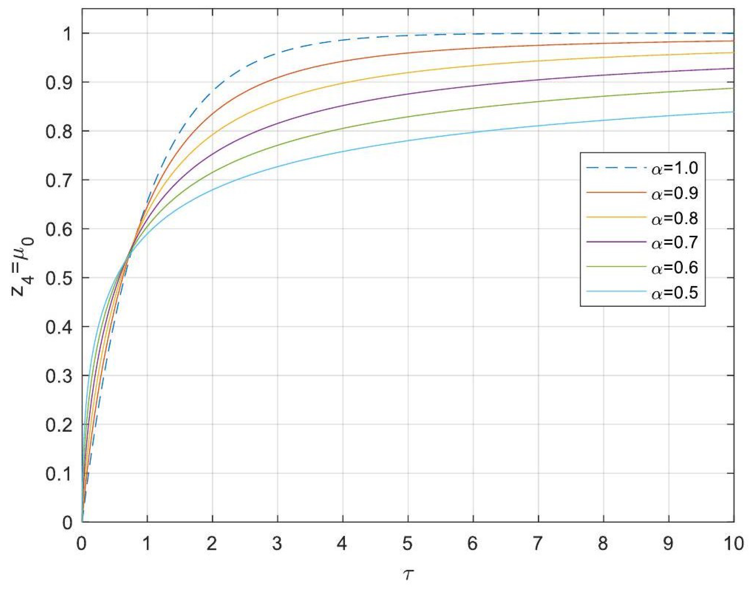
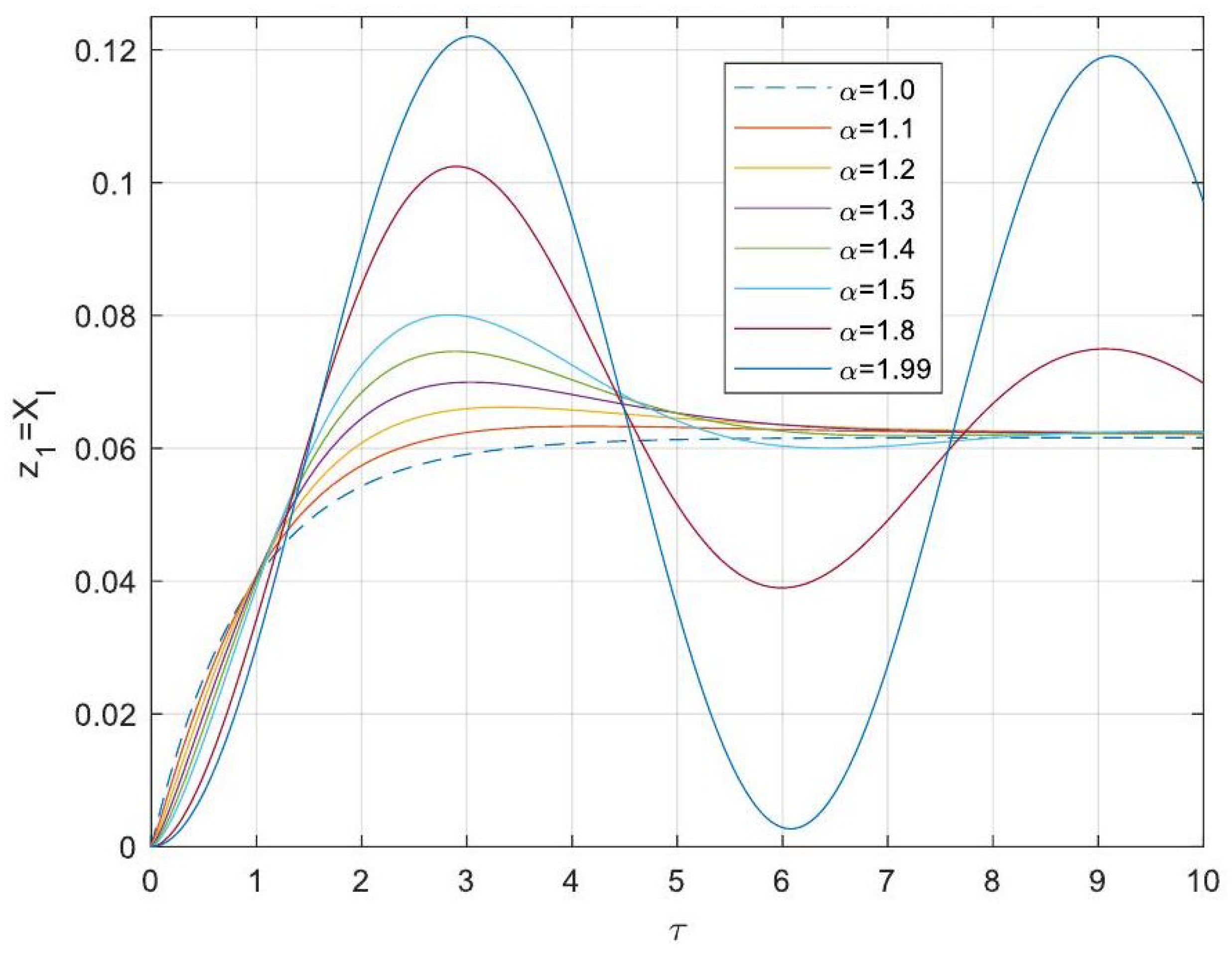
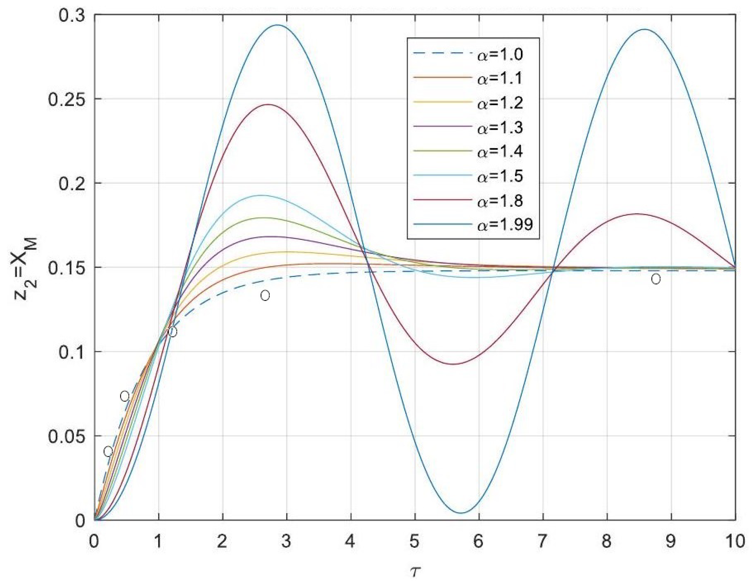
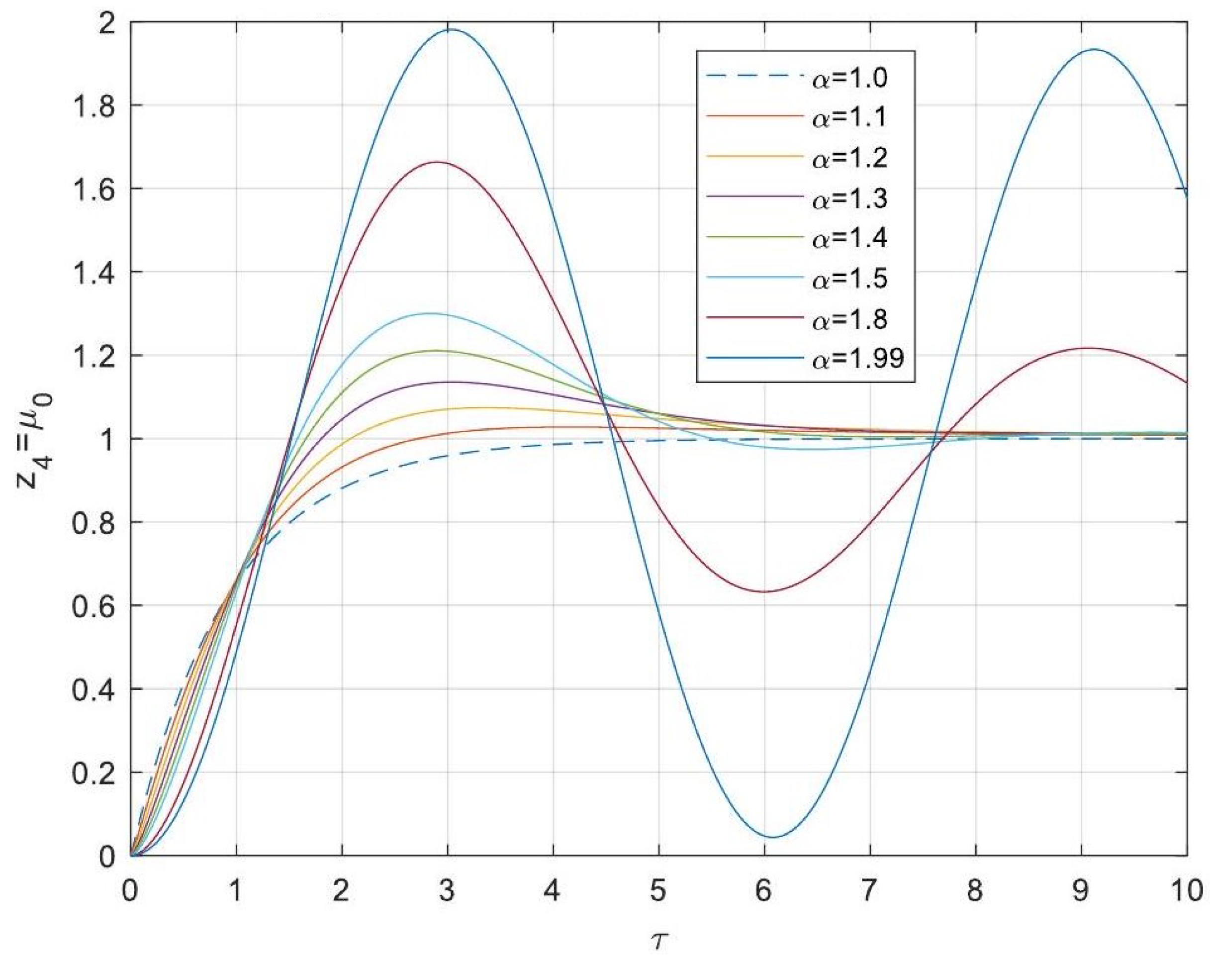
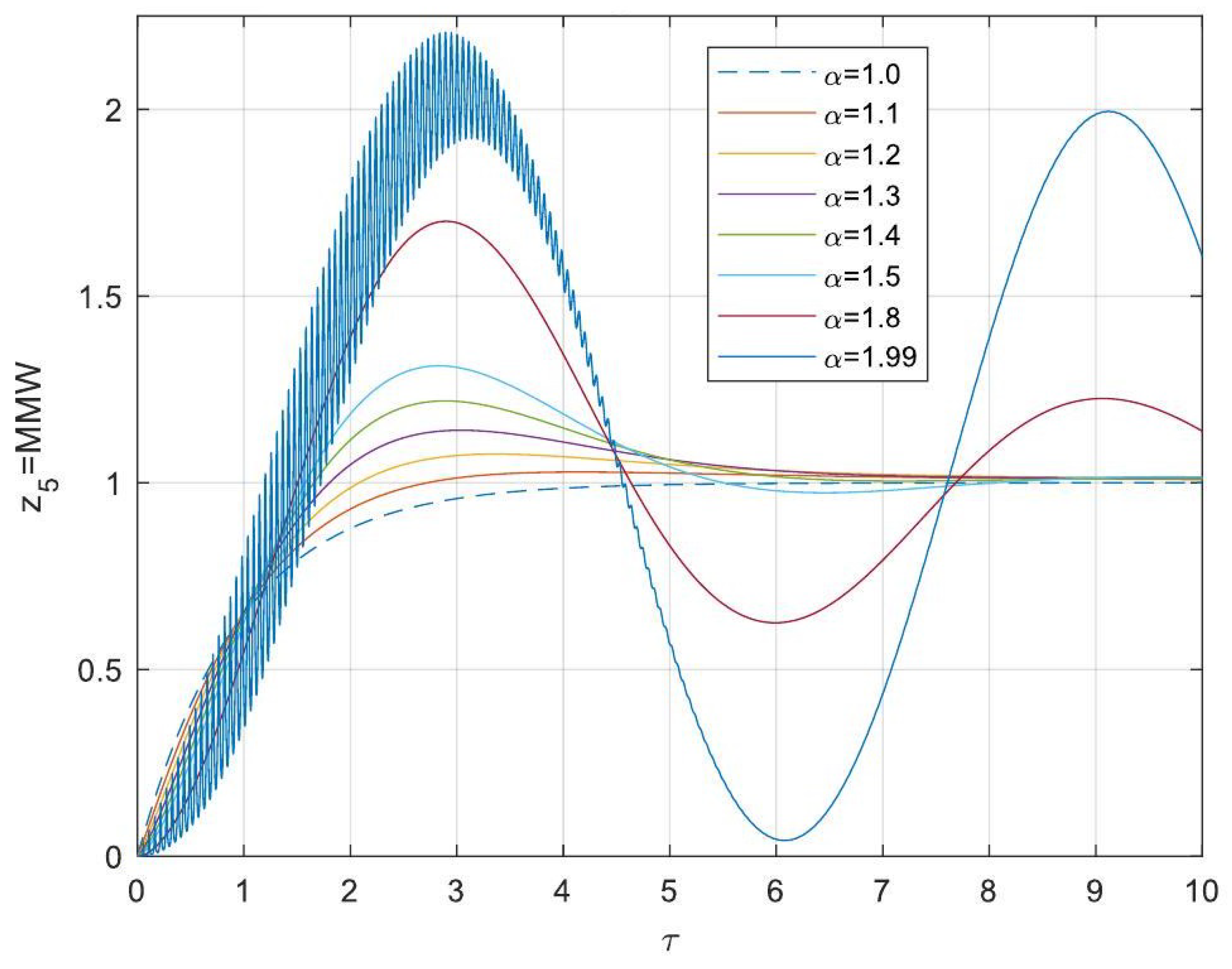
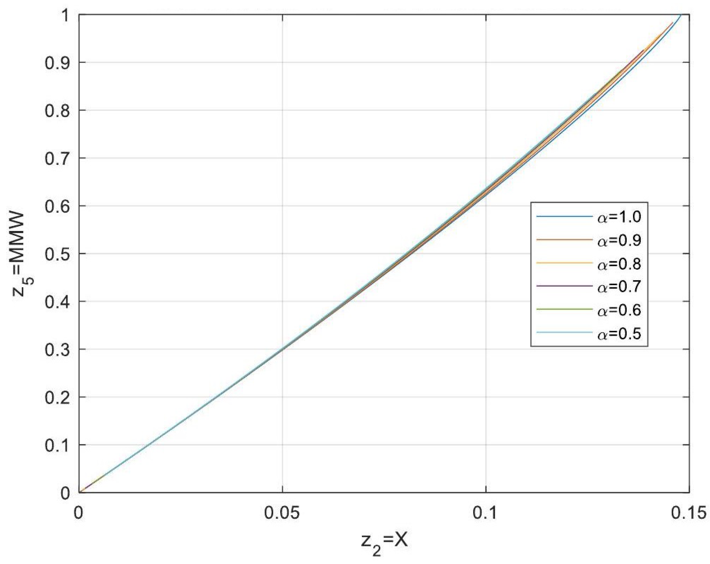
5.3. Analytical Solutions of the Linearised Model

The linearised integer order dynamic system arises when setting $\alpha =1$ in the linear fractional differential equation system Equations (22)–(31). Analytical solutions were derived using the Laplace transform [36,52] in conjunction with the Taylor first-order series [53]. These solutions are presented in the following way.

$$\begin{array}{ccc}\hfill \overline{I}\left(\tau \right)& =& \overline{z_1}\left(\tau \right)={\displaystyle \frac{1}{a_1}}+\left(1-{\displaystyle \frac{1}{a_1}}\right)e^{-a_1\tau }\hfill \end{array}$$

(43)

$$\begin{array}{cc}\hfill \overline{M}\left(\tau \right)=& {\overline{z}}_2\left(\tau \right)=a_{21}+a_{22}{e}^{-a_1\tau }+\hfill \\ & \left[1-\left(a_{21}+a_{22}+a_{23}\right)\right]e^{-a_6\tau }+a_{23}{e}^{-a_9\tau }\hfill \end{array}$$

(44)

$$\begin{array}{ccc}\hfill {\overline{\lambda }}_0\left(\tau \right)& =& {\overline{z}}_3\left(\tau \right)=a_{15}+a_{16}{e}^{-a_1\tau }+a_{17}{e}^{-a_9\tau }\hfill \end{array}$$

(45)

$$\begin{array}{ccc}\hfill {\overline{\mu }}_0\left(\tau \right)& =& {\overline{z}}_4\left(\tau \right)=a_{24}+a_{27}{e}^{-a_1\tau }+a_{28}{e}^{-a_9\tau }-\left(a_{24}+a_{27}+a_{28}\right)e^{-\tau }\hfill \end{array}$$

(46)

The linearised fractional model was also resolved using the Laplace transform, and the analytical solutions of the fractional differential equation system are given below.

$$\begin{array}{ccc}\hfill \overline{I}\left(\tau \right)& =& {\overline{z}}_1\left(\tau \right)={\displaystyle \frac{1}{a_1}}+\left(1-{\displaystyle \frac{1}{a_1}}\right)E_{\alpha }\left(-a_1{\tau }^{\alpha }\right)\hfill \end{array}$$

(47)

$$\begin{array}{cc}\hfill \overline{M}\left(\tau \right)=& {\overline{z}}_2\left(\tau \right)=a_{21}+a_{22}{E}_{\alpha }\left(-a_1{\tau }^{\alpha }\right)+\hfill \\ & \left[1-\left(a_{21}+a_{22}+a_{23}\right)\right]E_{\alpha }\left(-a_6{\tau }^{\alpha }\right)+a_{23}{E}_{\alpha }\left(-a_9{\tau }^{\alpha }\right)\hfill \end{array}$$

(48)

$$\begin{array}{ccc}\hfill {\overline{\lambda }}_0\left(\tau \right)& =& {\overline{z}}_3\left(\tau \right)=a_{15}+a_{16}{E}_{\alpha }\left(-a_1{\tau }^{\alpha }\right)+a_{17}{E}_{\alpha }\left(-a_9{\tau }^{\alpha }\right)\hfill \end{array}$$

(49)

$$\begin{array}{cc}\hfill {\overline{\mu }}_0\left(\tau \right)=& {\overline{z}}_4\left(\tau \right)=a_{24}+a_{27}{E}_{\alpha }\left(-a_1{\tau }^{\alpha }\right)+a_{28}{E}_{\alpha }\left(-a_9{\tau }^{\alpha }\right)-\hfill \\ & \left(a_{24}+a_{27}+a_{28}\right)E_{\alpha }\left(-{\tau }^{\alpha }\right)\hfill \end{array}$$

(50)

The analytical solution was obtained by the Mittag-Leffler function, and it is shown as follows.

$$\begin{array}{ccc}\hfill E_{\alpha }\left(-a_1{\tau }^{\alpha }\right)& =& \sum _{m=0}^{\infty }{\displaystyle \frac{{\left(-a_1{\tau }^{\alpha }\right)}^m}{\mathrm{\Gamma }(m\alpha +1)}}\hfill \end{array}$$

(51)

$$\begin{array}{ccc}\hfill E_{\alpha }\left(-a_6{\tau }^{\alpha }\right)& =& \sum _{m=0}^{\infty }{\displaystyle \frac{{\left(-a_6{\tau }^{\alpha }\right)}^m}{\mathrm{\Gamma }(m\alpha +1)}}\hfill \end{array}$$

(52)

$$\begin{array}{ccc}\hfill E_{\alpha }\left(-a_9{\tau }^{\alpha }\right)& =& \sum _{m=0}^{\infty }{\displaystyle \frac{{\left(-a_9{\tau }^{\alpha }\right)}^m}{\mathrm{\Gamma }(m\alpha +1)}}\hfill \end{array}$$

(53)

$$\begin{array}{ccc}\hfill E_{\alpha }\left(-{\tau }^{\alpha }\right)& =& \sum _{m=0}^{\infty }{\displaystyle \frac{{\left(-{\tau }^{\alpha }\right)}^m}{\mathrm{\Gamma }(m\alpha +1)}}\hfill \end{array}$$

(54)

The dimensionless parameters ${\mathrm{a}}_{13}$ to ${\mathrm{a}}_{29}$ are introduced in the Appendix A and lack physical significance. In the set Equations (47)–(49) and (51)–(53), conditions $Re\left(\alpha \right)>0$ and $0<\alpha <2$ are imposed. The former requirement is related to the Mittag-Leffler function definition, while the latter is related to the integer order of the linearised dimensionless system. When $\alpha =1$, the explicit analytical solutions in Equations (47)–(49) and (51)–(53) simplify to match the solutions of the linearised integer order system described in Equations (43)–(45). Therefore, solutions S and $\mathrm{P}$ represent a potential extension of the solutions for Equations (47)–(49) and where the exponential functions are replaced by the Mittag-Leffler functions of one parameter in Equations (43)–(45).

Figure 2, Figure 3, Figure 4 and Figure 5 represent the comparison between the dynamic responses of the original nonlinear dimensionless system and its linearised counterpart to evaluate the precision of the linear approximation. In Figure 2, a comparison is presented between a linear dynamic response obtained analytically using Equation (43) and a numerical dynamic response computed using ode15s, given the linearity of Equation (43). Based on these figures, the dynamic responses of the nonlinear dimensionless integer order mathematical model closely resemble those of the corresponding linear dimensionless integer order model when visually considering all four state variables. Nevertheless, for a more detailed analysis, it is essential to quantify the deviations of the integer-order linearised model from the nonlinear integer-order model using the arithmetic mean of the deviations of nonlinearity, which is defined as follows:

$${\overline{\mathrm{D}}}_{\mathrm{j}}=\sum _{\mathrm{m}=1}^{{\mathrm{N}}_{\mathrm{d}}}{\displaystyle \frac{{\mathrm{z}}_{\mathrm{jNonlin}}-{\mathrm{z}}_{\mathrm{jLin}}}{{\mathrm{N}}_{\mathrm{d}}}},j=1,2,3,4$$

(55)

where ${\mathrm{N}}_{\mathrm{d}}$ represents the number of data points used for the plot. In

Table 5. Discrepancies between the linearised integer-order dimensionless model and the nonlinear model.

Symbol for Mean Deviation Value	Description	Deviation Value
${\overline{\mathrm{D}}}_1$	Initiator conversion	$5.1489\times {10}^{-8}$
${\overline{D}}_2$	Monomer conversion	$2.7390\times {10}^{-5}$
${\overline{D}}_3$	Dimensionless free
	concentration of radicals	$2.3367\times {10}^{-5}$
${\overline{D}}_4$	Dimensionless
	polymer concentration	$8.3951\times {10}^{-7}$

, the numerical values of these deviations mentioned in the preceding paragraph are displayed for each state variable.

As shown in Table 5, the nonlinear deviations are sufficiently low, on the order of ${10}^{-5}$ for both monomer conversion and dimensionless free radical concentration, ${10}^{-7}$ for dimensionless polymer concentration, and ${10}^{-8}$ for initiator conversion. This suggests two key observations regarding our dimensionless original integer order system with nonlinearity: first, both graphically and numerically, the linearisation around its physically feasible steady state is successful; second, as indicated by the stability analysis results and Figure 2, Figure 3, Figure 4 and Figure 5, the system is asymptotically stable at its physically attainable steady state.

Based on the data presented in Figure 6, Figure 7, Figure 8, Figure 9 and Figure 10, it can be observed that for derivative orders $\alpha$ within the range of $(0,1)$, lower values of the derivative order lead to higher initiator and monomer conversions, as well as increased concentrations for free radicals ${\lambda }_0$ and polymers ${\lambda }_0$. This trend holds until a certain point in time when the behaviour switches. For $\alpha$ values between 0.5 and 1, this reversal typically occurs at a dimensionless time of approximately between 0.6 and 0.8. However, from Figure 11, Figure 12, Figure 13, Figure 14, Figure 15, Figure 16 and Figure 17, for $\alpha$ values between 1 and 2, this reversal occurs at a dimensionless time approximately between 1 and 1.4. When $\alpha$ is less than 1, the dynamic responses tend towards asymptotic stability. In contrast, for $\alpha$ values between 1 and 2, the responses exhibit oscillatory behaviour. It is important to note that the presence of oscillations does not indicate instability in the fractional-order dynamic model. As depicted in Figure 11, Figure 12, Figure 13, Figure 14 and Figure 15 for values of $\alpha$ between 1 and 1.8, the amplitude of oscillations decreases over time until they eventually vanish, as can be observed in Figure 13 for the concentration of dimensionless free radicals.

In Figure 10 and Figure 15, the average molecular weight of the weight shows a pattern similar to that outlined in the previous section except for $\alpha =1.99$. According to Figure 8, where $0.5\le \alpha <1$, the dimensionless concentration of free radicals shows the typical behaviour reported in the literature [1,51] at the beginning; this state variable increases freely reaching a maximum and after this moment it becomes asymptotically stable. The dynamic responses to the concentration of free radicals illustrated in Figure 13 demonstrate the impact of fractional-order derivatives on the behaviour of the CSTR system. For values of $1\le \alpha <2$, the system exhibits oscillatory responses, with amplitudes gradually decreasing over time. This behaviour stems from the inherent memory effects of fractional derivatives, which allow the system to incorporate past states into its evolution. Unlike integer-order models that predict purely exponential decay, fractional-order models capture intermediate behaviours more effectively, leading to improved accuracy in representing the polymerisation process. These results reinforce the applicability of fractional calculus in chemical reaction engineering, particularly for the stability and performance of the process.

According to Figure 16, for any derivative order $0.5\le \alpha <1$, the molecular weight average of weight does not have any effect on monomer conversion. The opposite behaviour is presented on unstable attractors depicted in Figure 17; the greater $\alpha$, the greater these effects, since the greater $\alpha$, the greater the oscillations, even if they disappear at the end. It is important to note that the observed oscillations in Figure 13, Figure 14, Figure 15, Figure 16, Figure 17, Figure 18 and Figure 19 are not a consequence of the numerical method but rather an inherent characteristic of the behaviour of the system for certain fractional-order values $1<\alpha <2$. The stability analysis remains valid as it is based on the local properties of the system near the steady state, where the nonlinear system is continuously differentiable. The numerical and analytical solutions are consistent, confirming that the stability properties are independent of the solution approach.

The results obtained in the previous paragraphs allow us to confirm and reinforce that for all $0<\alpha <2$ values studied, our linearised fractional-order nonlinear system is asymptotically stable in its physically stable state. Based on the analyses conducted in the preceding five paragraphs to enhance the effects and performance results for the anticipated monomer conversion, the dimensionless polymer concentration, and consequently, the molecular weight-average weight, it is recommended to work within regions corresponding to values of $1<\alpha <2$. However, it is crucial not to exceed excessively high values within this range, as the system can become unstable at such levels of $\alpha$. It is important to note that as $\alpha$ increases, the stability of the system decreases. To avoid operating in these unstable zones and determine the upper limits of safe operation for each state variable, Figure 18, Figure 19, Figure 20, Figure 21, Figure 22, Figure 23, Figure 24 and Figure 25 were plotted using the maximum values of the state variable from Figure 11, Figure 12, Figure 13 and Figure 14. These figures delineate the performance regions and operational boundaries from a chemical engineering point of view, collectively referred to as performance maps.

The highest values of the permitted derivative order for the safe and optimal operation of the reactor in chemical engineering are as follows: Based on Figure 23, Figure 24 and Figure 25, the value of $\alpha$ is 1.3. This value corresponds to the points where the initiator, monomer, and polymer concentrations reach their respective minima.

It was previously mentioned that when considering derivative orders within the open interval $(1,2)$, the five state variables exhibit oscillations. However, despite this behaviour, it has been proven through theorems and dynamic responses that the system remains asymptotically stable. Therefore, the interval $(1,1.3]$ is identified as the operational range of derivative order in which the fractional order system demonstrates superior performance compared to the integer order model in terms of initiator conversion, monomer conversion, dimensionless concentration of free radicals, and average molecular weight. On the other hand, the interval $(1,1.2]$ is the derivative order range in which the fractional-order system outperforms the corresponding integer-order model only in terms of polymer concentration.

To address instabilities within the optimal operating range of $(1,1.3]$ for initiator conversion, monomer conversion, dimensionless concentration of free radicals and average molecular weight of the weight, and $(1,1.2]$ for dimensionless concentration of polymers, we can adjust the PID controllers. These controllers are advantageous as they do not account for constraints and are simpler to manage. However, operating beyond these specified intervals poses a risk of disrupting plant operations and potentially compromising the quality of the polymer product, even with PID controller tuning. Beyond these operational thresholds, the system tends to become less stable and more prone to instability. It is important to note that for the five state variables, higher derivative orders lead to increased system instability due to the greater occurrence of oscillations.

Based on the analysis conducted in the preceding two paragraphs supported from Figure 18, Figure 19, Figure 20, Figure 21, Figure 22, Figure 23, Figure 24 and Figure 25, it is recommended that the derivative orders for each variable state are adjusted as follows to achieve better conversions: 1.3 for monomer conversion and average molecular weight of weight; 1.2 for dimensionless polymer concentration; and 1.3 for initiator conversion and dimensionless concentration of free radicals. However, this objective cannot be met using a commensurate order system, as described in this study. To address this issue within a commensurate order system, it is necessary to model it with a derivative order of $\alpha =1.2$. A proposal to address this challenge is briefly outlined in the conclusion section as its detailed development is beyond the scope of this paper. Dynamic reactions were determined using analytical solutions denoted by Equations (43)–(51) and were visualised using MATLAB (R2018b)^TM programming language.

Fractional Flow Analysis.Figure 23, Figure 24 and Figure 25 present the fractional flow characteristics of the initiator, monomer, and polymer, respectively, as functions of the derivative order $\alpha$ in the range [1,2). In Figure 23, the results of the fractional flow of the initiator reveal that the fractional-order models facilitate smoother fractional flow dynamics for the initiator. As $\alpha$ increases, the oscillations in flow dynamics become more pronounced, highlighting the trade-off between performance enhancement and stability. In Figure 24, the fractional flow derivatives of the monomer expand the range of operating conditions under which the optimal monomer flow is achieved. However, similar to the initiator flow, increasing $\alpha$ introduces oscillations that require careful monitoring to maintain process efficiency. Finally, in Figure 25, the results of the fractional polymer flow are shown. Fractional derivatives lead to improved polymer flow dynamics, with higher flow rates observed for $\alpha$ values around 1.2–1.3. Beyond this range, oscillations become more prominent and the system’s response tends toward instability. The fractional flow analysis underscores the potential of fractional-order models to optimise flow characteristics while expanding the operational boundaries of the reactor. However, these benefits are contingent on maintaining derivative orders within a safe and stable range. Exceeding $\alpha >1.3$ for most variables leads to a decrease in stability and potential risks to reactor operation.

6. Conclusions

This study presents a comprehensive analysis of nonlinear fractional-order dynamic models applied to a continuous stirred tank reactor (CSTR) for poly(methyl methacrylate) (PMMA) polymerisation. Using fractional calculus, analytical solutions were derived using the Laplace transform combined with Taylor series expansion. Stability analyses demonstrated that the system exhibits asymptotic stability in its physically feasible steady state, with variations in fractional derivative orders significantly impacting both stability regions and process performance. Key findings include the following.

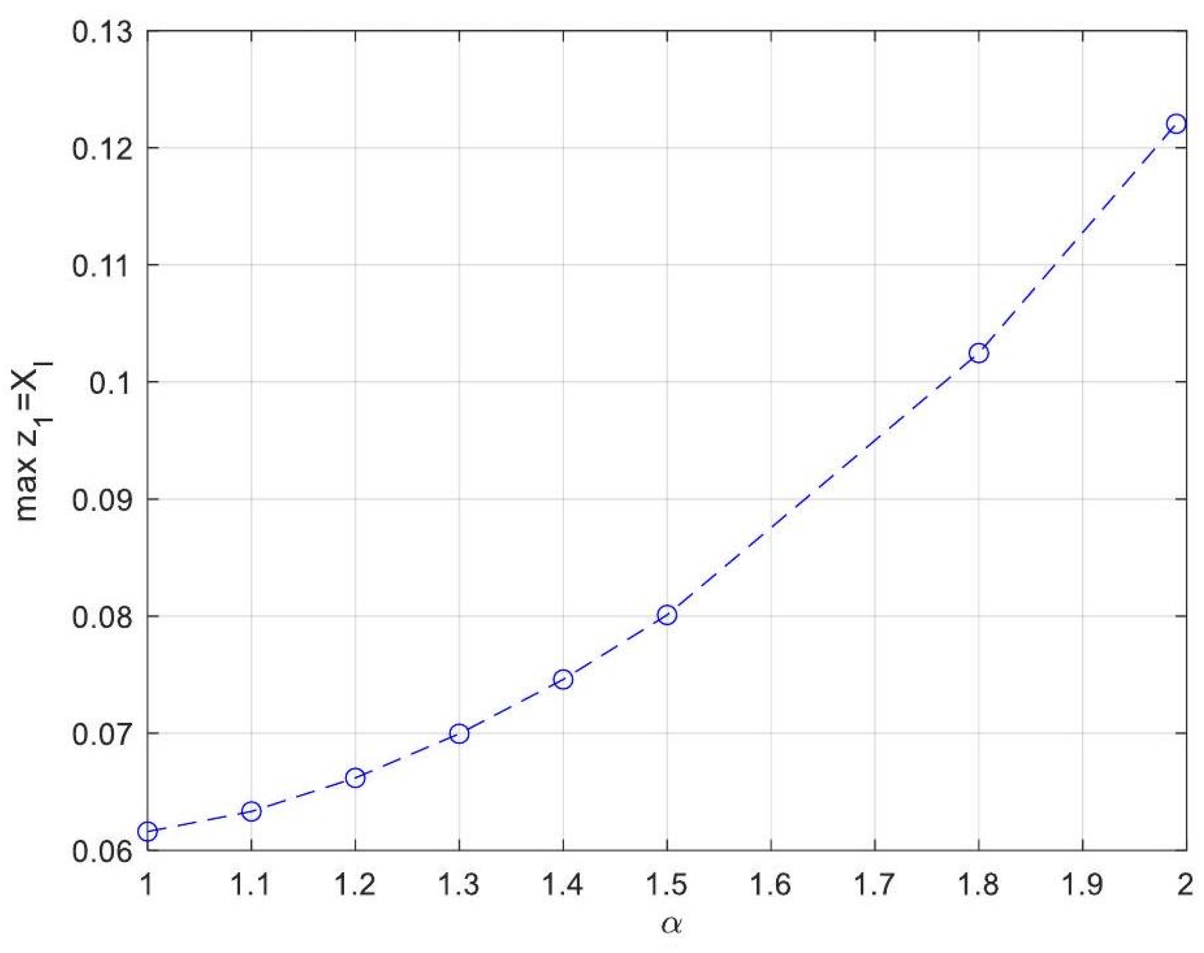
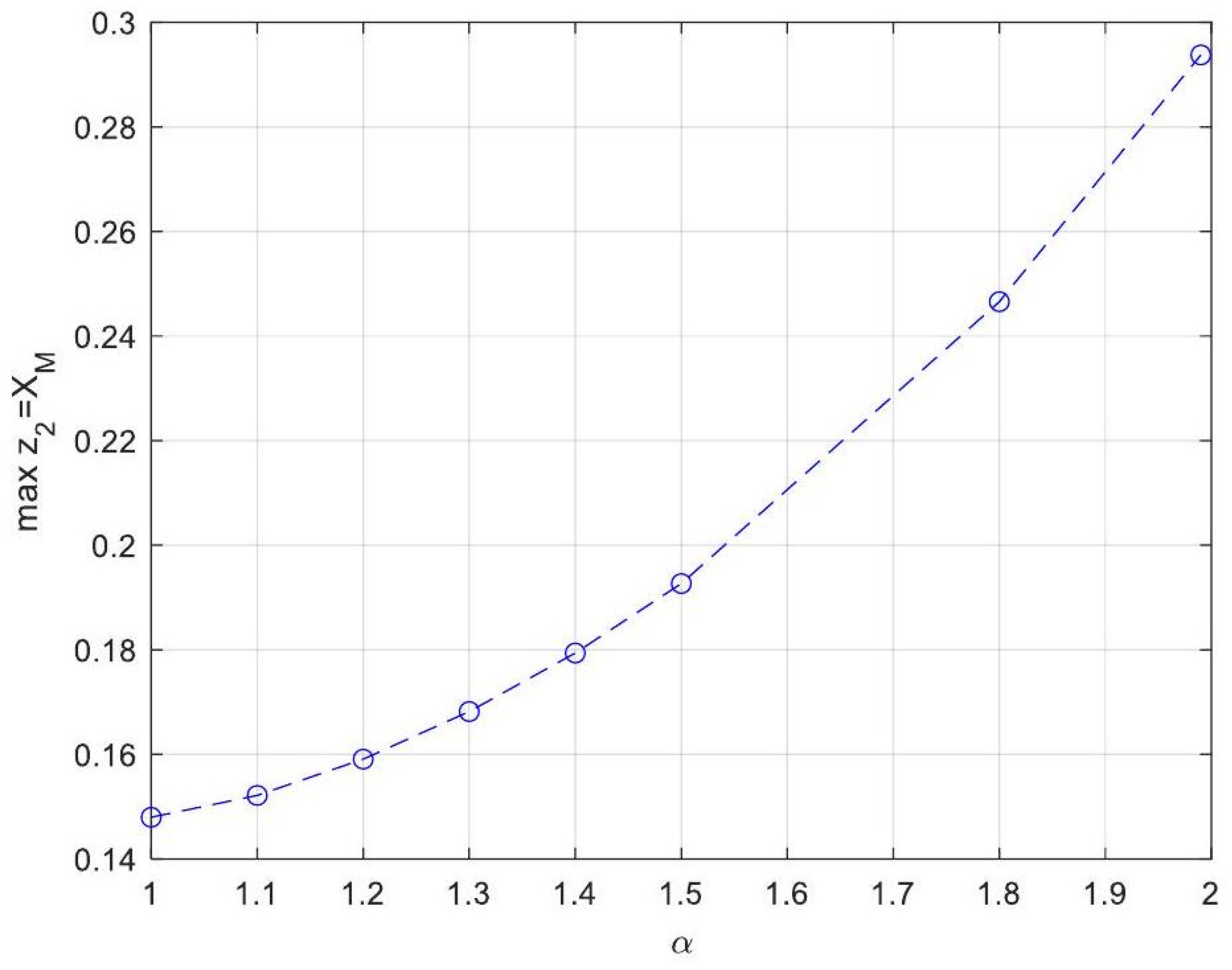
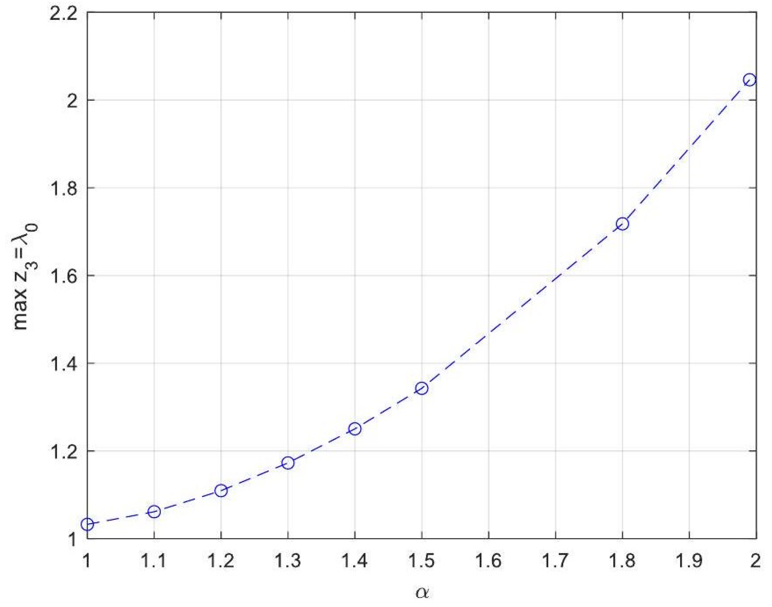
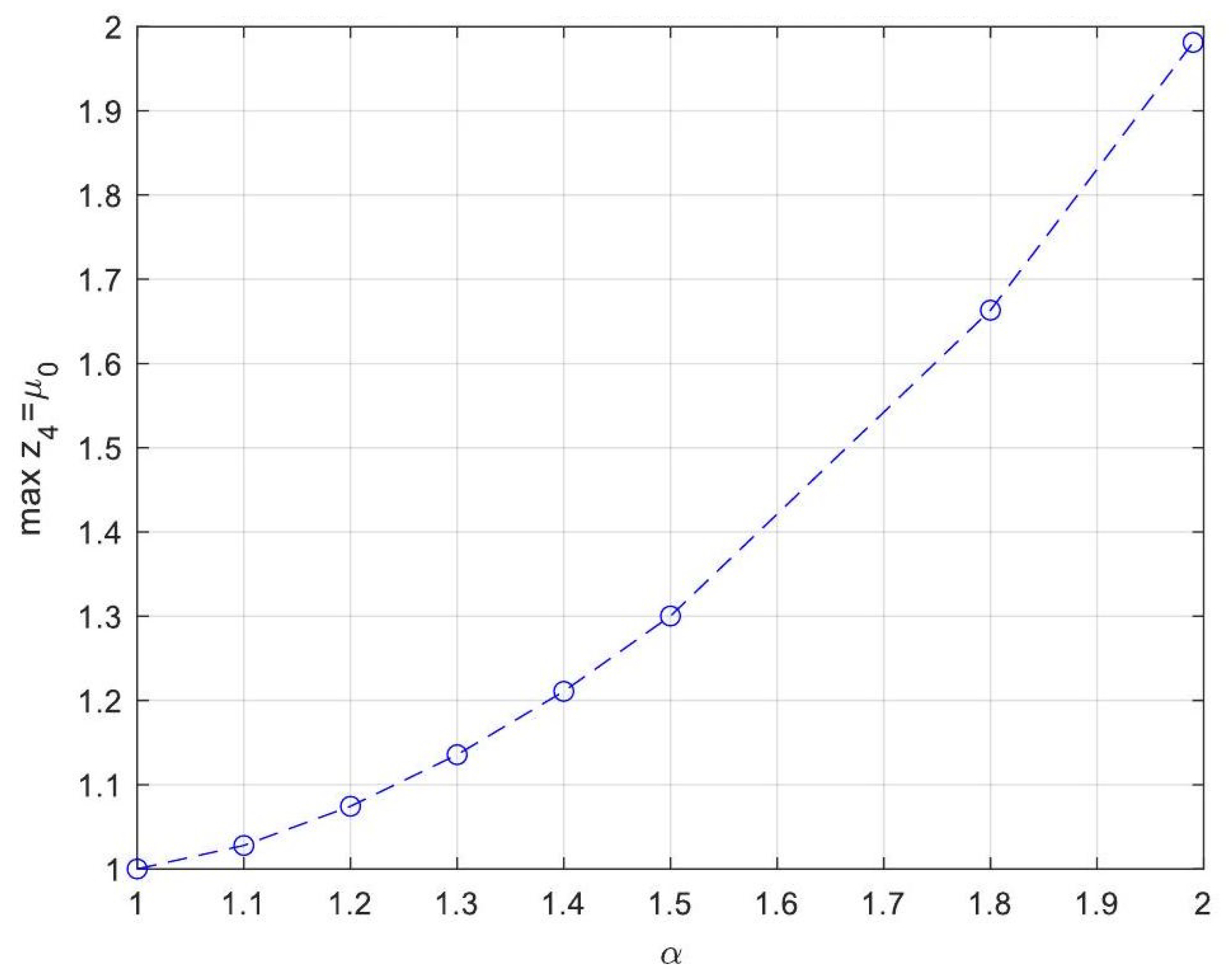
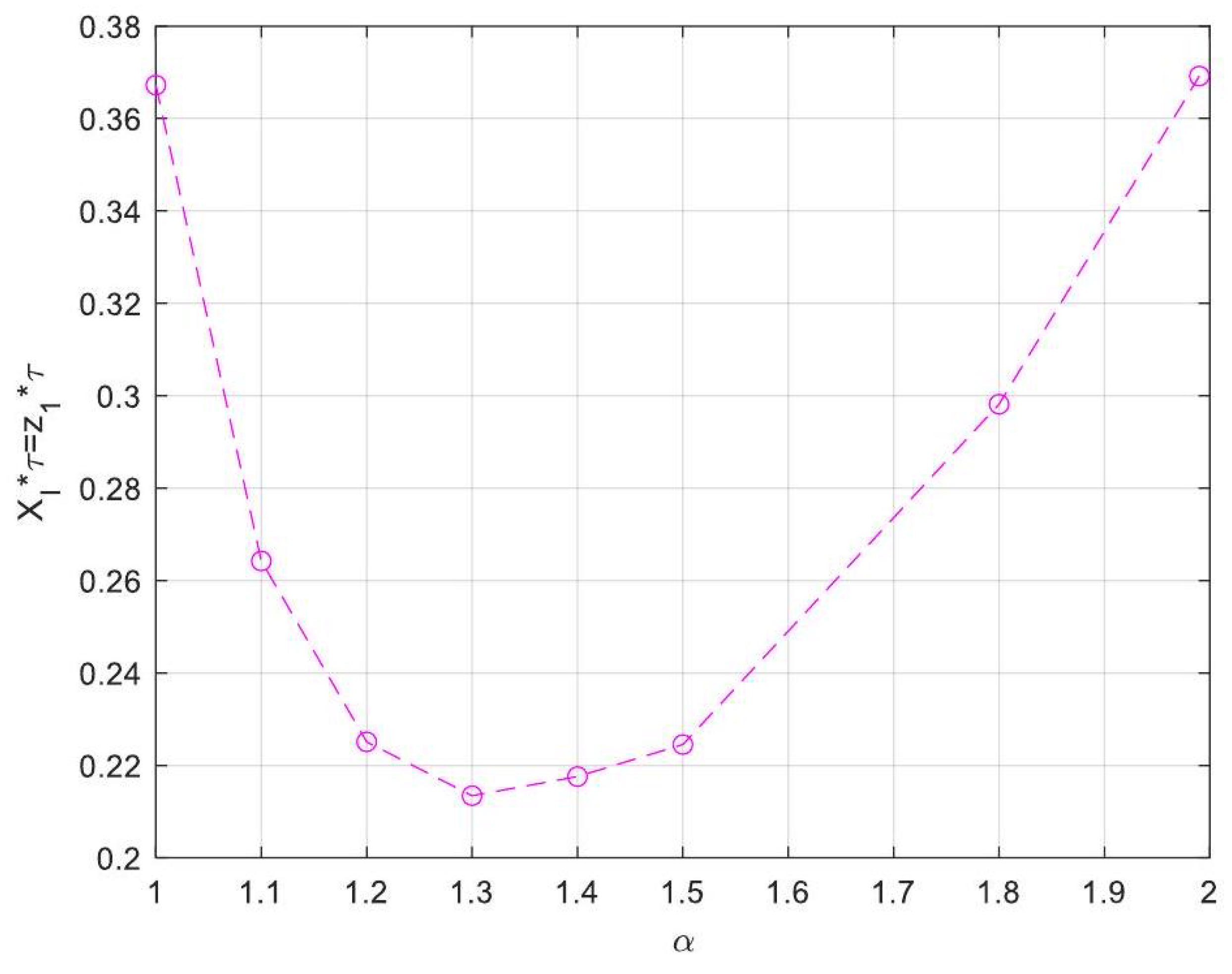
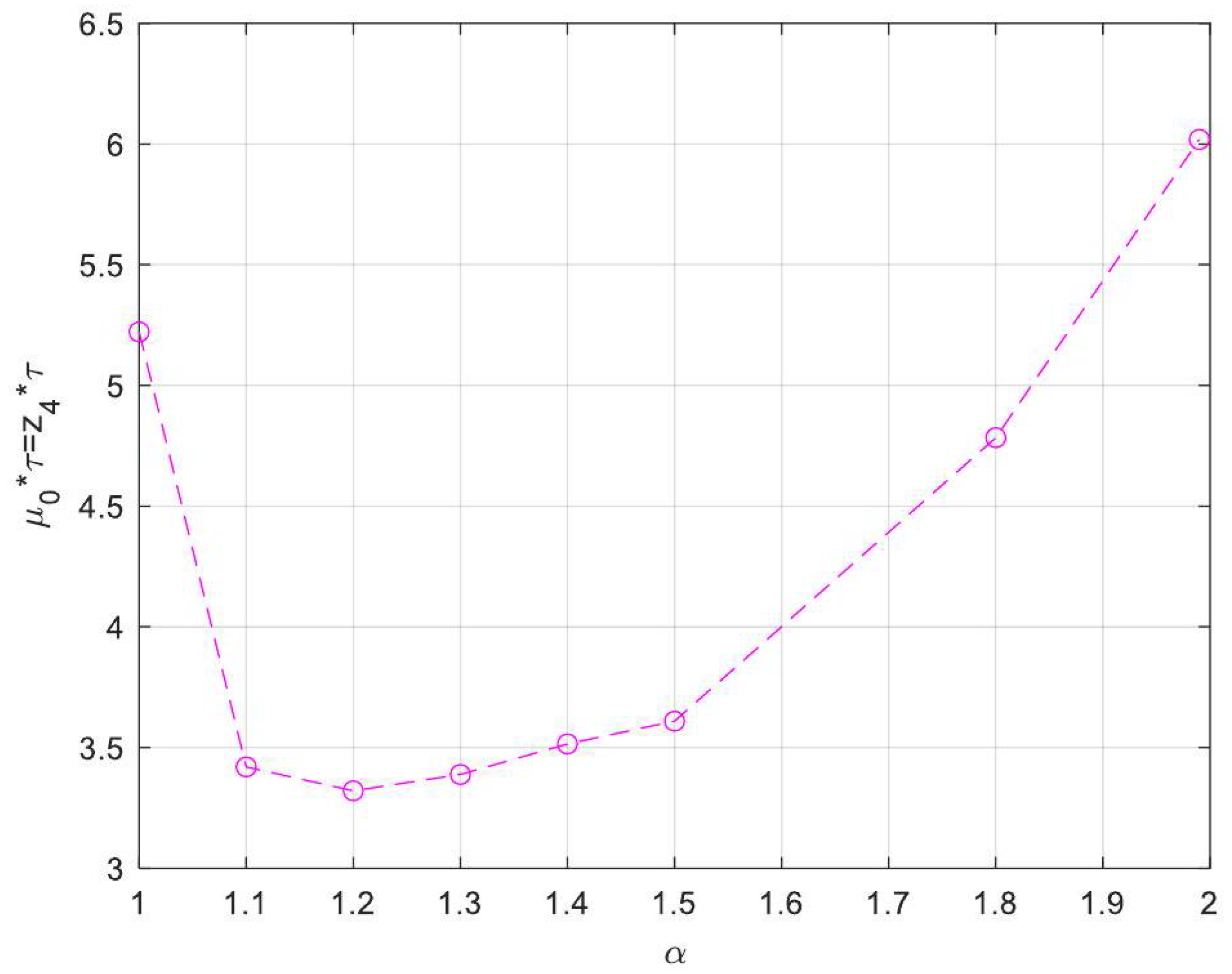
• Enhanced Process Performance with Fractional Operators: Fractional-order derivatives enable improved monomer conversion, polymer concentration, and weight average molecular weight, particularly for derivative orders in the range (1, 1.3]. This provides a notable advantage over integer-order systems, which are limited in stability region adaptability.
• Operational Windows for Optimal Performance: This study identified different operating windows for safe and effective reactor operation. Specifically: For initiator and monomer conversions, free radical concentration and weight-average molecular weight, the optimal derivative order lies in the range (1, 1.3]. And for polymer concentration, the optimal range narrows to (1, 1.2]. Beyond these ranges, increased derivative orders lead to instability and a potential degradation of product quality.
• Asymptotic Stability Across Derivative Ranges: Fractional-order systems exhibit a broader stability region for derivative orders in (0, 1), while narrowing as the derivative order approaches 2. This flexibility allows the system to be tuned for specific performance objectives without compromising stability.
• Comparison Between Fractional- and Integer-Order Models: Fractional-order models outperformed their integer-order counterparts in terms of stability, precision, and operational adaptability. The analytical solutions derived for fractional systems generalised those of the models of integer order, offering a deeper insight into reactor dynamics.

Despite these advancements, this study highlights the inherent limitation of commensurate systems, where a single derivative order applies uniformly to all state variables. A non-commensurate system, where each variable has a distinct derivative order, may provide further opportunities to optimise performance and enhance stability. However, this prospect requires further investigation beyond the scope of this work.

Future research directions could explore the integration of non-commensurate fractional order systems, advanced control strategies (e.g., fractional PID controllers), and the experimental validation of the proposed mathematical models. By addressing these challenges, fractional calculus can continue to play a transformative role in the optimisation of chemical engineering processes.

References

1. Chiu, W.; Carrat, G.; Soong, S. A Computer Method for the Gel Effect in Free Radical Polymerization. Macromolecules 1983, 16, 348–357. [Google Scholar] [CrossRef]
2. Maschio, G.; Moutier, C. Polymerization reactor: The influence of “gel effect” in batch and continuous solution polymerization of methyl methacrylate. J. Appl. Polym. Sci. 1989, 37, 825–840. [Google Scholar] [CrossRef]
3. Zavala, V.; Flores, A.; Vivaldo-Lima, E. Dynamic optimization of a semi-batch reactor for polyurethane production. Chem. Eng. Sci. 2005, 60, 3061–3079. [Google Scholar] [CrossRef]
4. Flores-Tlacuahuac, A.; Zavala-Tejeda, V.; Saldívar-Guerra, E. Complex Nonlinear Behavior in the Full-Scale High-Impact Polystyrene Process. Ind. Eng. Chem. Res. 2005, 44, 2802–2814. [Google Scholar] [CrossRef]
5. Zavala-Tejeda, V.; Flores, A.; Vivaldo-Lima, E. The bifurcation behavior of a polyurethane continuous stirred tank reactor. Chem. Eng. Sci. 2006, 61, 7368–7385. [Google Scholar] [CrossRef]
6. Heymans, N. Fractional Calculus Description of Non-Linear Viscoelastic Behaviour of Polymers. Nonlinear Dyn. 2004, 38, 221–231. [Google Scholar] [CrossRef]
7. Mainardi, F. Fractional Calculus: Theory and Applications. Mathematics 2018, 6, 145. [Google Scholar] [CrossRef]
8. Kilbas, A.; Srivastava, H.; Trujillo, J. Theory and Applications Of Fractinal Differential Equations; Elsevier: Amsterdam, The Netherlands, 2006; Volume 204. [Google Scholar] [CrossRef]
9. Shen, X. Applications of Fractional Calculus in Chemical Engineering. Master’s Thesis, University of Ottawa, Ottawa, ON, Canada, 2018. [Google Scholar]
10. Toledo-Hernandez, R.; Rico-Ramirez, V.; Iglesias-Silva, G.; Diwekar, U. A fractional calculus approach to the dynamic optimization of biological reactive systems. Part I: Fractional models for biological reactions. Chem. Eng. Sci. 2014, 117, 217–228. [Google Scholar] [CrossRef]
11. Toledo-Hernandez, R.; Rico-Ramirez, V.; Rico-Martínez, R.; Hernandez-Castro, S.; Diwekar, U. A fractional calculus approach to the dynamic optimization of biological reactive systems. Part II: Numerical solution of fractional optimal control problems. Chem. Eng. Sci. 2014, 117, 239–247. [Google Scholar] [CrossRef]
12. Qi, H.T.; Xu, H.Y.; Guo, X.W. The Cattaneo-type time fractional heat conduction equation for laser heating. Comput. Math. Appl. 2013, 66, 824–831. [Google Scholar] [CrossRef]
13. Banizaman, H.; Amirsalari, S.M.Z. Designing a Fractional Order PID Controller for Bioreactor Control. Unique J. Eng. Adv. Sci. 2014, 2. [Google Scholar]
14. Thirumavalavan, V. Design of Fractional Order Controller for Biochemical Reactor. IFAC Proc. Vol. 2013, 46, 205–208. [Google Scholar] [CrossRef]
15. Palomares-Ruiz, J.; Rodríguez-Madrigal, M.; Castro-Lugo, J.; Rodríguez-Soto, A. Fractional viscoelastic models applied to biomechanical constitutive equations. Rev. Mex. De Física 2015, 61, 261–267. [Google Scholar]
16. Nagarajan, M.; Asokan, A.; Manikandan, M.; Sivakumar, D. Concentration Control of Isothermal CSTR using Particle Swarm Optimization based FOPID Controller. Middle-East J. Sci. Res. 2016, 24, 967–971. [Google Scholar]
17. Ravari, M.; Yaghoobi, M. Optimum Design of Fractional Order Pid Controller Using Chaotic Firefly Algorithms for a Control CSTR System. Asian J. Control 2018, 21, 2245–2255. [Google Scholar] [CrossRef]
18. Lisci, S.; Grosso, M.; Tronci, S. A Robust Nonlinear Estimator for a Yeast Fermentation Biochemical Reactor. In Computer Aided Chemical Engineering; Elsevier: Amsterdam, The Netherlands, 2020; Volume 48, pp. 1303–1308. [Google Scholar] [CrossRef]
19. Bhusari, B.P.; Patil, M.D.; Jadhav, S.P.; Vyawahare, V.A. Modeling nonlinear fractional-order subdiffusive dynamics in nuclear reactor with artificial neural networks. Int. J. Dyn. Control 2020, 11, 1995–2020. [Google Scholar] [CrossRef]
20. Schmidt, A.D.; Ray, W. The dynamic behavior of continuous polymerization reactors—I: Isothermal solution polymerization in a CSTR. Chem. Eng. Sci. 1981, 36, 1401–1410. [Google Scholar] [CrossRef]
21. Khan, N.; Jamil, M.; Ara, A.; Das, S. Explicit Solution for Time-Fractional Batch Reactor System. Int. J. Chem. React. Eng. 2011, 9, A115. [Google Scholar] [CrossRef]
22. Khan, N.; Ara, A.; Mahmood, A. Approximate Solution of Time-Fractional Chemical Engineering Equations: A Comparative Study. Int. J. Chem. React. Eng. 2010, 8. [Google Scholar] [CrossRef]
23. Al-Basir, F.; Elaiw, A.M.; Kesh, D.; Roy, P.K. Optimal control of a fractional-order enzyme kinetic model. Control Cybern. 2015, 44, 443–461. [Google Scholar]
24. Magin, R.L.; Lenzi, E.K. Fractional Calculus Extension of the Kinetic Theory of Fluids: Molecular Models of Transport within and between Phases. Mathematics 2022, 10, 4785. [Google Scholar] [CrossRef]
25. Ahmadian, A.; Salahshour, S.; Baleanu, D.; Amirkhani, H.; Yunus, R. Tau method for the numerical solution of a fuzzy fractional kinetic model and its application to the oil palm frond as a promising source of xylose. J. Comput. Phys. 2015, 294, 562–584. [Google Scholar] [CrossRef]
26. Haubold, H.; Mathai, A.; Saxena, R. Mittag-Leffler Functions and Their Applications. J. Appl. Math. 2011, 2011, 298628. [Google Scholar] [CrossRef]
27. Hristov, J. Non-Local Kinetics: Revisiting and Updates Emphasizing Fractional Calculus Applications. Symmetry 2023, 15, 632. [Google Scholar] [CrossRef]
28. Oldham, K. Fractional differential equations in electrochemistry. Adv. Eng. Softw. 2010, 41, 9–12. [Google Scholar] [CrossRef]
29. Chung, W.; Hassanabadi, H.; Maghsoodi, E. A new fractional mechanics based on fractional addition. Rev. Mex. De Física 2021, 67, 68. [Google Scholar] [CrossRef]
30. Povstenko, Y. Time-fractional heat conduction in a two-layer composite slab. Fract. Calc. Appl. Anal. 2016, 19, 940–953. [Google Scholar] [CrossRef]
31. Hristov, J. Magnetic field diffusion in ferromagnetic materials: Fractional calculus approaches. Int. J. Optim. Control. Theor. Appl. (IJOCTA) 2021, 11, 1–15. [Google Scholar] [CrossRef]
32. Wang, C. Fractional Kinetics of Photocatalytic Degradation. J. Adv. Dielectr. 2018, 8, 1850034. [Google Scholar] [CrossRef]
33. Rauf, A.; Rubbab, Q.; Shah, N.A.; Malik, K.R. Simultaneous Flow of n-Immiscible Fractional Maxwell Fluids with Generalized Thermal Flux and Robin Boundary Conditions. Adv. Math. Phys. 2021, 2021, 5572823. [Google Scholar] [CrossRef]
34. Lazopoulos, K.; Lazopoulos, A. Fractional vector calculus and fluid mechanics. J. Mech. Behav. Mater. 2017, 26, 43–54. [Google Scholar] [CrossRef]
35. Vargas, R.D. Fractional Calculus in Chemical Engineering: From Mathematics, to Underlying Physics, to Aplications. Master’s Thesis, Universidad de los Andes, Bogotá, Colombia, 2012. [Google Scholar]
36. Ali, G.E.H.; Asaad, A.A.; Elagan, S.K.; Mawaheb, E.A.; AlDien, M.S. Using Laplace transform method for obtaining the exact analytic solutions of some ordinary fractional differential equations. Glob. J. Pure Appl. Math. 2017, 13, 5021–5035. [Google Scholar]
37. Cresson, J. Fractional Calculus in Analysis, Dynamics and Optimal Control; Nova Science Publishers, Inc.: New York, NY, USA, 2014. [Google Scholar]
38. Shitikova, M. Fractional Operator Viscoelastic Models in Dynamic Problems of Mechanics of Solids: A Review. Mech. Solids 2021, 57, 1–33. [Google Scholar] [CrossRef]
39. Magin, R. Fractional calculus models of complex dynamics in biological tissues. Comput. Math. Appl. 2010, 59, 1586–1593. [Google Scholar] [CrossRef]
40. Meilanov, R.; Magomedov, R. Thermodynamics in Fractional Calculus. J. Eng. Phys. Thermophys. 2014, 87, 1521–1531. [Google Scholar] [CrossRef]
41. Flores, A.; Biegler, L. Optimization of Fractional Order Dynamic Chemical Processing Systems. Ind. Eng. Chem. Res. 2014, 53, 5110–5127. [Google Scholar] [CrossRef]
42. Oldham, K.; Spanier, J. The Fractional Calculus; Mathematics in Science and Engineering; Academic Press: New York, NY, USA; London, UK, 1974. [Google Scholar]
43. Garrappa, R. Numerical Evaluation of Two and Three Parameter Mittag-Leffler Functions. SIAM J. Numer. Anal. 2015, 53, 1350–1369. [Google Scholar] [CrossRef]
44. Matignon, D. Stability results for fractional differential equations with applications to control processing. In Proceedings of the Computational Engineering in Systems Applications, Lille, France, 9–12 July 1996; Volume 2, pp. 963–968. [Google Scholar]
45. Petráš, I. Fractional-Order Systems. In Fractional-Order Nonlinear Systems: Modeling, Analysis and Simulation; Springer: Berlin/Heidelberg, Germany, 2011; pp. 43–54. [Google Scholar] [CrossRef]
46. Podlubny, I. Fractional Differential Equations: An Introduction to Fractional Derivatives, Fractional Differential Equations, to Methods of Their Solution and Some of Their Applications; Mathematics in Science and Engineering; Academic Press: London, UK, 1999. [Google Scholar]
47. Anne, B.; Kuolu, Q.; Arkun, G. Modeling of an Industrial Delayed Coker Unit. In 33rd European Symposium on Computer Aided Process Engineering; Computer Aided Chemical, Engineering; Kokossis, A.C., Georgiadis, M.C., Pistikopoulos, E., Eds.; Elsevier: Amsterdam, The Netherlands, 2023; Volume 52, pp. 525–531. [Google Scholar] [CrossRef]
48. Zhou, Y.N.; Li, J.J.; Wang, T.T.; Wu, Y.Y.; Luo, Z.H. Precision polymer synthesis by controlled radical polymerization: Fusing the progress from polymer chemistry and reaction engineering. Prog. Polym. Sci. 2022, 130, 101555. [Google Scholar] [CrossRef]
49. Khalil, H.K. Nonlinear Systems, 3rd ed.; Prentice-Hall: Upper Saddle River, NJ, USA, 2002; The book can be consulted by contacting: PH-AID:Wallet, Lionel. [Google Scholar]
50. Stephanopoulos, G. Chemical Process Control: An Introduction to Theory and Practice; Prentice Hall PTR: Hoboken, NJ, USA, 1984. [Google Scholar]
51. Rivera-Toledo, M.; García-Crispín, L.; Flores, A.; Vílchis-Ramírez, L. Dynamic Modeling and Experimental Validation of the MMA Cell-Cast Process for Plastic Sheet Production. Ind. Eng. Chem. Res. 2006, 45, 8539–8553. [Google Scholar] [CrossRef]
52. Kazem, S. Exact Solution of Some Linear Fractional Differential Equations by Laplace Transform. Int. J. Nonlinear Sci. 2013, 16, 3–11. [Google Scholar]
53. Lozano, R.; Brogliato, B.; Egeland, O.; Maschke, B. Dissipative Systems Analysis and Control. Theory and Applications. Meas. Sci. Technol. 2001, 12, 2211. [Google Scholar] [CrossRef]
Figure 1. (a) Schematic diagram for the continuous stirred tank reactor (CSTR). (b) Regions of stability for our system with a fractional order when α is in the interval ( 0 , 1 ) . (c) Regions of stability for our system with a fractional order when α = 1 . (d) Regions of stability for our system with a fractional order for α ( 1 , 2 ) .
Processes 13 00793 g001
Figure 2. Dynamic responses for dimensionless initiator conversion for integer order for τ [ 0 , 10 ] . Circles are the linear approximation and solid curves are the nonlinear model.
Processes 13 00793 g002
Figure 3. Dynamic responses for dimensionless monomer conversion for integer order for τ [ 0 , 10 ] . Circles are the linear approximation and solid curves are the nonlinear model.
Processes 13 00793 g003
Figure 4. Dynamic responses for dimensionless free radical concentration for integer order for τ [ 0 , 10 ] . Circles are the linear approximation and solid curves are the nonlinear model.
Processes 13 00793 g004
Figure 5. Dynamic responses for dimensionless polymer concentration for integer order for τ [ 0 , 10 ] . Circles are the linear approximation and solid curves are the nonlinear model.
Processes 13 00793 g005
Figure 6. Dynamic responses for dimensionless Initiator conversion for integer- and fractional-order for α [ 0.5 , 1 ] and τ [ 0 , 10 ] .
Processes 13 00793 g006
Figure 7. Dynamic responses for dimensionless monomer conversion for integer- and fractional-order for α [ 0.5 , 1 ] and τ [ 0 , 10 ] . Circles are experimental data [2] and solid curves are computed by the model.
Processes 13 00793 g007
Figure 8. Dynamic responses for dimensionless free radical concentration for integer- and fractional-order for α [ 0.5 , 1 ] and τ [ 0 , 10 ] .
Processes 13 00793 g008
Figure 9. Dynamic responses for dimensionless polymer concentration for integer- and fractional-order for α [ 0.5 , 1 ] and τ [ 0 , 10 ] .
Processes 13 00793 g009
Figure 10. Dynamic responses for dimensionless weight-average molecular weight for integer-and fractional-order for α [ 0.5 , 1 ] and τ [ 0 , 10 ] .
Processes 13 00793 g010
Figure 11. Dynamic responses for dimensionless initiator concentration for integer- and fractional-order for α [ 1 , 2 ) and τ [ 0 , 10 ] .
Processes 13 00793 g011
Figure 12. Dynamic responses for dimensionless monomer concentration for integer- and fractional-order for α [ 1 , 2 ) and τ [ 0 , 10 ] . Circles are experimental data [2] and solid curves are computed by the model.
Processes 13 00793 g012
Figure 13. Dynamic responses for dimensionless free radical concentration for integer- and fractional-order for α [ 1 , 2 ) and τ [ 0 , 10 ] .
Processes 13 00793 g013
Figure 14. Dynamic responses for dimensionless polymer concentration for integer- and fractional-order for α [ 1 , 2 ) and τ [ 0 , 10 ] .
Processes 13 00793 g014
Figure 15. Dynamic responses for dimensionless weight-average molecular weight for integer- and fractional-order for α [ 1 , 2 ) and τ [ 0 , 10 ] .
Processes 13 00793 g015
Figure 16. Phase-plane diagram illustrating the dimensionless weight-average molecular weight and monomer conversion for integer and fractional orders with α belonging to the interval [ 0.5 , 1 ] .
Processes 13 00793 g016
Figure 17. Phase-plane diagram illustrating the dimensionless weight-average molecular weight and monomer conversion for integer and fractional orders with α belonging to the interval [ 1 , 2 ) .
Processes 13 00793 g017
Figure 18. Maximum initiator conversion values for integer- and fractional-order derivatives when α [ 1 , 2 ) .
Processes 13 00793 g018
Figure 19. Maximum monomer conversion values for integer- and fractional-order derivatives occur when α is in the interval [ 1 , 2 ) .
Processes 13 00793 g019
Figure 20. Maximum values of free radical concentration for integer- and fractional-order derivatives occur when α is in the range [ 1 , 2 ) .
Processes 13 00793 g020
Figure 21. Maximum values of polymer concentration for integer- and fractional-order derivatives are considered when α is in the range [ 1 , 2 ) .
Processes 13 00793 g021
Figure 22. Maximum values of weight-average molecular weight for integer- and fractional-order derivatives when α is in the range [ 1 , 2 ) .
Processes 13 00793 g022
Figure 23. Initiator fractional flow X I τ values for both integer- and fractional-order derivatives are determined when α [ 1 , 2 ) .
Processes 13 00793 g023
Figure 24. Monomer fractional flow X M τ values for integer- and fractional-order derivatives are considered when α belongs to the interval [ 1 , 2 ) .
Processes 13 00793 g024
Figure 25. Values of polymer fractional flow μ 0 τ for both integer- and fractional-order derivatives are computed when α belongs to the interval [ 1 , 2 ) .
Processes 13 00793 g025