Article

Parameter Estimation of Noise-Disturbed Multivariate Systems Using Support Vector Regression Integrated with Random Search and Bayesian Optimization

School of Automation and Electrical Engineering, Inner Mongolia University of Science & Technology, Baotou 014010, China
*
Author to whom correspondence should be addressed.
Processes 2025, 13(3), 773; https://doi.org/10.3390/pr13030773
Submission received: 10 January 2025 / Revised: 26 February 2025 / Accepted: 5 March 2025 / Published: 7 March 2025
(This article belongs to the Section Process Control and Monitoring)

Abstract

:
To achieve accurate control of Multi-Input and Multi-Output (MIMO) physical plants, it is crucial to obtain correct model expressions. In practice, the prevalence of both outliers and colored noise can cause serious interference with the industrial process, thus reducing the accuracy of the identification algorithm. The algorithm of support vector regression (SVR) is proposed to address the problem of parameter estimation for MIMO systems under interference from outliers and colored noise. In order to further improve the speed of parameter estimation, random search and Bayesian optimization algorithms were introduced, and the support vector regression combining stochastic search and Bayesian optimization (RSBO-SVR) algorithm was proposed. It was verified by simulation and tank experiments. The results showed that the method has strong anti-interference ability and can achieve high-precision parameter identification. The maximum relative error of the RSBO-SVR algorithm did not exceed 4% in both the simulation and experiment. It had a maximum reduction of 99.38% in runtime compared to SVR.

1. Introduction

It is known that multivariable systems are referred to as Multi-Input and Multi-Output (MIMO) systems. In the field of identification, methods for the identification of univariate systems are becoming mature, such as the least squares (LS) method [1,2], the stochastic gradient method [3,4], the maximum-likelihood method [5,6], and so on. With the development of control theory and the needs of engineering practice, most industrial plants are expressed by multivariable systems with complex structures, the existence of nonlinearities, incomplete information, and uncertain disturbances [7,8,9,10]. Therefore, the study of multivariate systems is more valuable than univariate systems [11,12].
There are two main models for describing MIMO systems: one is the state space equation (SSE) model, and the other is the transfer function matrix (TFM) model [13,14]. Over the years, scholars have proposed different parameter identification methods for these two models.
When the SSE model has a measurable state, the controlled model can be converted into a regression model, and the conventional identification algorithm can be used to identify the regression model; e.g., the iterative identification algorithm derived in the literature [15] for the SSE model with unknown parameters and a measurable state can effectively identify the parameters of the system. Although the ultimate goal of the literature [16] is to identify the TFM model, it first identifies the SSE model and then explores the relationship between the SSE model and the TFM model. The paper first utilized the subspace method to estimate the state space matrix (A, B, C, D). Then, the covariance expression of the input correlation matrix (B, D) was derived based on the first-order perturbation method, and the covariance of the transfer function was calculated by combining the covariance of (B, D) with the covariance of (A, C). Subspace identification methods have developed particularly rapidly in recent decades, and when the state of the SSE model is not measurable, the method identifies the linear time-invariant state-space model directly from the input and output data [17]. A novel system identification method based on invariant subspace theory has been proposed in the literature [18], aiming at solving the problem of identifying continuous-time linear time-invariant systems by combining time-domain and frequency-domain methods.
When the TFM is utilized to describe the system model for parameter identification, the MIMO system is always decoupled by a decoupling method before identification [19,20,21,22]. Liu derived a coupled stochastic gradient algorithm for multivariate systems, which decomposes the system model into multiple single-output subsystems for parameter identification. Although this method has high accuracy, it does not match the realistic industrial production model [19]. Ref. [23] presented a dynamic model of a plate-fin heat exchanger, from the heat exchanger mechanism model, using the Laplace transform to derive the calculation formula of the time constant, and put forward the identification method based on the heat exchanger efficiency of the heat transfer thermal resistance calculation relationship. Ref. [24] avoided the calculation of matrix inversion by decomposing the multivariate class CAR system into two subsystems and deriving a joint identification algorithm of stochastic gradient and least squares to estimate the system parameters.
Scholars who have previously proposed traditional identification methods consider only empirical risks, and these methods are prone to overfitting problems. In 1995, Vapnik et al. proposed a support vector machine (SVM) based on the Vapnik–Chervonenkis (VC) theory of statistical learning theory and structural risk minimization theory [25]. SVM has a strict theoretical and mathematical foundation, does not easily fall into the problems of local optimum and dimension difficulty, has a weak dependence on the number of samples, and has a strong generalization ability [26].
SVM was first solely used for classification problems [27,28,29,30]; however, as research into the topic has progressed, the SVM algorithm has been refined and enhanced, and its use has been extended to regression problems.
Huang and colleagues used SVM and the least square support vector machine (LS-SVM) to identify the difference equation models of linear and nonlinear systems [31]. The findings indicate that the SVM and LS-SVM techniques outperform neural networks in terms of generalization capacity and system identification accuracy. The LS-SVM algorithm is better suited for dynamic system identification since it is quicker and more resilient to noise than SVM. Castro-Garcia R. et al. presented a technique that uses the LS-SVM’s regularization capability to identify MIMO Hammerstein systems. The identification process only necessitates a few basic presumptions and performs well in the presence of Gaussian white noise [32].
Systems with colored noise have more challenges in parameter identification than systems with white noise disturbances [33,34,35]. Systems with colored noise, however, are more in accordance with real-world production processes [36,37].
Zhao divided the system disturbed by colored noise into a system part and a noise part and estimated the parameters of the two parts separately [38]. However, specific noise levels cannot be observed in real industrial activities and the method does not apply to on-site production activities. Xu and others used the filtering idea to convert the colored noise system into two models containing white noise [39]. This method directly changes the system structure and also generates new noise during the conversion process. Zhang et al. considered the problem of parameter identification in the presence of additive noise and used the a priori knowledge of the instantaneous mixing matrix in the independent component analysis (ICA) model to accurately estimate the additive noise at the output of the system [40].
Real-time parameter estimation is of great significance in modern engineering and control systems, which not only improves the performance and robustness of the system, but also supports fault detection, optimizes the production process, reduces the maintenance cost, and enhances the system safety. In order to realize real-time parameter estimation, the time for each parameter estimation process should not be too long. To achieve the reduction of estimation time, parameter optimization can be used. Parameter optimization has a very wide range of applications in many fields. These include hyperparameter optimization [41], process optimization [42,43], and so on.
The parameter estimation problem for multivariate systems under the interference of outliers and colored noise is considered in this paper. The main contributions are summarized as follows.
(1) To solve the problem of estimating the parameters of the TFM, the parameters of the equivalent difference equation model were first estimated, and then the TFM parameters were derived from the equation;
(2) In this paper, a method was proposed to deal with the parameter identification problem effectively using support vector regression (SVR). The method can well solve the problem of parameter estimation under the interference of outliers and colored noise;
(3) To address the issue of long parameter search time in the abovementioned method, a new SVR method combining stochastic search and Bayesian optimization was proposed;
(4) A two-input single-output simulation system was used to verify the effectiveness and accuracy of the algorithm. In addition, a water tank system was constructed for system identification to verify the effectiveness of the algorithm in real systems.
The remainder of this article is organized as follows. Section 2 introduces the related knowledge of SVR, analyzes the anti-interference property of SVR, and introduces the parameter estimation algorithm based on SVR in detail. Section 3 introduces the SVR algorithm combining random search and Bayesian optimization. Section 4 verifies the effectiveness of the algorithm through a dual-input, single-output simulation system, and verifies the usability of the algorithm in real systems through data from actual water tank systems. Section 5 contains the concluding remarks.

2. Parameter Estimation for MIMO Systems Under Noise Interference

2.1. Support Vector Regression Algorithm

There are m sets of input and output data samples ( X i , Y i ) , i = 1 , 2 , , m , where X i is the input data set matrix of the ith data sample, which is expressed as x i 11 x i 12 x i 1 n x i 21 x i 22 x i 2 n x i r 1 x i r 2 x i r n . Y i R r is the corresponding output data set matrix.
The established linear regression function is shown in Equation (1).
f ( X ) = w , X i + b , w , b
where , denotes the dot product in .
We construct an SVR regression problem for each output Y i .
The SVR algorithm is obtained by introducing an insensitive loss function on the basis of SVM classification. The basic idea is to find an optimal plane that minimizes the error of all training samples away from that optimal plane. Currently, the most widely used SVR model is ε -SVR, which introduces a ε linear insensitive loss function (as shown in Equation (2)).
L ( f ( X ) , Y i , ε ) = 0 , Y i f ( X ) ε f ( X ) Y i ε , Y i f ( X ) > ε
The goal of ε -SVR is to find a function f ( x ) that deviates from the actual obtained target Y i by at most ε for all training data while being as flat as possible [44]. To satisfy the flatness of Equation (1), it can be achieved by minimizing the norm, i.e., w 2 [45]. This is shown in Equation (3). The principle of SVR is shown in Figure 1.
min   1 2 w 2 s . t . y i w , X i + b ε , i
The biggest difference between SVR and traditional regression algorithms is that SVR gives some tolerance to fitting.
In practice, setting ε too small cannot guarantee that all sample points are within the ε -pipeline, and setting ε too large will cause the regression hyperplane to be affected by outliers. Relaxation variables ξ i and ξ i * are introduced to describe the degree of deviation of the sample points from the ε -pipeline so that both empirical and structural risks are taken into account.
The objective function is updated as Equation (4).
min w , b , ξ , ξ * 1 2 w 2 + C i = 1 m ( ξ i + ξ i * ) s . t .   w , X i + b Y i ε + ξ i , i = 1 , 2 , , m Y i w , X i b ε + ξ i * , i = 1 , 2 , , m ξ i , ξ i * 0 , i = 1 , 2 , , m
where C is the penalty factor, a human-set parameter.
Based on the constraints, Lagrange multipliers α ,   α * ,   β ,   β * are introduced, and constructing the Lagrange function (as in Equation (5)) transforms the optimization problem into a dyadic problem.
L = 1 2 w 2 + C i = 1 m ( ξ i + ξ i * ) i = 1 m α i [ ε + ξ i Y i + f ( X i ) ] i = 1 m α i * [ ε + ξ i * + Y i f ( X i ) ] i = 1 m ( β i ξ i + β i * ξ i * )
The above-shown equation is obtained by taking the derivations of ω ,   b ,   ξ i ,   ξ i * , respectively, and making the result zero:
ω = i = 1 m ( α i α i * ) X i i = 1 m ( α i α i * ) = 0 C α i ξ i = 0 C α i * ξ i * = 0
The dyadic problem of the original question is
max α , α * [ 1 2 i = 1 m j = 1 m ( α i α i * ) ( α j α j * ) X i , X j i = 1 m ( α i + α i * ) ε + i = 1 m ( α i α i * ) Y i ] s . t . i = 1 m ( α i α i * ) = 0 0 α i C 0 α i * C
A kernel function is a very important concept in SVR algorithms, which can map the input feature vectors to a high-dimensional space for computation. Commonly used kernel functions include linear kernel function, polynomial kernel function, radial basis kernel function (RBF), and sigmoid kernel function. Different kernel functions correspond to different problems and are applicable to different problems, and choosing the appropriate kernel function can improve the performance of SVR. The specific calculation formula is shown in Table 1.
Support vector machines that introduce kernel functions and neural networks have a similar structure. Since we are studying a linear MIMO system, we use a linear kernel function.
Solving Equation (5) yields the optimal solution α ,   α * , and the regression function is shown in Equation (8).
f ( X ) = i = 1 ρ ( α i α i * ) X i , X + b
where ρ represents the number of support vectors.
Currently, there are many toolkits about SVM, such as LIBLINEAR, mySVM, LIBSVM, and so on. Among them, LIBSVM (Version 3.35) is an open-source software package for SVM developed by Prof. Chi-Jen Lin’s team at National Taiwan University, which provides an interface with MATLAB and is easy to use. In this paper, this package was used for data training and prediction.

2.2. Anti-Interference Analysis of SVR

Observations or values that deviate significantly from other data points in the data collection are called outliers. Numerous factors such as measurement errors, data entry problems, natural variability, and atypical events can lead to outliers.
Colored noise is a noise signal with an uneven frequency–energy distribution. In contrast to Gaussian white noise, colored noise does not have a uniform energy distribution over the frequency spectrum but has a frequency dependence or bias.
White noise and outliers are independent at different points in time, whereas colored noise is time-dependent. In addition, colored noise signals are often mixed with useful signals and are difficult to distinguish.
Due to the principle and structural properties of SVR, high interference resistance of parameter identification using SVR is guaranteed.
(1) Support Vector Regression employs the principle of structural risk minimization, which aims to minimize the empirical error and the confidence range, i.e., to minimize both the training error and the model complexity. In this way, SVR is able to find a balance between reducing model complexity and improving fitting accuracy, thus enhancing the generalization ability of the model.
Specifically, the goal of SVR is to optimize the model by minimizing structural risk, which involves not only minimizing training error but also ensuring that the model complexity is manageable. The L2 regularization term plays a key role here. The L2 regularization ensures that the model parameters do not become too large by restricting the L2 norms of the model parameter w. This helps to control the model complexity and to improve the generalization ability of the model. This helps control model complexity and prevents the model from overfitting the noise in the training data. L2 regularization reduces the model’s sensitivity to the input features by compressing the parameter values, thus improving the model’s generalization ability. Noise is usually random and irregular, and if the model is too complex, it may capture these noise signals, leading to overfitting. L2 regularization, on the other hand, makes the model smoother and avoids overreacting to chance noise patterns in the data;
(2) The generalization performance of SVR depends heavily on the appropriate choice of parameter C, which controls the weight of the empirical risk in the structural risk. To find the optimal value of C, a grid search method can be used. The specific size of the grid search will be elaborated in Section 2.3;
(3) SVR improves the robustness and immunity of the model by maximizing the distance between the support vector and the regression hyperplane. Maximizing this spacing means that the model pays more attention to trends in the overall data distribution, rather than being overly sensitive to small changes (i.e., noise) in individual sample points. This strategy allows SVR to better handle training data with noise and avoid overfitting the model by fitting noise;
(4) Using an ε insensitive loss function allows a width interval to exist between the regression predictions and the true values, and the loss function does not take into account the prediction error within that interval. This means that the model is insensitive to small noises, as small noises do not lead to additional penalties.

2.3. Parameter Estimation of SVR-Based for MIMO Systems

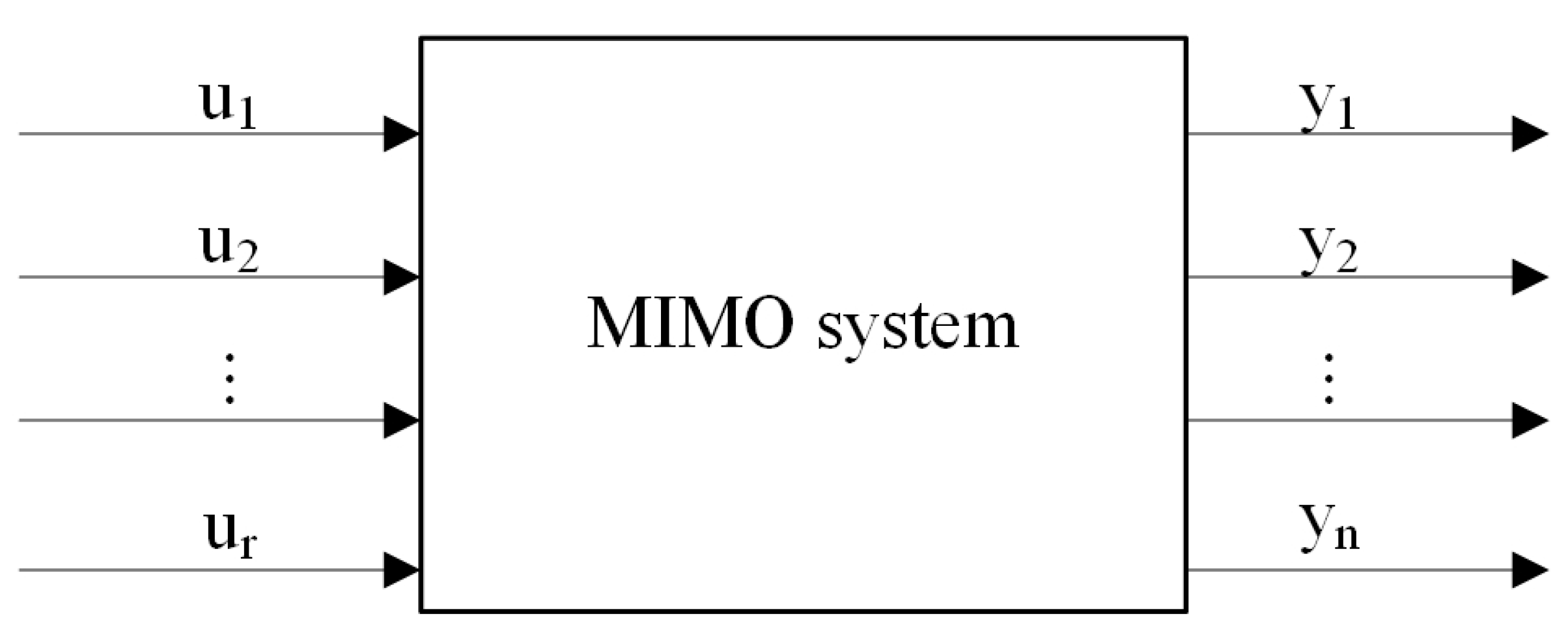
A linear multivariate system is shown in Figure 2. The state space equation description of a system is not unique and when the state of the state space equation model is not measurable, not only the parameters of the model but also the state of the model has to be estimated, which makes the identification more complicated, and it is more advantageous to use the transfer function matrix model to describe the identification system model.
The TFM model of the MIMO system is described as shown in Equation (9).
Y ( s ) = K 11 T 11 s + 1 K 1 r T 1 r s + 1 K n 1 T n 1 s + 1 K n r T n r s + 1 U ( s )
The parameter set K described in Equation (10) and the parameter set T described in Equation (11) are the sets of parameters that the system needs to recognize.
K = K 11 K 12 K i j K n r
T = T 11 T 12 T i j T n r
It is first necessary to discretize the discrete model (9) of the multivariate system into an impulse TFM model, as shown in Equation (12). In this paper, the discretization was carried out using the bilinear transformation method ( s = 2 T s 1 z 1 1 + z 1 ).
Y ( z ) = G 11 ( z 1 ) G 1 r ( z 1 ) G n 1 ( z 1 ) G n r ( z 1 ) U ( z )
Regarding the above-shown equation, the specific description of G i j ( z 1 ) is shown in Equation (13).
G i j ( z 1 ) = n i j , 0 + n i j , 1 z 1 + + n i j , q b i j z q b i j 1 + m i j , 1 z 1 + + m i j , p a i j z p a i j
where q b i j is the input signal order and p a i j is the output signal order.
Extracting the least common multiple of each row of the impulse TFM leads to Equation (14) and then converting the impulse TFM model to a difference equation model (Equation (15)).
1 + μ i , 1 z 1 + + μ i , n a i z n a i = ( 1 + + m i 1 , p a i 1 , i 1 z p a i 1 , i 1 ) ( 1 + + m i n , p a i n , i n z p a i n , i n )
y 1 ( k ) y n ( k ) = Y 1 ( k ) Y n ( k ) + U 1 ( k ) U n ( k )
where Y i ( k ) = μ i , 1 y i ( k 1 ) + + μ i , n a i y i ( k n a i ) , U i = λ i 1 , 0 u 1 ( k ) + + λ i 1 , q b i 1   u 1 ( k q b i 1 ) + + λ i r , 0 u r ( k ) + + λ i r , q b i r u r ( k q b i r ) .
The difference equation model parameters (Equation (16)) are first estimated and then the parameters K and T are inverted according to the discretization method used.
θ 1 = μ 1 , 1 μ 1 , n a 1 μ 2 , 1 μ 2 , n a 2 μ n , 1 μ n , n a n λ 11 , 0 λ 11 , q b 11 λ 1 r , 0 λ 1 r , q b 1 r λ 21 , 0 λ 21 , q b 21 λ 2 r , 0 λ 2 r , q b 2 r λ n 1 , 0 λ n 1 , q b n 1 λ n r , 0 λ n r , q b n r
Specifically, after determining the differential equation model, K and T are solved inversely according to the formulation of the bilinear transformation method. This can be achieved by using the d2c function in MATLAB.
For the MIMO system, we split the system into multiple Multi-Input and Single-Output (MISO) systems based on each output y i and study each MISO system.
Take the example of a two-input, two-output system (Equation (17)). It is discretized into a difference equation, which is described as Equation (18).
Y ( s ) = K 1 T 1 s + 1 K 2 T 2 s + 1 K 3 T 3 s + 1 K 4 T 4 s + 1 U ( s )
y 1 ( k ) y 2 ( k ) = μ 11 y 1 ( k 1 ) μ 12 y 1 ( k 2 ) μ 21 y 2 ( k 1 ) μ 22 y 2 ( k 2 ) + λ 11 u 1 ( k ) λ 12 u 1 ( k ) λ 13 u 1 ( k ) λ 21 u 2 ( k ) λ 22 u 2 ( k ) λ 23 u 2 ( k ) λ 31 u 1 ( k ) λ 32 u 1 ( k ) λ 33 u 1 ( k ) λ 41 u 2 ( k ) λ 42 u 2 ( k ) λ 43 u 2 ( k )
The inverse solution of K 1 ,   K 2 ,   K 3 ,   K 4 ,   T 1 ,   T 2 ,   T 3 ,   T 4 is performed according to the formulation of the bilinear transformation method, the expression of which is shown in Equation (19).
K 1 = 2 λ 11 λ 21 λ 22 K 2 = 2 λ 11 λ 21 λ 12 K 3 = 2 λ 31 λ 41 λ 42 K 4 = 2 λ 31 λ 41 λ 32 T 1 = 2 T s λ 21 T s λ 22 2 λ 22 T 2 = 2 T s λ 11 T s λ 12 2 λ 12 T 3 = 2 T s λ 41 T s λ 42 2 λ 42 T 4 = 2 T s λ 31 T s λ 32 2 λ 32
where T s is the system sampling time.
Parameter estimation for MIMO systems can be viewed as finding the relationship between the input vector X and multiple outputs y j . For each output y j , an SVR model is built to describe its relationship with the input vector X.
y j = f j ( X ) + μ j
For each output y j , we define an independent SVR optimization problem with the following objective function.
min w , b , ξ , ξ * 1 2 w j 2 + C i = 1 m ( ξ i j + ξ i * j ) s . t . w j , X i + μ j y j ε + ξ i j y j w j , X i μ j ε + ξ i * j ξ i j , ξ i * j 0
where w j is the weight vector of the corresponding SVR regression problem for each output signal y j .
By training the dataset X i , Y i , the output of each SVR model is trained individually.
After collecting the input and output signals, the dataset is constructed according to the data requirements of LIBSVM, including the label dataset and data dataset; for the regression problem, the label dataset is the independent variable dataset, and the data dataset is the dependent variable dataset. Parameter identification of multivariate systems based on SVR requires the construction of datasets as shown in Equations (22) and (23).
l a b e l = y i ( k 1 ) y i ( k 2 ) u 1 ( k ) u 1 ( k 1 ) u 1 ( k 2 ) u 2 ( k ) u 2 ( k 1 ) u 2 ( k 2 )
d a t a = [ y i ( k ) ]
The dataset was divided into training and test sets according to a certain ratio. The linear kernel function was selected based on the characteristics of the linear multivariate system. We then optimized the parameter C using the grid search method to achieve the best prediction result.
When the kernel function is a linear kernel function, the training system parameters, support vector weights, and support vectors can be used to find the discriminant parameters, as shown in Equation (24).
w = ( m o d e l . s v _ c o e f )     f u l l m o d e l . S V s
The specific process of SVR-based parameter identification is shown in Figure 3.

2.4. Unbiased and Error Convergence

For traditional estimation algorithms, such as the LS method, the most important properties of the method are unbiasedness and convergence of the error variance to zero.
SVR-based parameter estimation methods do not directly optimize for or guarantee unbiasedness and are more concerned with finding a model that strikes a balance between model complexity and prediction error. This bias facilitates the reduction of overfitting and improves the generalization ability of the model. Therefore, this paper considers the problem of parameter estimation under noise interference, and better results can be achieved by selecting SVR-based parameter estimation algorithms compared to traditional parameter estimation methods.
Whether the error variance of SVR-based parameter estimation methods can converge to zero depends on a number of factors, including the choice of model, the complexity of the feature space, the nature of the dataset, and the setting of the regularization parameters. Since the goal of SVR is to minimize the model complexity and prediction error, it is not possible to achieve complete convergence of the error variance to 0.
Although the complexity of the feature equations is performed to improve the accuracy of the parameter estimation, the model may be overfitted in this case. For the data studied in this paper, i.e., data containing noise, overfitting can lead to a parameter estimation problem that is heavily influenced by noise.

3. SVR Algorithm Using Stochastic Search and Bayesian Optimization

Stochastic search is a global search method that does not rely on gradient information, and it searches for optimal solutions by randomly sampling in the solution space. Unlike deterministic search algorithms, stochastic search does not rely on a priori knowledge and is insensitive to the choice of initial points, and thus exhibits unique robustness in dealing with discontinuous and nonconvex optimization problems. The core of the stochastic search algorithm is to utilize randomness to traverse the solution space, and it does not use any directed search strategy, which means that the decision at each step of the algorithm is independent of the previous step.
Its main process is as follows:
(1) Define the parameter space. Define the parameter space to be optimized according to the specific problem;
(2) Initial sampling. Randomly sample a set of initial parameter values from the parameter space according to a certain sampling method, such as uniform distribution, Gaussian distribution, and so on;
(3) Evaluation of objective function. Design the objective function according to the specific problem, and then calculate the corresponding objective function value for each set of parameter values;
(4) Update the best parameters. Record the best combination of parameters found and their corresponding objective function values;
(5) Iterative search. Repeat steps 2 to 4 until a predetermined number of iterations is reached or the stopping condition is met.
Compared with grid search, random search does not need to search for all parameter combinations, which greatly reduces the number of searches and time. Especially when the parameter space is very large, stochastic search can find the near-optimal parameter combinations with less computational resources and time cost.
Bayesian optimization is a global optimization method based on a probabilistic model, which searches for the optimal hyperparameters by constructing a probabilistic model of the objective function.
The core of Bayesian optimization lies in the use of a probabilistic model to model a black-box function and the use of this model to guide the process of finding the optimal solution. Probabilistic models use prior knowledge and observations to update the posterior distribution as a means of predicting the value of a function at points that have not yet been observed. The first step in constructing the model is to determine the prior distribution, which is usually based on assumptions about the prior knowledge of the problem.
The probabilistic model is then updated based on Bayes’ Law as new observations are obtained. Constructing a probabilistic model requires the selection of an appropriate family of probability distributions, which is commonly used as a Gaussian process (GP).
Its specific implementation process is as follows:
(1) Initial sampling. Randomly select some sampling points and calculate the corresponding objective function values;
(2) Construct an agent model of the objective function based on the initial sampling using the Gaussian process;
(3) Optimize the proxy model. Use the proxy model to predict the objective function values and uncertainties of the new parameter points. Calculate the acquisition function based on the above predictions to balance the trade-off between exploration and exploitation. In this case, exploration is the selection of points with higher uncertainty to discover new optimal points. Exploitation is conducted to select points with better expected objective function values to improve the optimal solution by utilizing existing information;
(4) Updating the agent model. The next parameter point is selected under the guidance of the acquisition function and its objective function value is calculated. Add the new data point to the existing data set to update the agent model;
(5) Iterative repetition. Repeat steps 3 and 4 to gradually reduce the parameter space and find the optimal parameters. The iterative process ends when the preset number of iterations or convergence conditions are reached.
Bayesian optimization predicts which parameter combinations are likely to lead to the best performance by constructing a probabilistic model of the objective function and then selects the parameters to be evaluated next based on this predictive model. This approach is more efficient compared to random and lattice searches and is able to find near-optimal parameters with fewer evaluations, especially if the objective function evaluation is costly. In addition, Bayesian optimization is an iterative optimization process where each step uses the information from the previous steps to improve the next search. This means that as the search proceeds, the optimization process becomes progressively more efficient and precise and is able to better focus on the possible regions of optimal parameters.
When the search space is large and the problem complexity is high, stochastic search covers the solution space well but lacks relevance and efficiency. On the other hand, Bayesian optimization methods provide good relevance and high efficiency, but require high prior knowledge of the problem and perform erratically in high-dimensional spaces. Combining the two aims to exploit the global search capability of stochastic search and the local search efficiency of Bayesian optimization.
The specific steps of the algorithm for combining the two are as follows:
(1) Define the parameter space. Define the range of values and distribution of each hyperparameter;
(2) Initial exploration using random search. Determine the number of initial searches according to the specific problem and computational resources, and collect the initial data points after a certain number of random searches;
(3) Construct a Bayesian optimization agent model. Construct the agent model of the objective function using the initial data points in step 2;
(4) Optimize the agent model. Use the agent model to predict the objective function values and uncertainties for the new parameter points. Calculate the acquisition function based on these predictions to balance the tradeoff between exploration and exploitation. In this case, exploration is the selection of points with higher uncertainty to discover new optimal points. Exploitation is conducted to select points with better expected objective function values to improve the optimal solution by utilizing existing information;
(5) Updating the agent model. The next parameter point is selected under the guidance of the acquisition function and its objective function value is calculated. Add the new data point to the existing data set to update the agent model;
(6) Iterative repetition. Repeat steps 4 and 5 to gradually reduce the parameter space and find the optimal parameters. The iterative process ends when the preset number of iterations or convergence conditions are reached.

4. Simulation and Experiment

4.1. Simulation

In order to demonstrate the effectiveness of the proposed method, a two-input single-output system was built for simulation. Its specific formula is shown in Equation (25).
Y ( s ) = 1 s + 1 3 5 s + 1 U ( s )
Bilinear discretization of the above transfer function matrix using MATLAB gives the impulse TFM as Equation (26).
0.04762 ( 1 + z 1 ) 1 0.9048 z 1 0.0297 ( 1 + z 1 ) 1 0.9802 z 1
The least common multiple is extracted for each row of the impulse TFM and transformed into the form of a difference equation, as described below:
y ( k ) = 1.885 y ( k 1 ) 0.8869 y ( k 2 ) + 0.04762 u 1 ( k ) + 0.00094 u 1 ( k 1 ) 0.046676 u 1 ( k 2 ) + 0.0297 u 2 ( k ) + 0.028 u 2 ( k 1 ) 0.05516 u 2 ( k 2 )
The parameters to be estimated for this system are shown in Equation (28).
a 1 = 1.885 a 2 = 0.8869 b 11 = 0.04762 b 12 = 0.00094 b 13 = 0.046676 b 21 = 0.0297 b 22 = 0.028 b 23 = 0.05516
The input signals 1 and 2 are both random signals, as shown in Figure 4.
The PC hardware configuration is a Windows 11 operating system, 16 g RAM, and the CPU is an Intel i7-1260p. The MATLAB version is R2018b.
The estimation of model parameters (see Equation (27)) was performed using the recursive least square (RLS), SVR, and RSBO-SVR methods in the presence of outliers or colored noise. The data were divided into a training set and a test set, where 2/3 is the training set and 1/3 is the test set.

4.1.1. Presence of Outliers

We assumed that there were two outliers y (100) = 100 and y (120) = −50 in the dataset. The recursive process of RLS identification is shown in Figure 5. The training and prediction results of SVR are shown in Figure 6. The training and prediction results of RSBO-SVR are shown in Figure 7. The specific recognition results and errors are shown in Table 2.
Using the above-estimated data, the values of the relevant parameters of the TFM are calculated according to Equation (19), and their specific values and errors from the set values are shown in Table 3.
From Figure 6, it can be seen that the outliers had a great influence on the parameter identification of RLS, which will make RLS completely invalid and unable to identify the correct parameters. On the contrary, SVR had a strong anti-interference ability to the outliers, and its parameter identification results still had a high correct rate, as shown in Table 2; the maximum error was 2.04%, and the maximum error of the transfer function matrix parameters obtained after the operation was 2.01%. The RSBO-SVR algorithm also had very good identification results; the maximum error of the parameters of the difference equation was not more than 2%, and the maximum error of the transfer function matrix parameters obtained after the operation was 2.01%. The maximum error of the transfer function matrix parameters was only 3.33%.

4.1.2. Colored Noise States

Assuming that the model of Equation (27) contains colored noise, the expression is shown in Equation (29).
e ( k ) = 1.5 e ( k 1 ) 0.7 e ( k 2 ) 0.1 e ( k 3 ) + 0.5 v ( k ) + 0.2 v ( k 1 )
where v ( k ) is a white noise signal with mean 0 and variance 1.
The training and prediction results of SVR and RSBO-SVR are shown in Figure 8 and Figure 9. The specific identification results and errors are shown in Table 4.
From the above-shown table, it can be seen that in most of the parameter identification results, SVR and RSBO-SVR performed closer to the set values than RLS, and the errors were generally lower than RLS. The maximum errors were 2.04% for SVR, 3.06% for RSBO-SVR, and 237.88% for RLS, which was more than 100 times higher than that of SVR, and more than 100 times higher than that of RSBO-SVR. The maximum error of RLS was 237.88%, which is more than 100 times greater than SVR and more than 70 times greater than RSBO-SVR. This shows that SVR and RSBO-SVR identify the parameters better than RLS in the presence of colored noise. The values of the relevant parameters of the transfer function matrix were calculated using the above-shown data, and the exact values and the errors with respect to the set values are shown in Table 5.
In the presence of colored noise in the system, although RLS could identify the relevant parameter values, the error was very large; as can be seen from the table above, the maximum error was 669.3% and the minimum error was more than 40%, and the model built by using this identification parameter could not accurately describe the system. In contrast, the maximum error of SVR was only 1.997%, and the maximum error of RSBO-SVR was only −3.5%, which could describe the relevant system better.
Both SVR and RSBO-SVR have good estimation accuracy, and we compared their estimation times, as shown in Table 6 below.
In the presence of outliers, the estimation time of RSBO-SVR decreased by 90.05% compared to SVR; in the presence of colored noise interference, the estimation time of RSBO-SVR decreased by 78.88% compared to SVR.

4.2. Experimental Verification

In order to verify the practical application of the algorithm, a water tank model was created. The diagram of the water tank model is shown in Figure 10.
Three systems need to be identified in the above-shown system. To explain in detail, the following is an example of Tank 1.
To identify Tank 1, we used a pressure sensor to obtain level information and a pump and ball valve to control the level. The current value of the pressure sensor was obtained, and the current values of the input pump and ball valve were used as identification data.
The input data and output data are shown in Figure 11. The complete data are shown in Appendix A. Parameter estimation was carried out using SVR and RSBO-SVR algorithms and the training and prediction process is shown in Figure 12 and Figure 13.
The final recognized model of SVR is shown in Equation (30). The recognized model of RSBO-SVR is shown in Equation (31).
y ( k ) = 0.8107 y ( k 1 ) + 0.1717 y ( k 2 ) 0.0074 u 1 ( k 2 ) 0.0055 u 1 ( k 3 ) 0.0222 u 2 ( k 2 ) + 0.0015 u 2 ( k 3 ) + 0.4492
y ( k ) = 0.7998 y ( k 1 ) + 0.2056 y ( k 2 ) 0.0077 u 1 ( k 2 ) 0.0053 u 1 ( k 3 ) 0.0219 u 2 ( k 2 ) + 0.0015 u 2 ( k 3 ) + 0.4001
To verify the accuracy of the estimated model, the same input signals were given to the estimated model and the actual system. The output signals and errors of the two systems are shown in Figure 14 and Figure 15.
The error between the estimated output signal and the actual output signal of the SVR algorithm was effectively controlled within ±1.5%. The maximum error between the estimated output signal and the actual output signal of the RSBO-SVR algorithm did not exceed 3%. This indicates that the accuracy of the estimation process of SVR and RSBO-SVR was very high. The estimation time of SVR was 4085 s and the estimation time of RSBO-SVR was 25 s. The estimation accuracy of RSBO-SVR decreased in comparison with SVR, but its estimation speed improved dramatically, being 99.38% faster when compared with SVR.

5. Conclusions

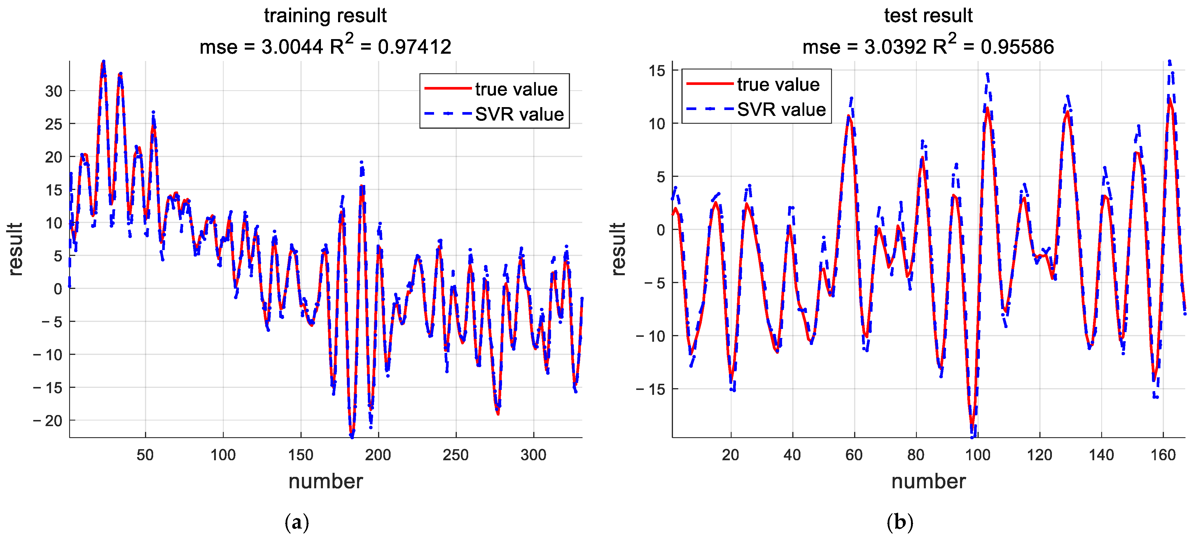
In this study, we investigated the performance of SVR and RSBO-SVR algorithms for parameter identification in multivariate systems, including challenging conditions such as common outliers and colored noise disturbances. The results showed that both the RSBO-SVR and SVR algorithms utilize the structural risk minimization principle and the L2 regularization term to effectively reduce the complexity of the model while maintaining robustness to noise disturbances. Specifically, the use of the maximum margin strategy and insensitive loss function enabled the model to effectively resist noise and outliers.
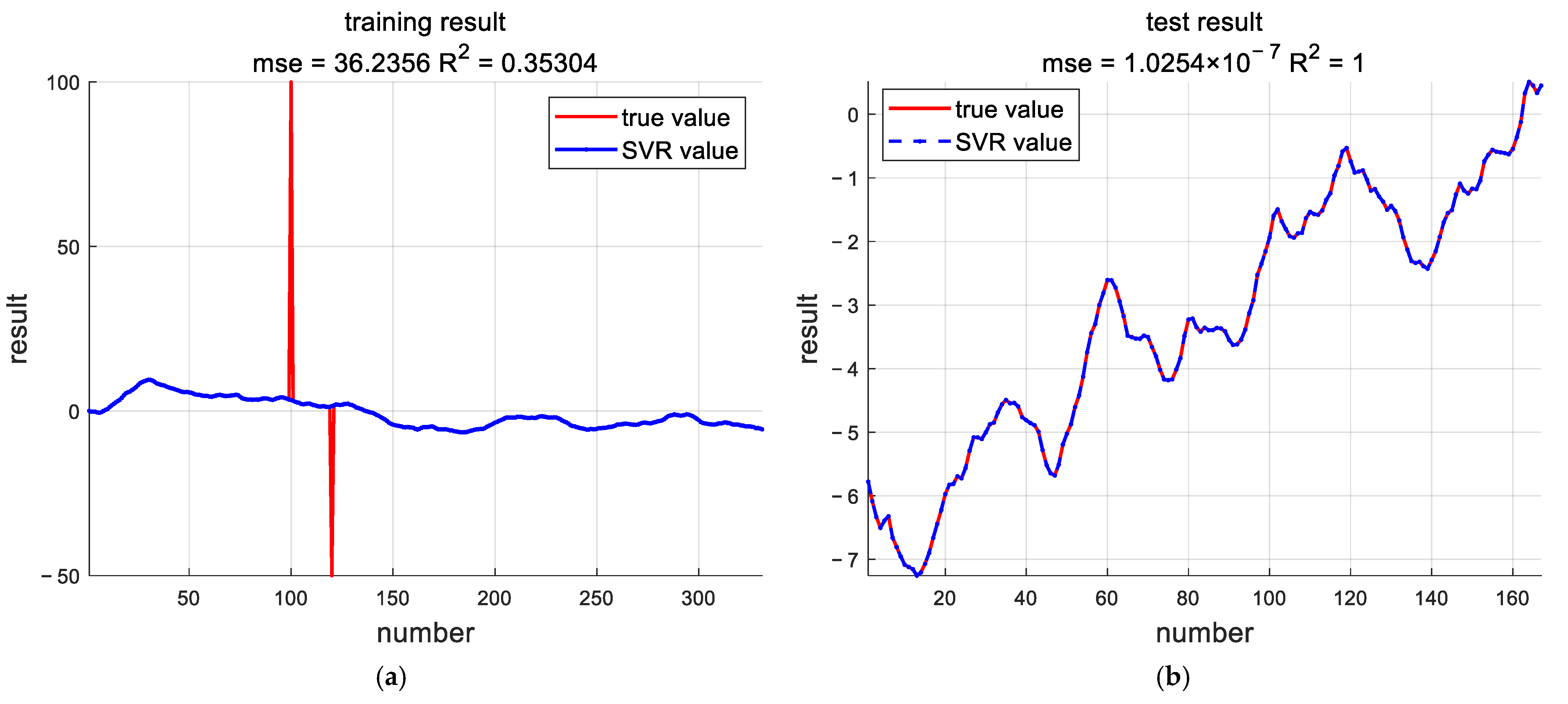
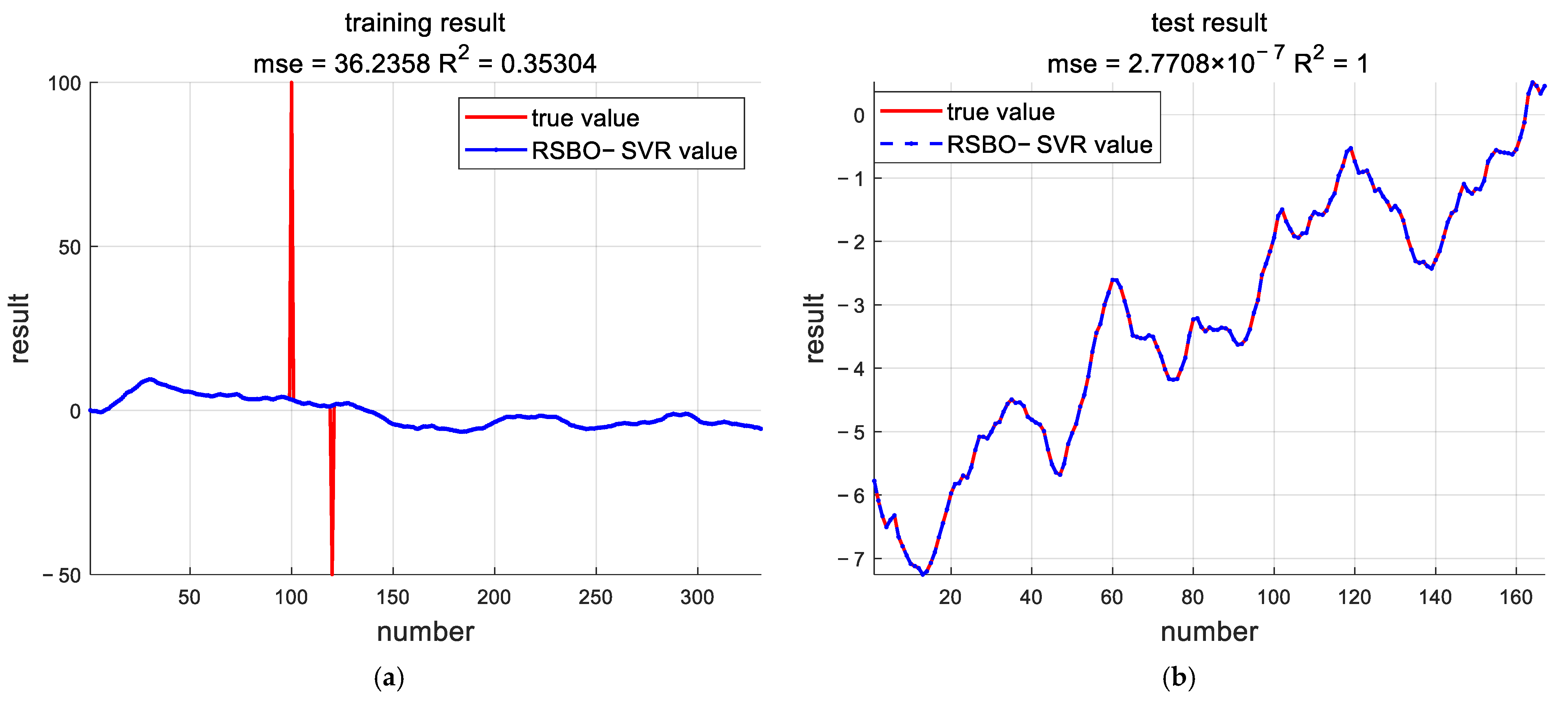
For parameter identification of multivariate systems, the RLS algorithm was completely ineffective when there were outliers in the collected input and output data. The SVR algorithm and RSBO-SVR algorithm, however, still had high identification accuracy under the same conditions. In addition, in order to solve the problem of the long optimization time of SVR parameters, the RSBO-SVR algorithm combining random search and Bayesian optimization is proposed. When the system contains colored noise, RLS could identify the parameters, but the error was very large, and the identified system could not correctly reflect the system characteristics. In contrast, color noise had less of an effect on the SVR and RSBO-SVR algorithms. Compared with SVR, RSBO-SVR had a faster estimation speed.
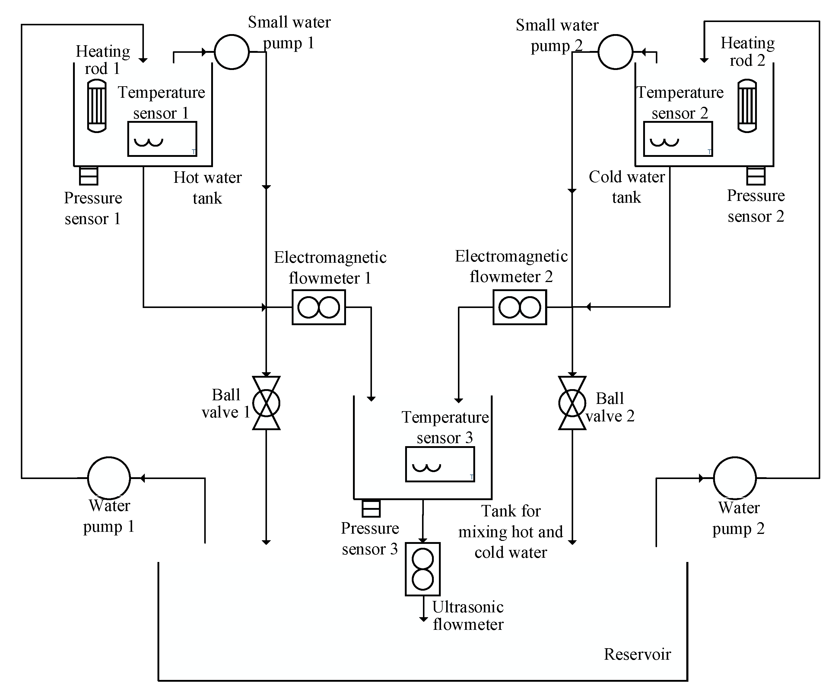
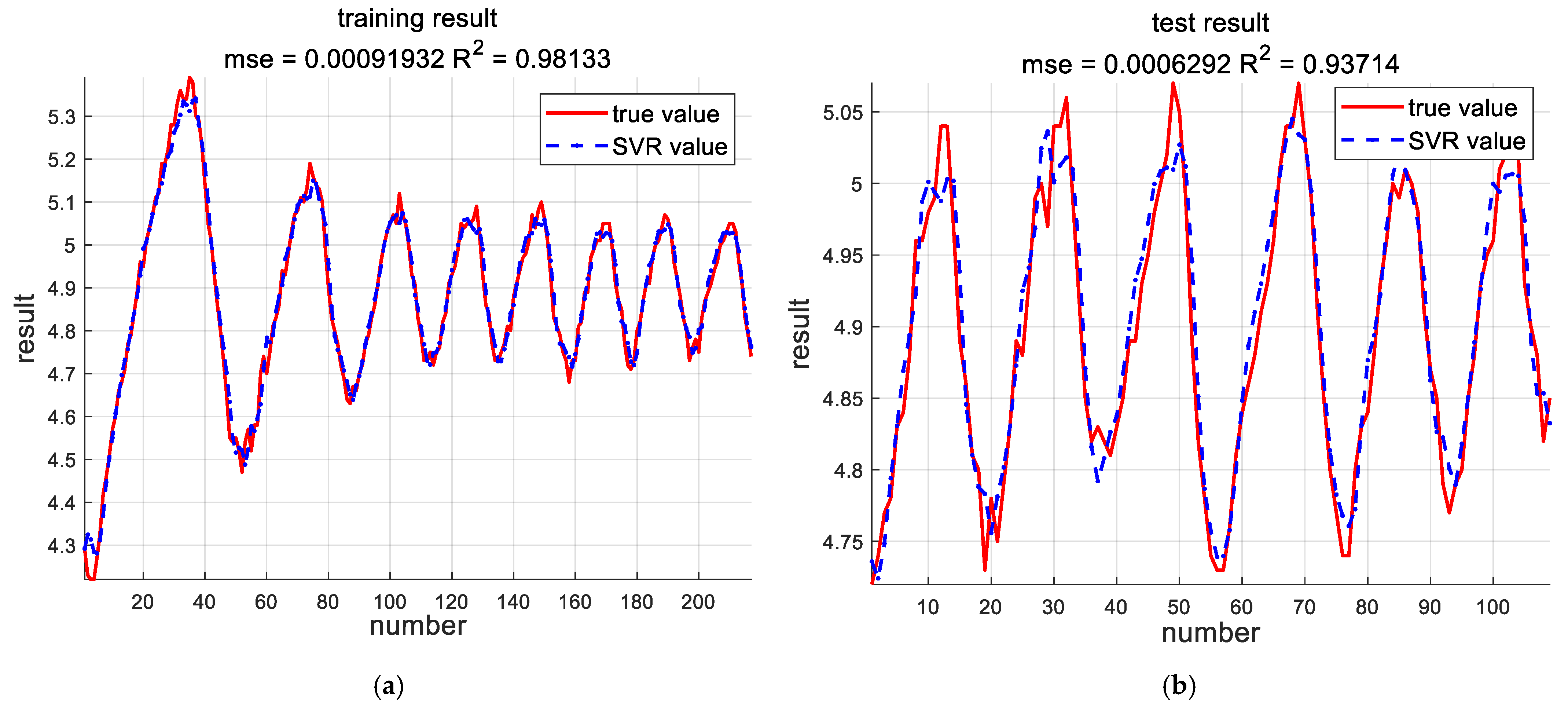
In addition, the tank experiments prove that these algorithms can be applied to the identification of real systems; the maximum output error between the estimated model and the actual model was only 1.5% for the SVR algorithm, and the maximum output error between the estimated model and the actual model was not more than 3% for the RSBO-SVR algorithm. Although the accuracy is lower than SVR, it still meets the requirements of industrial production. Compared with SVR, the estimation time of RSBO-SVR was 99.38% shorter.

6. Limitation of Study

There are three main limitations in this study: first, the parameter estimation model was constructed based on a linear multivariate system; although fast and accurate parameter identification can be achieved by the proposed method, it may generate modeling bias for an actual engineering system with strong nonlinear coupling characteristics. Second, although the SVR-based parameter estimation algorithm balances the model complexity and prediction error via L2 regularization, its loss function design does not impose explicit constraints on the unbiasedness of parameter estimation. Third, the current framework does not introduce a compensation mechanism for non-minimum phase zeros and time lag links, which may widen the phase margin prediction error for hydraulic servo systems with significant inverted response characteristics or process control objects with transmission delays of more than 40% of the sampling period, potentially affecting their applicability in specific industrial scenarios. These limitations point the way to improvements in subsequent research, including the introduction of a nonlinear model predictive control framework [46,47], the incorporation of Bayesian regularization constraints [48], and the embedding of Padé time-lag approximation modules [49].

Author Contributions

Conceptualization, J.Z. and X.J.; data curation, J.Z.; funding acquisition, X.J.; methodology, J.Z. and X.J.; software, J.Z.; writing—original draft, J.Z.; writing—review and editing, J.Z. and X.J. All authors have read and agreed to the published version of the manuscript.

Funding

This paper was funded by the National Natural Science Foundation of China (62063026) and also supported by the Natural Science Foundation of Inner Mongolia (2024LHMS06009).

Data Availability Statement

The original contributions presented in the study are included in the article, further inquiries can be directed to the corresponding author.

Conflicts of Interest

The authors declare no conflicts of interest.

Appendix A

Table A1. The data of tank 1.
Time/sWater Pump Output/mABall Valve/mAPressure Sensor Output/mA
01954.25
31954.22
51954.29
71954.23
91954.22
111954.22
131954.27
151954.33
181954.42
201954.46
221954.51
241954.57
261954.6
281954.66
301954.68
321954.71
351954.77
371954.79
391954.84
411954.89
431954.96
4518.495.514.95
4717.996.015.01
5017.476.535.04
5216.957.055.07
5416.427.585.11
5615.878.135.12
5815.328.685.19
6014.749.265.19
6214.169.845.22
6513.5510.455.28
6712.9311.075.28
6912.2911.715.33
7111.6312.385.36
7310.9313.075.34
7510.2213.785.34
779.4914.515.39
798.7315.275.38
827.9416.065.3
847.1416.865.29
866.3217.685.23
885.518.55.14
905195.05
925195.01
945194.93
965.8118.194.86
996.6317.374.8
1017.4616.544.73
1038.3115.694.65
1059.1914.814.55
10710.0913.914.54
10911.0212.984.55
11111.9612.044.52
11412.9211.084.47
11613.9110.094.54
11814.929.084.57
12015.958.054.52
12217.016.994.58
12418.085.924.58
1261954.7
1281954.74
1311954.7
1331954.75
1351954.81
1371954.83
1391954.86
1411954.94
1431954.93
1461954.98
14817.896.115.03
15016.777.235.07
15215.658.355.08
15414.529.485.11
15613.3810.625.1
15812.2411.765.13
16011.0912.915.19
1639.9114.095.16
1658.7315.275.14
1677.5416.465.13
1696.3317.675.1
1715.1118.894.99
1735194.9
1756.2117.794.83
1787.4316.574.8
1808.6615.344.77
1829.8914.114.72
18411.1412.864.69
18612.4111.594.64
18813.6910.314.63
1901594.67
19216.327.684.66
19517.666.344.7
1971954.72
1991954.77
2011954.79
2031954.83
2051954.86
2071954.91
2101954.96
21217.646.365
21416.287.725.03
21614.919.095.05
21813.5410.465.07
22012.1611.845.05
22210.7913.215.12
2249.414.65.07
2278165.05
2296.5917.415
2315.1818.824.93
2336.5817.424.91
2357.9916.014.83
2379.4114.594.79
23910.8413.164.73
24112.2811.724.73
24413.7310.274.75
24615.198.814.72
24816.677.334.75
25018.175.834.76
2521954.82
2541954.84
2561954.91
2581954.93
2611954.95
26317.56.54.99
2651685.05
26714.59.55.04
26912.9911.015.05
27111.4812.525.05
2739.9714.035.06
2768.4515.555.09
2786.917.15.02
2805.3618.644.93
2826.917.14.86
2848.4515.554.84
2869.9914.014.77
28811.5512.454.73
29013.1310.874.73
29314.719.294.75
29516.317.694.77
29717.936.074.81
2991954.8
3011954.88
3031954.91
3051954.94
3071954.97
31017.386.624.98
31215.778.235.01
31414.159.855.07
31612.5211.485.04
31810.913.15.08
3209.2714.735.1
3227.6116.395.06
3245.9518.055.01
3275194.93
3296.6617.344.83
3318.3315.674.81
33310144.79
33511.6812.324.75
33713.3710.634.73
33915.088.924.68
34216.817.194.73
34418.555.454.73
3461954.81
3481954.82
3501954.89
3521954.89
3541954.97
35617.256.754.99
35915.58.55.01
36113.7510.255.01
36312125.05
36510.2513.755.05
3678.4815.525.05
3696.717.34.99
3715194.91
3746.7817.224.87
3768.5715.434.85
37810.3513.654.77
38012.1511.854.72
38213.9610.044.71
38415.88.24.73
38617.656.354.8
3881954.82
3911954.87
3931954.91
3951954.91
3971954.97
39917.146.865
40115.298.715.01
40313.4410.565.04
40511.5812.425.07
4089.7214.285.06
4107.8416.165.03
4125.9618.044.96
4145194.92
4166.8817.124.88
4188.7715.234.83
42010.6613.344.8
42212.5511.454.73
42514.469.544.76
42716.397.614.78
42918.335.674.75
4311954.83
4331954.87
4351954.89
4371954.91
4391954.94
4421954.96
44417.056.955
44615.18.95.01
44813.1510.855.03
45011.212.85.05
4529.2514.755.05
4547.2816.725.03
4565.318.74.96
4595194.91
4616.9817.024.83
4638.9715.034.79
46510.9713.034.74
46712.9811.024.72
4691594.74
47117.036.974.77
4741954.78
4761954.83
4781954.84
4801954.88
4821954.96
48416.957.054.96
48614.99.14.98
48812.8511.154.99
49110.8113.195.04
4938.7515.255.04
4956.6917.314.97
4975194.89
4997.0816.924.86
5019.1614.844.81
50311.2512.754.8
50613.3310.674.73
50815.458.554.78
51017.576.434.75
5121954.79
5141954.83
5161954.89
5181954.88
5201954.93
5231954.99
52516.857.155
52714.719.294.97
52912.5711.435.04
53110.4313.575.04
5338.2915.715.06
5356.1217.884.99
5385194.92
5407.1716.834.85
5429.3414.664.82
54411.5212.484.83
54613.6910.314.82
54815.878.134.81
55018.075.934.83
5521954.85
5551954.89
5571954.89
5591954.93
5611954.95
56316.797.214.98
56514.599.415
56712.3811.625.02
56910.1813.825.07
5727.9616.045.05
5745.7218.284.99
5765194.89
5787.2416.764.82
5809.4914.514.78
58211.7512.254.74
58414.019.994.73
58716.297.714.73
58918.595.414.76
5911954.81
5931954.84
5951954.86
5971954.88
5991954.91
6011954.93
6041954.96
60616.697.315.01
60814.389.635.04
61012.0611.945.04
6129.7514.255.07
6147.4216.585.03
6165.0818.924.99
6185194.91
6217.3416.664.85
6239.6914.314.8
62512.0411.964.77
62714.49.64.74
62916.797.214.74
6311954.8
6331954.83
6351954.84
6381954.88
6401954.93
6421954.96
64416.597.415
64614.199.814.99
64811.812.25.01
6509.414.65
6527174.98
6555194.91
6577.4216.584.87
6599.8414.164.85
66112.2611.744.79
66314.699.314.77
66517.146.864.79
6671954.8
6701954.85
6721954.88
6741954.93
6761954.95
67816.547.464.96
68014.089.925.01
68211.6212.385.02
6849.1614.845.05
6876.6817.325.02
6895194.93
6917.4816.524.9
6939.9614.044.88
69512.4511.554.82

References

  1. Young, P.C. Parallel Processes in Hydrology and Water Quality: A Unified Time-series Approach. J. Inst. Water Environ. Manag. 1992, 6, 598–612. [Google Scholar] [CrossRef]
  2. Johnson, M.L.; Faunt, L.M. Parameter estimation by least-squares methods. Methods Enzymol. 1992, 210, 1–37. [Google Scholar] [CrossRef] [PubMed]
  3. Chen, B.; Xu, Y.; Shrivastava, A. Fast and Accurate Stochastic Gradient Estimation. In Proceedings of the Neural Information Processing Systems, Vancouver, BC, Canada, 8–14 December 2019. [Google Scholar]
  4. Meng, D. Recursive Least Squares and Multi-innovation Gradient Estimation Algorithms for Bilinear Stochastic Systems. Circuits Syst. Signal Process. CSSP 2017, 36, 1052–1065. [Google Scholar] [CrossRef]
  5. Gibson, S.; Wills, A.; Ninness, B. Maximum-likelihood parameter estimation of bilinear systems. IEEE Trans. Autom. Control AC 2005, 50, 1581–1596. [Google Scholar] [CrossRef]
  6. Li, J.; Ding, F.; Hua, L. Maximum likelihood Newton recursive and the Newton iterative estimation algorithms for Hammerstein CARAR systems. Nonlinear Dyn. 2013, 75, 235–245. [Google Scholar] [CrossRef]
  7. Wang, H.; Memon, F.H.; Wang, X.; Li, X.; Zhao, N.; Dev, K. Machine learning-enabled MIMO-FBMC communication channel parameter estimation in IIoT: A distributed CS approach. Digit. Commun. Netw. Engl. Ed. 2023, 9, 306–312. [Google Scholar] [CrossRef]
  8. Cerone, V.; Razza, V.; Regruto, D. Set-membership errors-in-variables identification of MIMO linear systems. Automatica 2018, 90, 25–37. [Google Scholar] [CrossRef]
  9. Liu, L.; Wang, Y.; Wang, C.; Ding, F.; Hayat, T. Maximum likelihood recursive least squares estimation for multivariate equation-error ARMA systems. J. Frankl. Inst. 2018, 355, 7609–7625. [Google Scholar] [CrossRef]
  10. Cecilio, I.M.; Ottewill, J.R.; Fretheim, H.; Thornhill, N.F. Multivariate Detection of Transient Disturbances for Uni- and Multirate Systems. IEEE Trans. Control Syst. Technol. 2014, 23, 1477–1493. [Google Scholar] [CrossRef]
  11. Kulikova, M.V.; Tsyganova, J.V.; Kulikov, G.Y. UD-Based Pairwise and MIMO Kalman-Like Filtering for Estimation of Econometric Model Structures. IEEE Trans. Control Syst. Technol. 2020, 65, 4472–4479. [Google Scholar] [CrossRef]
  12. Weijtjens, W.; De Sitter, G.; Devriendt, C.; Guillaume, P. Operational modal parameter estimation of MIMO systems using transmissibility functions. Automatica 2014, 50, 559–564. [Google Scholar] [CrossRef]
  13. Astrm, K.J.; Murray, R.M. Feedback Systems: An Introduction for Scientists and Engineers; Princeton University Press: Princeton, NJ, USA, 2008. [Google Scholar]
  14. Stoica, P.; Jansson, M. MIMO System Identification: State-Space and Subspace Approximations versus Transfer Function and Instrumental Variables. IEEE Trans. Signal Process. 2000, 48, 3087–3099. [Google Scholar] [CrossRef]
  15. Gu, Y.; Ding, F.; Li, J. States based iterative parameter estimation for a state space model with multi-state delays using decomposition. Signal Process. 2015, 106, 294–300. [Google Scholar] [CrossRef]
  16. Gre, S.; Dhlerm, M.; Jacobsen, N.J.; Mevel, L. Uncertainty quantification of input matrices and transfer function in input/output subspace system identification. Mech. Syst. Signal Process. 2022, 167, 108581. [Google Scholar] [CrossRef]
  17. Wang, J.; Wang, H.W.; Xia, H. Subspace-based closed-loop identification of multi-rate control system. Inf. Control 2014, 43, 6. [Google Scholar]
  18. You, J.; Huang, C.; Zhang, H. Combined invariant subspace & frequency-domain subspace method for identification of discrete-time MIMO linear systems. Syst. Control Lett. 2023, 181, 105641. [Google Scholar] [CrossRef]
  19. Liu, Y.J.; Ding, F. Coupled stochastic gradient algorithm and performance analysis for multivariable systems. Control Decis. 2016, 31, 1487–1492. [Google Scholar] [CrossRef]
  20. Pearson, A.; Chin, Y. Identification of MIMO systems with partially decoupled parameters. IEEE Trans. Autom. Control 1979, 24, 599–604. [Google Scholar] [CrossRef]
  21. Li, J.; Ruiz-Sandoval, M.; Spencer, B.F., Jr.; Elnashai, A.S. Parametric time-domain identification of multiple-input systems using decoupled output signals. Earthq. Eng. Struct. Dyn. 2014, 43, 1307–1324. [Google Scholar] [CrossRef]
  22. Kord, S.; Taghikhany, T. Parametric system identification of large-scale structure using decoupled synchronized signals. Struct. Des. Tall Spec. Build. 2022, 31, e1915. [Google Scholar] [CrossRef]
  23. Liang, X.Z.; Huang, Z.Y.; Ai, F.; Yuan, Z.; Wang, J. Dynamic modeling and parameterization of transfer function of plate-fin heat exchanger. J. Beijing Univ. Aeronaut. Astronaut. 2024, 50, 154–162. [Google Scholar]
  24. Pan, J.; Zhang, H.; Guo, S.L.Y. Multivariable CAR-like System Identification with Multi-innovation Gradient and Least Squares Algorithms. Int. J. Control Autom. Syst. 2023, 21, 1455–1464. [Google Scholar] [CrossRef]
  25. Vapnik, V. The Natural of Statistical Learning Theory; Springer Science & Business Media: New York, NY, USA, 1995. [Google Scholar] [CrossRef]
  26. Liu, Y.; Li, Y.; Duan, Z.; Wu, H. Study of aircraft system identification based on support vector machine. Aviat. Sci. Technol. 2019, 30, 68–72. [Google Scholar]
  27. Liu, Y.; Pi, D.; Cheng, Q. Ensemble kernel method: SVM classification based on game theory. J. Syst. Eng. Electron. 2016, 27, 251–259. [Google Scholar] [CrossRef]
  28. Keerthi, S.S.; Shevade, S.K. A fast iterative nearest point algorithm for support vector machine classifier design. IEEE Trans. Neural Netw. 2000, 11, 124–136. [Google Scholar] [CrossRef]
  29. Shashua, A.A. On the Relationship Between the Support Vector Machine for Classification and Sparsified Fisher’s Linear Discriminant. Neural Process. Lett. 1999, 9, 129–139. [Google Scholar] [CrossRef]
  30. Bredensteiner, E.J.; Bennett, K.P. Multicategory Classification by Support Vector Machines. Comput. Optim. Appl. 1999, 12, 53–79. [Google Scholar] [CrossRef]
  31. Yanwei, H.; Tihua, W.; Jingyi, Z. System identification and simulation by regressive support vector machine. Comput. Simul. 2004, 21, 4. [Google Scholar]
  32. Castro-Garcia, R.; Agudelo, O.M.; Johan, A.K. Impulse response constrained LS-SVM modeling for MIMO Hammerstein system identification. Int. J. Control 2019, 92, 908–925. [Google Scholar] [CrossRef]
  33. Li, J.; Ding, F. Maximum likelihood stochastic gradient estimation for Hammerstein systems with colored noise based on the key term separation technique. Comput. Math. Appl. 2011, 62, 4170–4177. [Google Scholar] [CrossRef]
  34. Shutong, L.; Yan, J.; Anning, J. Parameter Estimation Method for Generalized Time-varying Systems with Colored Noise Based on the Hierarchical Principle. Int. J. Control. Autom. Syst. 2024, 22, 548–559. [Google Scholar] [CrossRef]
  35. Liu, S.; Wang, Y.; Ding, F.; Alsaedi, A.; Hayat, T. Joint iterative state and parameter estimation for bilinear systems with autoregressive noises via the data filtering. ISA Trans. 2024, 147, 337–349. [Google Scholar] [CrossRef] [PubMed]
  36. Kuo, S.M.; Morgan, D.R. Active noise control: A tutorial review. Proc. IEEE 1999, 87, 943–973. [Google Scholar] [CrossRef]
  37. Shi, Y.; Yuan, Y.; Luo, B.; Li, F.; Xu, X.; Yang, C. Data-Driven Plant-Model Mismatch Detection for Closed-Loop LPV System Based on Instrumental Variable Using Sum-of-Norms Regularization. IEEE Trans. Instrum. Meas. 2024, 73, 3001612. [Google Scholar] [CrossRef]
  38. Yue, Z.; Guiming, L. A recursive algorithm for parameter identification of colored noise interference systems. J. Tsinghua Univ. (Nat. Sci. Ed.) 2009, 49, 135–137+141. [Google Scholar] [CrossRef]
  39. Xu, L.; Ding, F.; Zhang, X.; Zhu, Q. Novel parameter estimation method for the systems with colored noises by using the filtering identification idea. Syst. Control Lett. 2024, 186, 105774. [Google Scholar] [CrossRef]
  40. Zhang, Y.; Li, Q. A Regressive Convolution Neural Network and Support Vector Regression Model for Electricity Consumption Forecasting. In Advances in Information and Communication: Proceedings of the 2019 Future of Information and Communication Conference (FICC), San Francisco, CA, USA, 14–15 March 2019; Springer: Cham, Switzerland, 2020. [Google Scholar]
  41. Lin, K.C.; Chien, H.Y. CSO-based feature selection and parameter optimization for support vector machine. In Proceedings of the 2009 Joint Conferences on Pervasive Computing (JCPC), Tamsui, Taiwan, 3–5 December 2009; IEEE: New York, NY, USA, 2010. [Google Scholar] [CrossRef]
  42. Gao, Z.; Li, L. Adaptive optimization of cutting parameters in milling industry considering dynamic tool wear in intelligent manufacturing driven by reinforcement learning. Int. J. Adv. Manuf. Technol. 2024, 133, 4751–4760. [Google Scholar] [CrossRef]
  43. Der, O.; Ordu, M.; Basar, G. Optimization of cutting parameters in manufacturing of polymeric materials for flexible two-phase thermal management systems. Mater. Test. 2024, 66, 1700–1719. [Google Scholar] [CrossRef]
  44. Smola, A.J.; Schölkopf, B. A tutorial on support vector regression. Stat. Comput. 2004, 14, 199–222. [Google Scholar] [CrossRef]
  45. Schölkopf, B.; Smola, A.J. Learning with Kernels; MIT Press: Cambridge, MA, USA, 2002. [Google Scholar]
  46. Baydokhty, M.E.; Zare, A.; Balochian, S. Performance of optimal hierarchical type 2 fuzzy controller for load–frequency system with production rate limitation and governor dead band. Alex. Eng. J. 2016, 55, 379–397. [Google Scholar] [CrossRef]
  47. Namadchian, Z.; Zare, A.; Namadchian, A. Stability Analysis of Nonlinear Dynamic Systems by Nonlinear Takagi-Sugeno-Kang Fuzzy Systems. J. Dyn. Syst. Meas. Control-Trans. ASME 2014, 136, 021019. [Google Scholar] [CrossRef]
  48. Byrd, M.; Nghiem, L.H.; McGee, M. Bayesian regularization of Gaussian graphical models with measurement error. Comput. Stat. Data Anal. 2021, 156, 107085. [Google Scholar] [CrossRef]
  49. Hussein, A.A.; Hajj, M.R.; Elkholy, S.M.; ELbayoumi, G.M. Dynamic Stability of Hingeless Rotor Blade in Hover Using Pade Approximations. AIAA J. 2016, 54, 1769–1777. [Google Scholar] [CrossRef]
Figure 1. Schematic diagram of the SVR principle. (The circles are the data points that need to be fitted).
Processes 13 00773 g001
Figure 2. MIMO system architecture diagram.
Processes 13 00773 g002
Figure 3. The flowchart of SVR.
Processes 13 00773 g003
Figure 4. Input signals.
Processes 13 00773 g004
Figure 5. Diagrams of the RLS identification process of a and b (with outliers). (a) The identification process of parameter a; (b) The identification process of parameter b.
Processes 13 00773 g005
Figure 6. The training and test fit plots of SVR (with outliers). (a) The training process of SVR; (b) The test process of SVR.
Processes 13 00773 g006
Figure 7. The training and test fit plots of RSBO-SVR (with outliers). (a) The training process of RSBO-SVR; (b) The test process of RSBO-SVR.
Processes 13 00773 g007
Figure 8. The training and test fit plots of SVR (with colored noise). (a) The training process of SVR; (b) The test process of SVR.
Processes 13 00773 g008
Figure 9. The training and test fit plots of RSBO-SVR (with colored noise). (a) The training process of RSBO-SVR; (b) The test process of RSBO-SVR.
Processes 13 00773 g009
Figure 10. The model diagram of the real water tank.
Processes 13 00773 g010
Figure 11. The real input and output signals of tank 1. (a) The input signals; (b) The output signal.
Processes 13 00773 g011
Figure 12. The training and test fit plots of tank 1 using SVR. (a) The training process of SVR; (b) The test process of SVR.
Processes 13 00773 g012
Figure 13. The training and test fit plots of tank 1 using RSBO-SVR. (a) The training process of RSBO-SVR; (b) The test process of RSBO-SVR.
Processes 13 00773 g013
Figure 14. (a) The output signals of the real and the estimated system (SVR); (b) the error between the real and estimated output (SVR).
Processes 13 00773 g014
Figure 15. (a) The output signals of the real and the estimated system (RSBO-SVR); (b) the error between the real and estimated output (RSBO-SVR).
Processes 13 00773 g015
Table 1. The kernel functions and their calculation formulas.
Kernel FunctionCalculation Formula
Linear kernel function K ( x i , x j ) = x i T x j
Polynomial kernel function K ( x i , x j ) = ( γ x i T x j + b ) d
RBF K ( x i , x j ) = exp γ x i x j 2
Sigmoid kernel function K ( x i , x j ) = tanh ( γ x i T x j + b )
Table 2. The identification results and errors of SVR and RSBO-SVR (with outliers).
ParametersSetpointsSVRRSBO-SVRSVR ErrorRSBO-SVR Error
a 1 1.8851.8854671.8855830.02%0.03%
a 2 −0.8869−0.887002−0.885850.01%−0.12%
b 11 0.047620.0473060.047903−0.66%0.59%
b 12 0.000940.0009370.000935−0.32%−0.53%
b 13 −0.046676−0.047586−0.0469771.95%0.64%
b 21 0.02970.0303070.0302542.04%1.87%
b 22 0.00280.0028510.0028311.82%1.11%
b 23 −0.05516−0.054962−0.0554611−0.36%0.55%
Table 3. Estimation results for the parameters of the transfer function matrix (with outliers).
ParametersSetpointsSVRRSBO-SVRSVR ErrorRSBO-SVR Error
K 1 11.0057541.0238480.58%2.38%
K 2 33.0601983.1000162.01%3.33%
T 1 11.0130311.0186681.30%1.87%
T 2 54.9986665.073316−0.03%1.47%
Table 4. The identification results and errors of RLS, SVR, and RSBO-SVR (with colored noise).
ParametersSetpointsRLSSVRRSBO-SVRRLS ErrorSVR ErrorRSBO-SVR Error
a 1 1.8851.71991.8854671.885395−8.76%0.02%0.02%
a 2 −0.8869−0.8937−0.887002−0.886870.77%0.01%0.00%
b 11 0.047620.16090.0473060.047441237.88%−0.66%−0.38%
b 12 0.000940.0005340.0009370.000942−43.19%−0.32%0.21%
b 13 −0.046676−0.0043−0.047586−0.048103−90.79%1.95%3.06%
b 21 0.02970.03830.0303070.02897628.96%2.04%−2.44%
b 22 0.00280.00870.0028510.002849210.71%1.82%1.75%
b 23 −0.05516−0.0092−0.054962−0.055081−83.32%−0.36%−0.14%
Table 5. Estimation results for the parameters of the transfer function matrix (with colored noise).
ParametersSetpointsRLSSVRRSBO-SVRRLS ErrorSVR ErrorRSBO-SVR Error
K 1 11.4171.00590.96500641.7%0.59%−3.50%
K 2 323.083.05992.918578669.3%1.997%−2.71%
T 1 10.391.0130.967059−61%1.3%−3.29%
T 2 530.084.99874.9862501.6%−0.026%−0.28%
Table 6. Estimated times for SVR and RSBO-SVR.
StateSVRRSBO-SVR
With outliers201 s20 s
With colored noise251 s53 s
Disclaimer/Publisher’s Note: The statements, opinions and data contained in all publications are solely those of the individual author(s) and contributor(s) and not of MDPI and/or the editor(s). MDPI and/or the editor(s) disclaim responsibility for any injury to people or property resulting from any ideas, methods, instructions or products referred to in the content.

