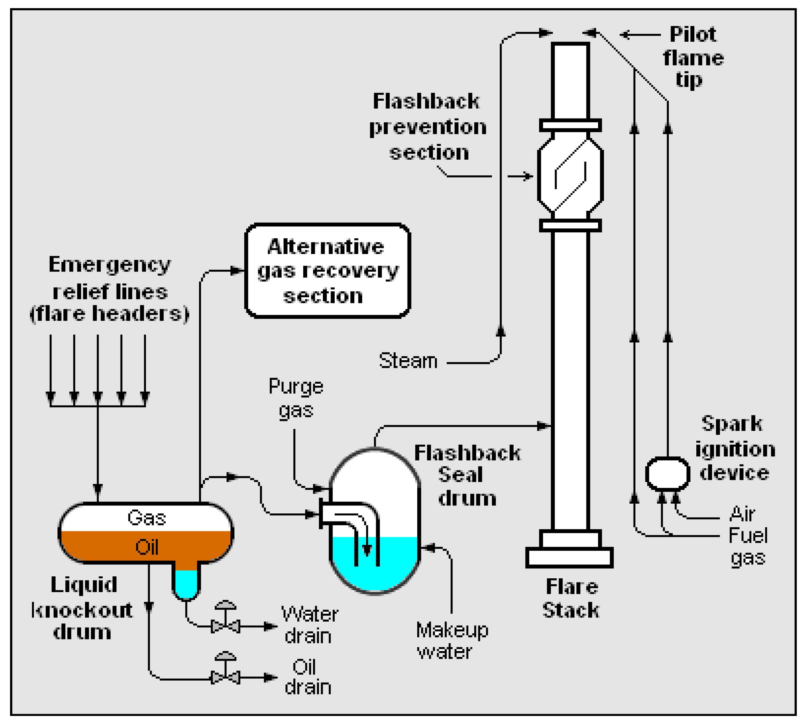
Figure 1.
Typical gas flare system [
3].
Figure 1.
Typical gas flare system [
3].
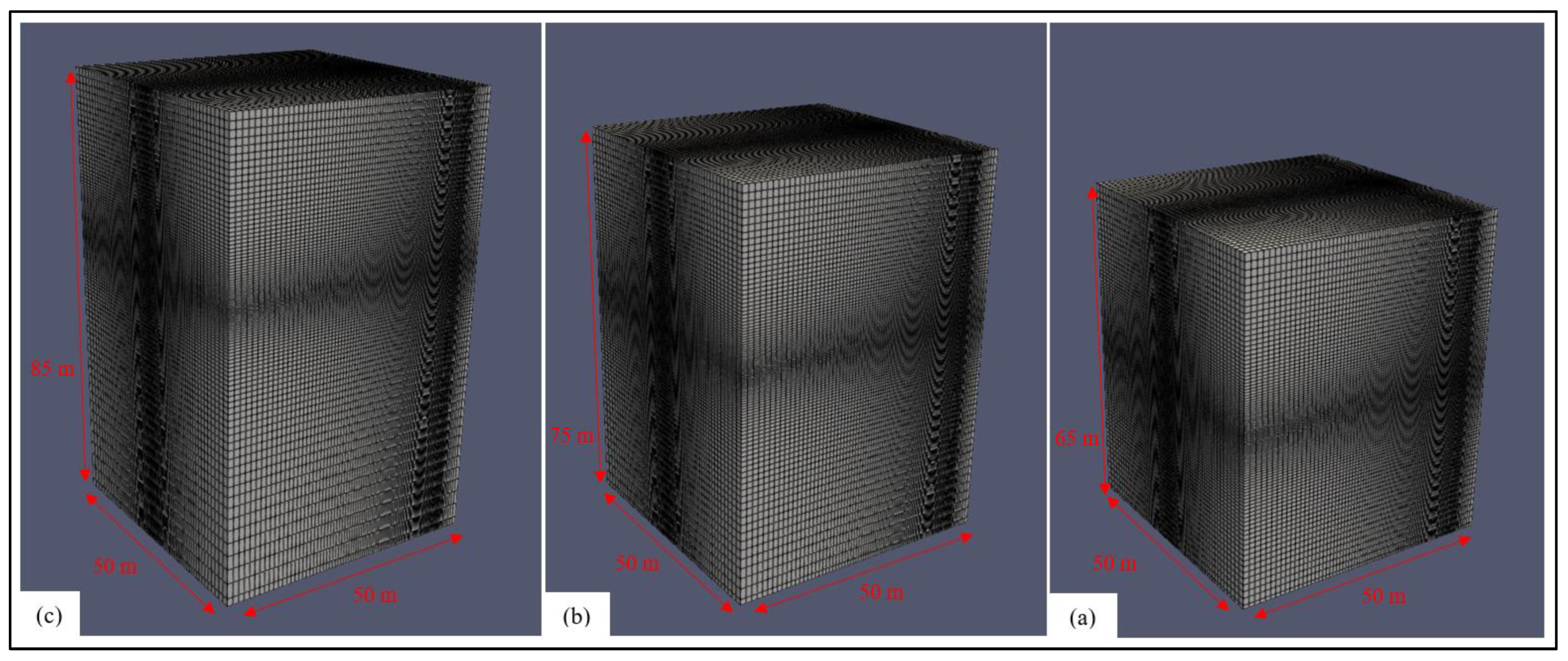
Figure 2.
Computational size and mesh: (a) 65 m (z-axis), 50 m (x-axis), and 50 (y-axis); (b) 75 m (z-axis), 50 m (x-axis), and 50 (y-axis); and (c) 85 m (z-axis), 50 m (x-axis), and 50 (y-axis).
Figure 2.
Computational size and mesh: (a) 65 m (z-axis), 50 m (x-axis), and 50 (y-axis); (b) 75 m (z-axis), 50 m (x-axis), and 50 (y-axis); and (c) 85 m (z-axis), 50 m (x-axis), and 50 (y-axis).
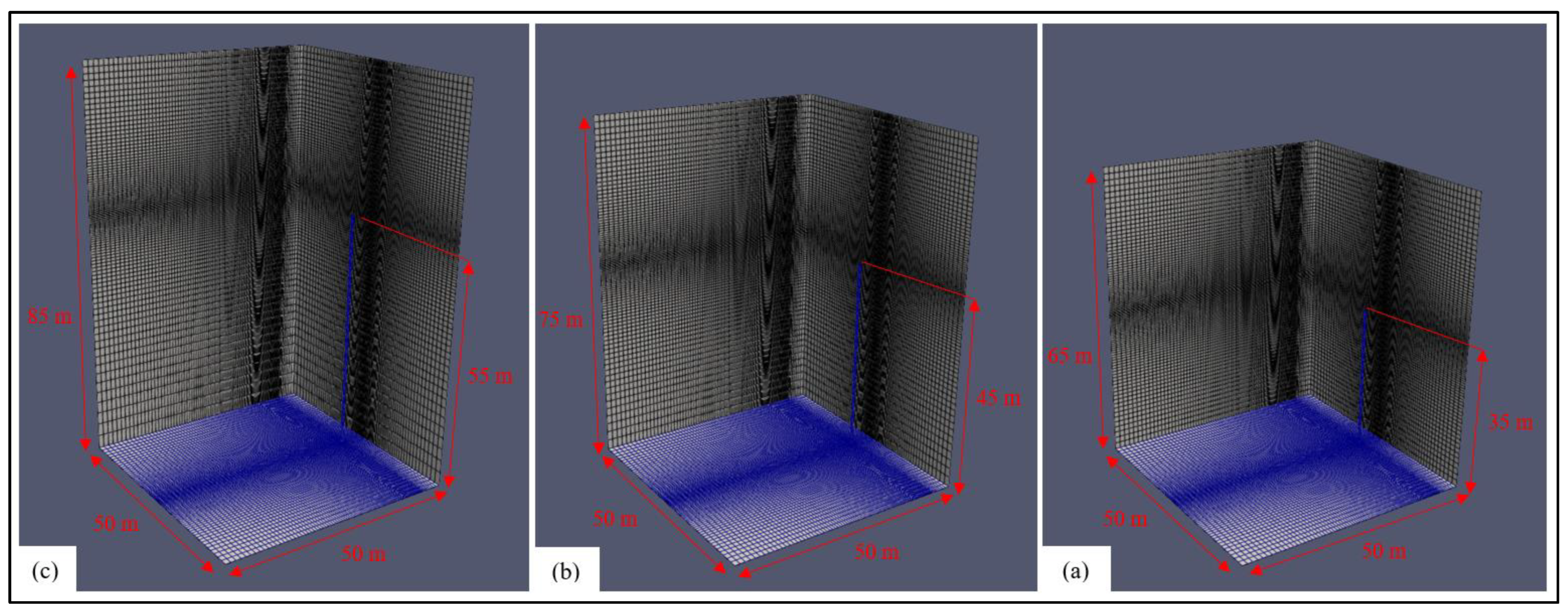
Figure 3.
Flare model and ground mesh: (a) 35 m stack height, (b) 45 m stack height, and (c) 55 m stack height.
Figure 3.
Flare model and ground mesh: (a) 35 m stack height, (b) 45 m stack height, and (c) 55 m stack height.
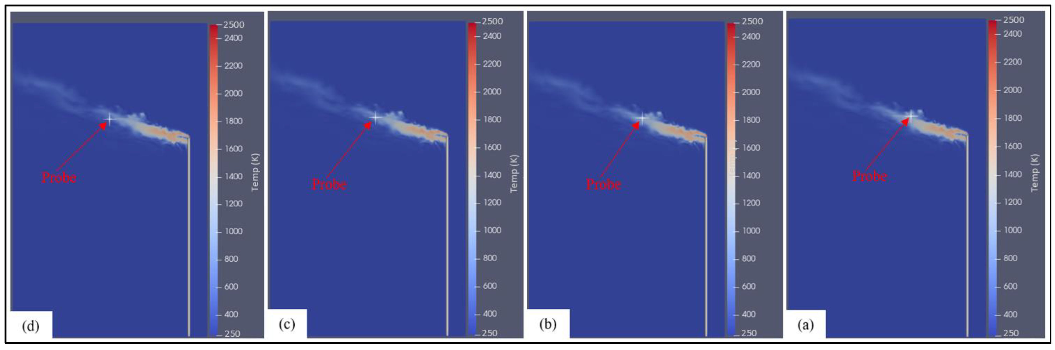
Figure 4.
Data sampling locations for the mesh independence study at a 9 t/h firing rate using a stack height of 55 m: (a) 14 m (x-axis), 0 m (y-axis), and 60 m (z-axis); (b) 16 m (x-axis), 0 m (y-axis), and 60 m (z-axis); (c) 18 m (x-axis), 0 m (y-axis), and 60 m (z-axis); and (d) 20 m (x-axis), 0 m (y-axis), and 60 m (z-axis).
Figure 5.
Data sampling locations for the mesh independence study at a 9 t/h firing rate using a stack height of 45 m: (a) 14 m (x-axis), 0 m (y-axis), and 50 m (z-axis); (b) 16 m (x-axis), 0 m (y-axis), and 50 m (z-axis); (c) 18 m (x-axis), 0 m (y-axis), and 50 m (z-axis); and (d) 20 m (x-axis), 0 m (y-axis), and 51 m (z-axis).
Figure 6.
Data sampling locations for the mesh independence study at a 9 t/h firing rate using a stack height of 35 m: (a) 12 m (x-axis), 0 m (y-axis), and 40 m (z-axis); (b) 14 m (x-axis), 0 m (y-axis), and 40 m (z-axis); (c) 16 m (x-axis), 0 m (y-axis), and 40 m (z-axis); and (d) 18 m (x-axis), 0 m (y-axis), and 40 m (z-axis).
Figure 7.
Mesh independence study of the 35 m tall stack case at a 9 t/h firing rate and 8 m/s crosswind.
Figure 7.
Mesh independence study of the 35 m tall stack case at a 9 t/h firing rate and 8 m/s crosswind.
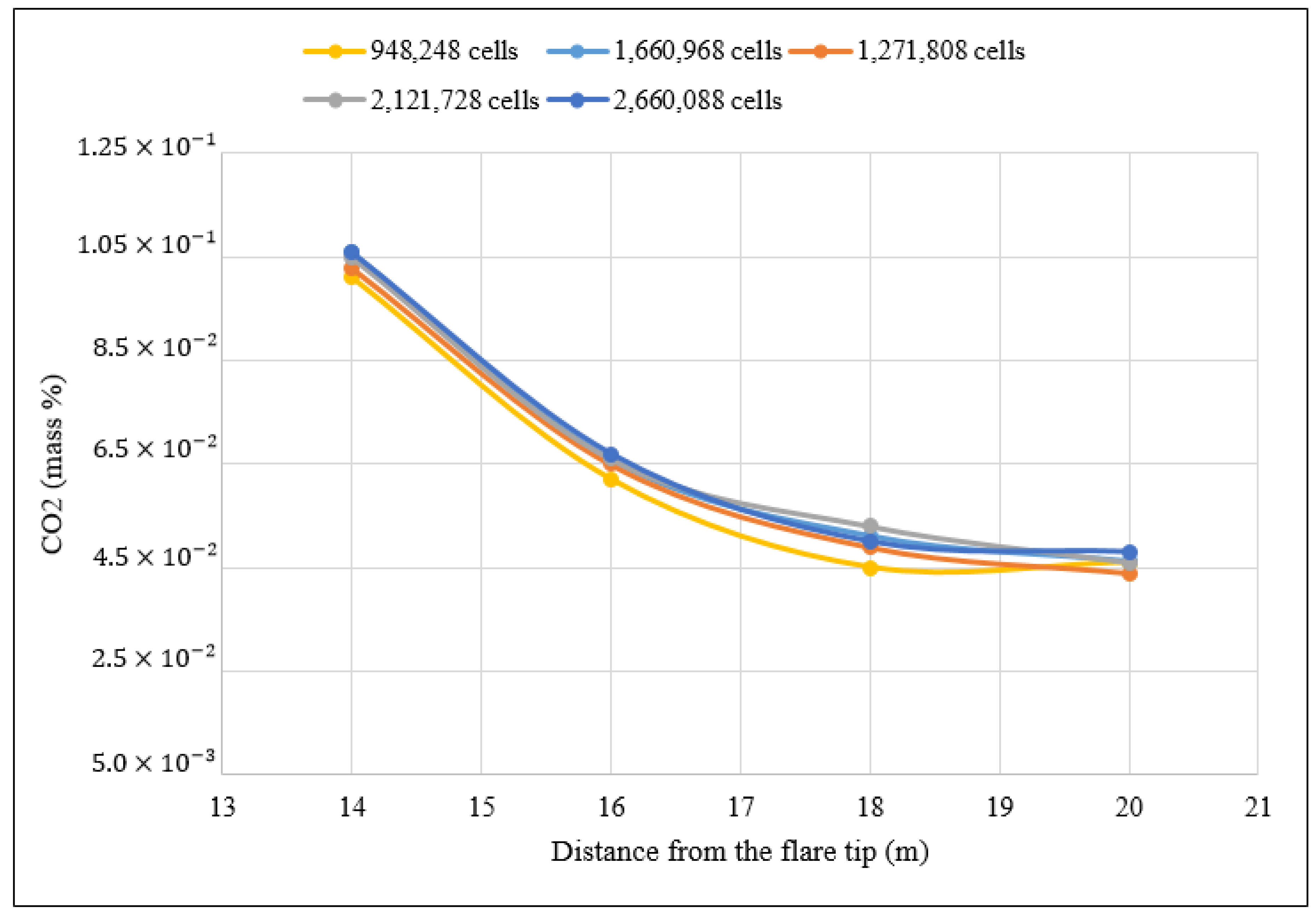
Figure 8.
Mesh independence study of the 45 m tall stack case at a 9 t/h firing rate and 8 m/s crosswind.
Figure 8.
Mesh independence study of the 45 m tall stack case at a 9 t/h firing rate and 8 m/s crosswind.
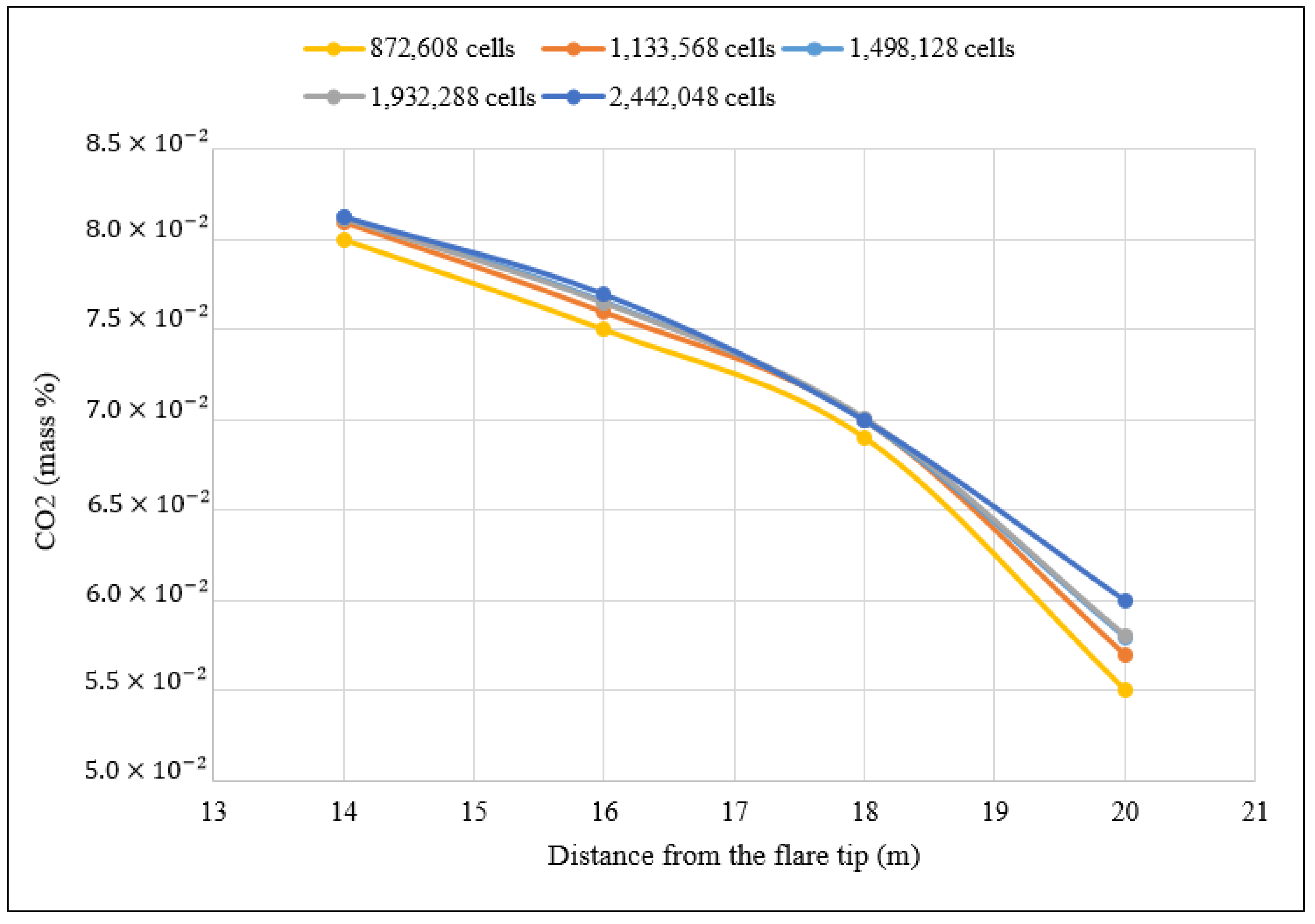
Figure 9.
Mesh independence study of the 55 m tall stack case at a 9 t/h firing rate and 8 m/s crosswind.
Figure 9.
Mesh independence study of the 55 m tall stack case at a 9 t/h firing rate and 8 m/s crosswind.
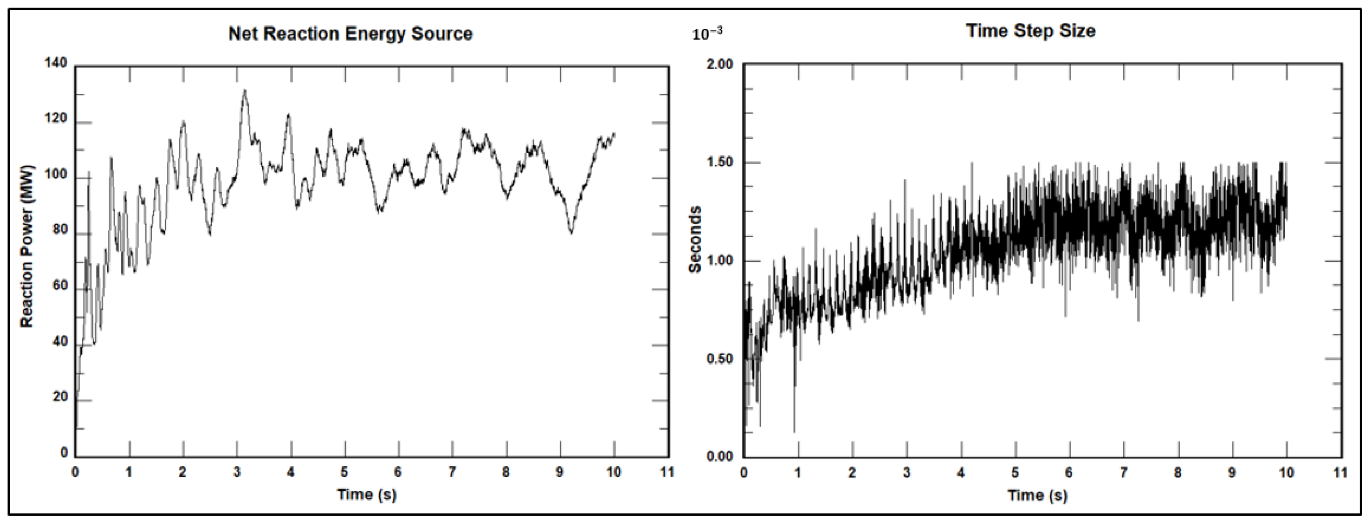
Figure 10.
Net reaction energy source and simulation time step size for 2.5 kg/s gas firing rate cases.
Figure 10.
Net reaction energy source and simulation time step size for 2.5 kg/s gas firing rate cases.
Figure 11.
Net reaction energy source and simulation time step size for 12.5 kg/s gas firing rate cases.
Figure 11.
Net reaction energy source and simulation time step size for 12.5 kg/s gas firing rate cases.
Figure 12.
Low gas firing rate (9 t/h) flare operation with three different crosswind speeds: (a) 4 m/s, (b) 8 m/s, and (c) 14 m/s.
Figure 12.
Low gas firing rate (9 t/h) flare operation with three different crosswind speeds: (a) 4 m/s, (b) 8 m/s, and (c) 14 m/s.
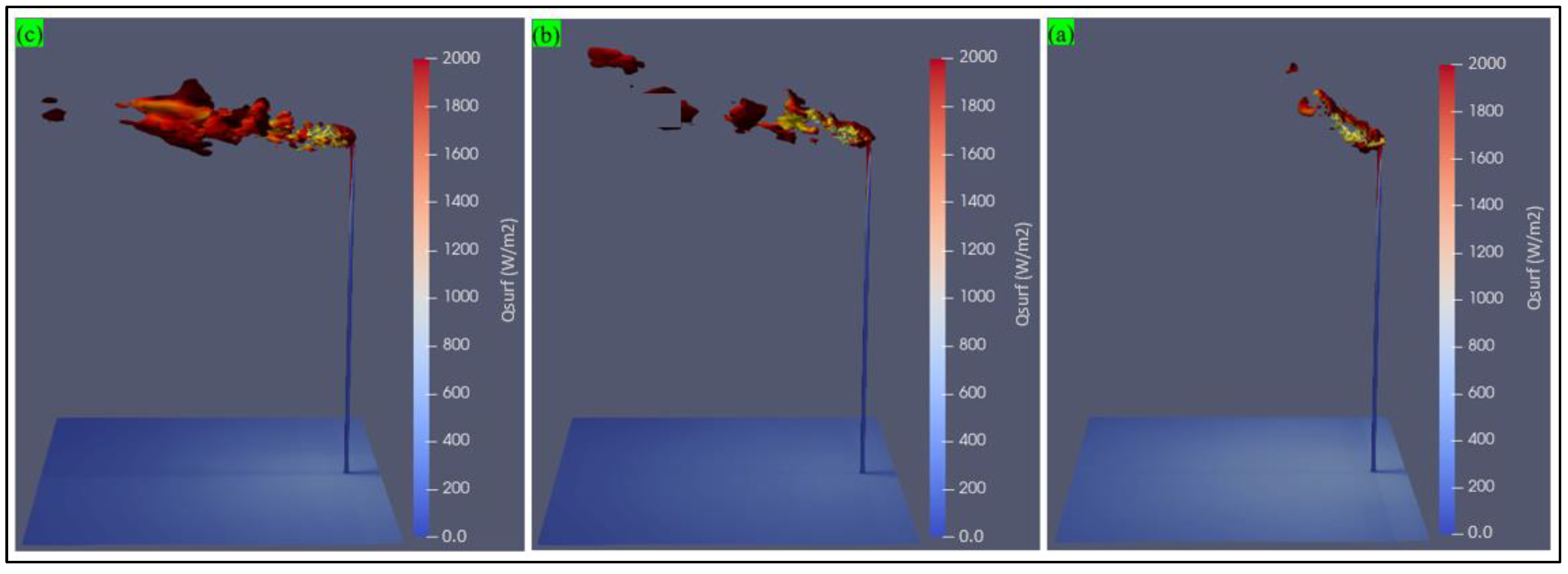
Figure 13.
High gas firing rate (45 t/h) flare operation with three different crosswind speeds: (a) 4 m/s, (b) 8 m/s, and (c) 14 m/s.
Figure 13.
High gas firing rate (45 t/h) flare operation with three different crosswind speeds: (a) 4 m/s, (b) 8 m/s, and (c) 14 m/s.
Figure 14.
Flame temperature at a normal gas firing rate (9 t/h) with different crosswind speeds: (a) 4 m/s, (b) 8 m/s, and (c) 14 m/s.
Figure 14.
Flame temperature at a normal gas firing rate (9 t/h) with different crosswind speeds: (a) 4 m/s, (b) 8 m/s, and (c) 14 m/s.
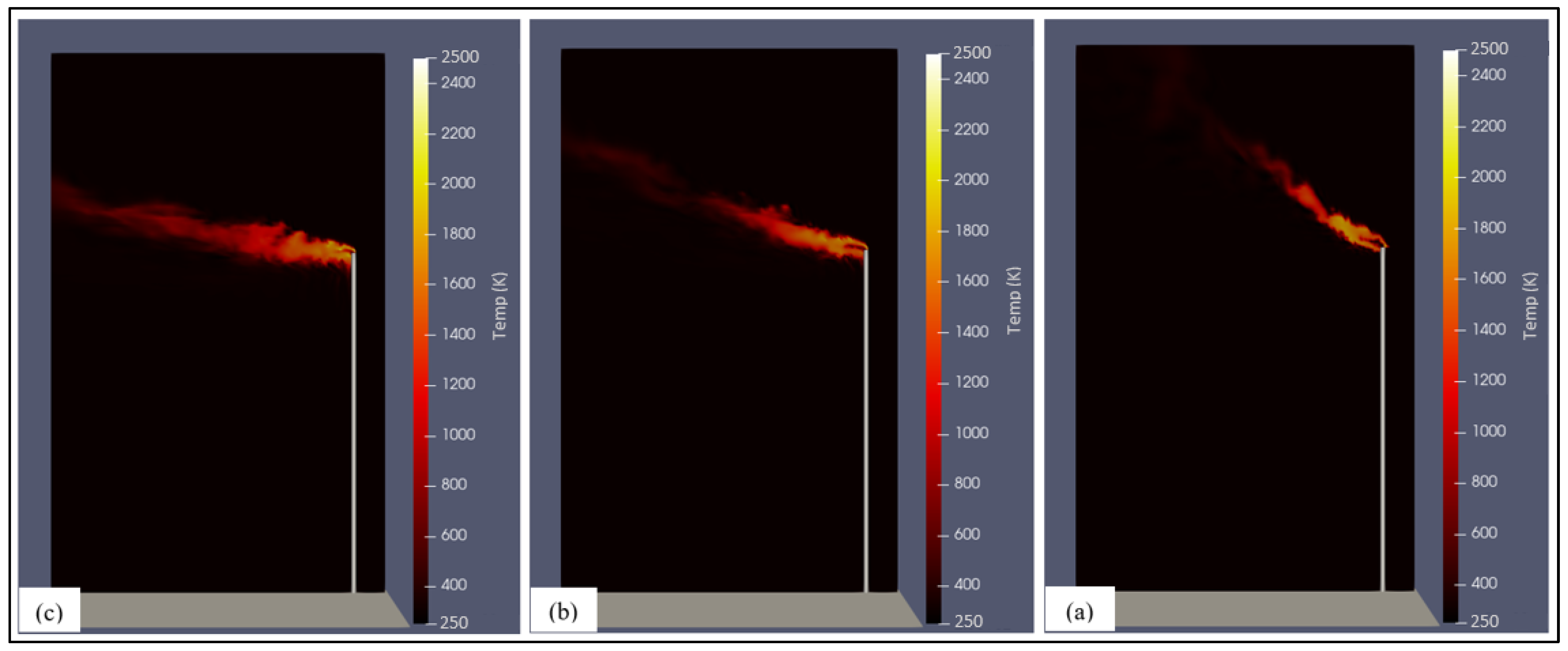
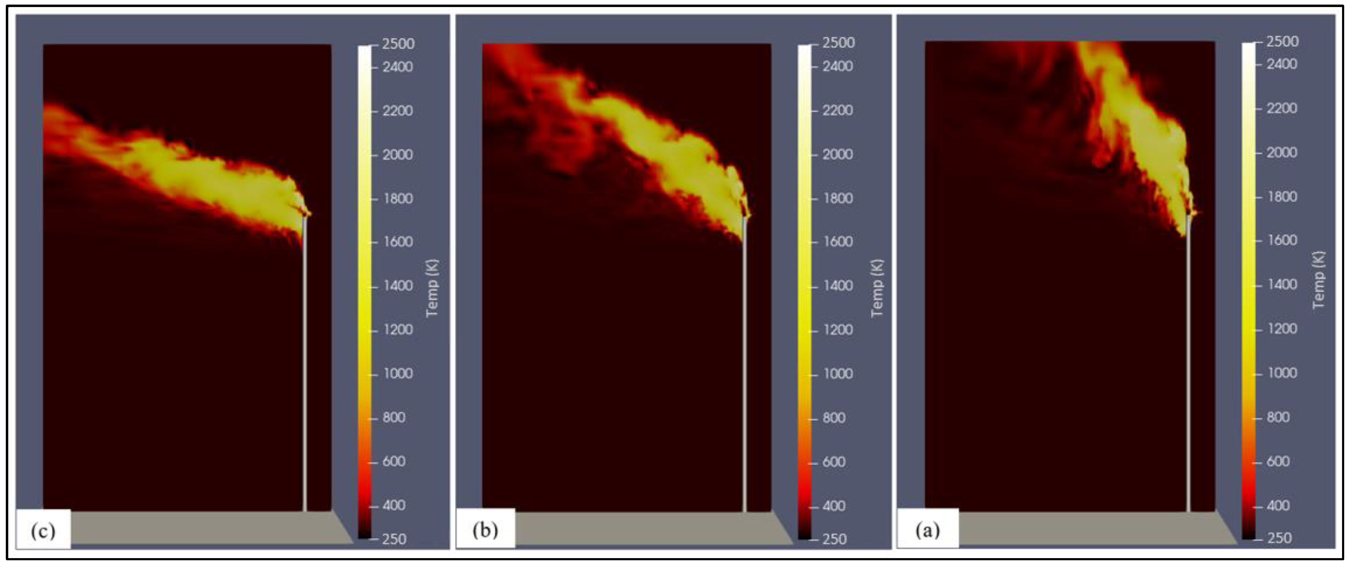
Figure 15.
Flame temperature at a high gas firing rate (45 t/h) with different crosswind speeds: (a) 4 m/s, (b) 8 m/s, and (c) 14 m/s.
Figure 15.
Flame temperature at a high gas firing rate (45 t/h) with different crosswind speeds: (a) 4 m/s, (b) 8 m/s, and (c) 14 m/s.
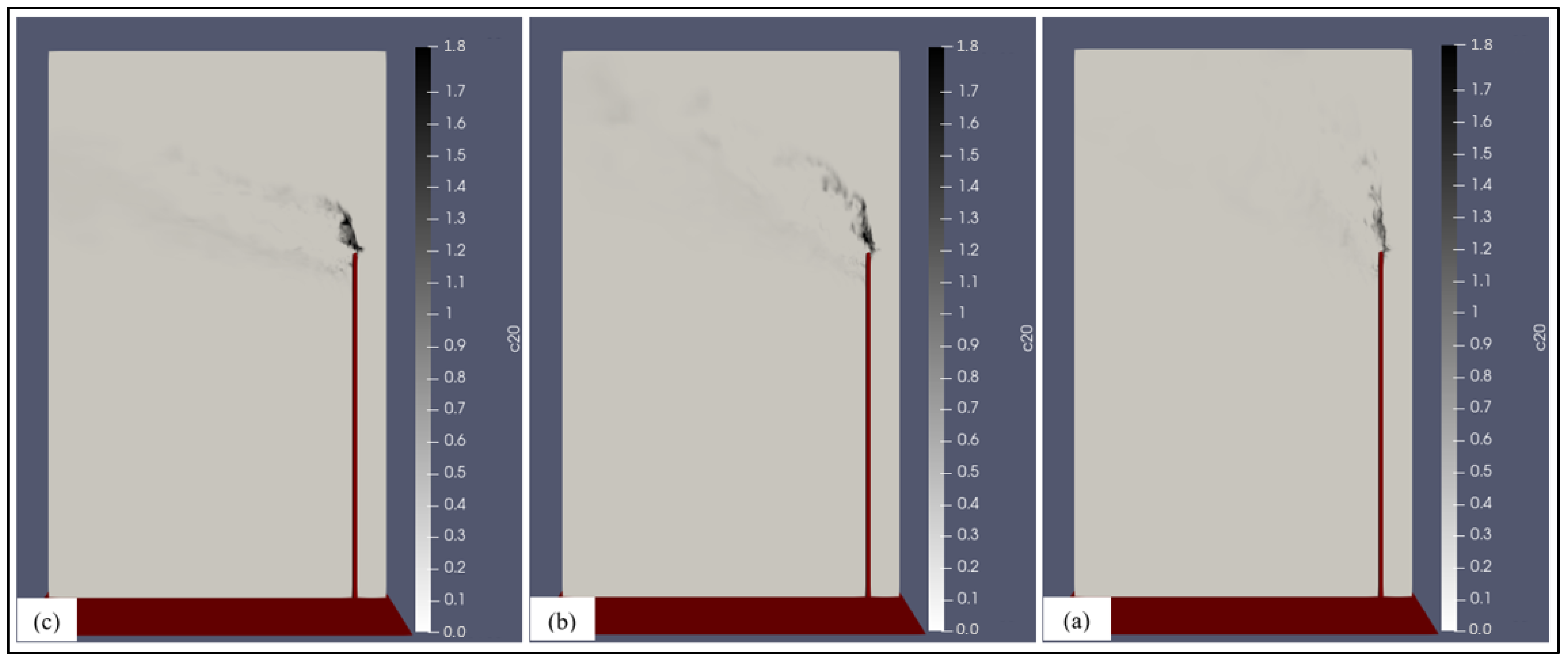
Figure 16.
Soot formation at a normal gas firing rate (9 t/h) with different crosswind speeds: (a) 4 m/s, (b) 8 m/s, and (c) 14 m/s.
Figure 16.
Soot formation at a normal gas firing rate (9 t/h) with different crosswind speeds: (a) 4 m/s, (b) 8 m/s, and (c) 14 m/s.
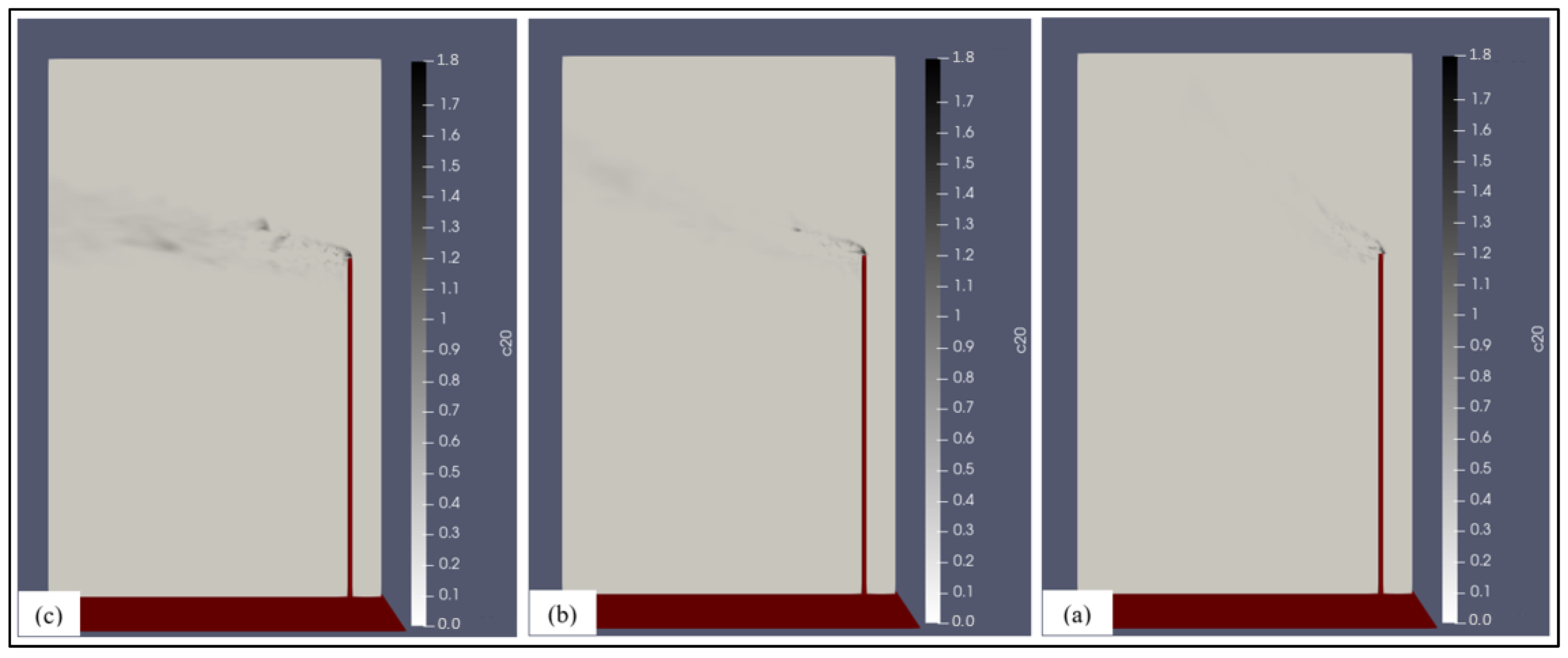
Figure 17.
Soot formation at a high gas firing rate (45 t/h) with different crosswind speeds: (a) 4 m/s, (b) 8 m/s, and (c) 14 m/s.
Figure 17.
Soot formation at a high gas firing rate (45 t/h) with different crosswind speeds: (a) 4 m/s, (b) 8 m/s, and (c) 14 m/s.
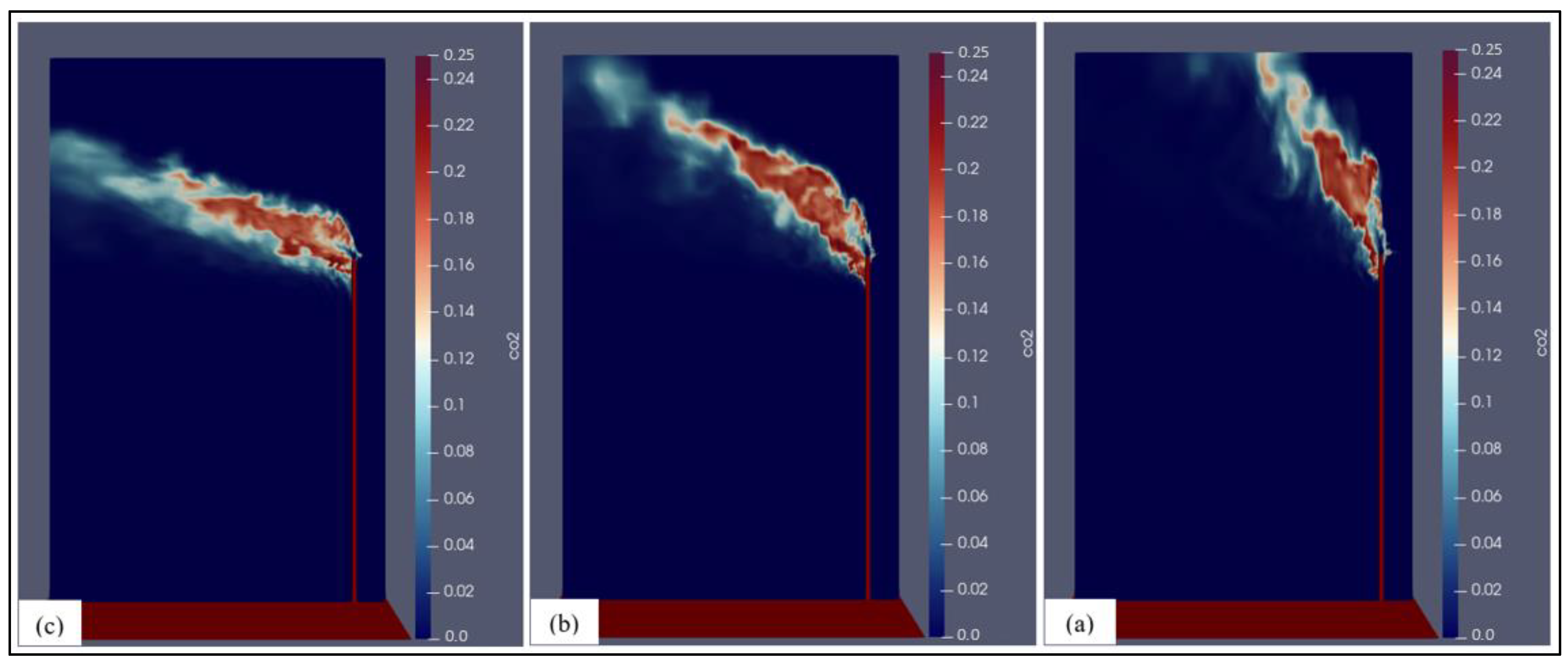
Figure 18.
Carbon dioxide emissions at a normal gas firing rate (9 t/h) with different crosswind speeds: (a) 4 m/s, (b) 8 m/s, and (c) 14 m/s.
Figure 18.
Carbon dioxide emissions at a normal gas firing rate (9 t/h) with different crosswind speeds: (a) 4 m/s, (b) 8 m/s, and (c) 14 m/s.
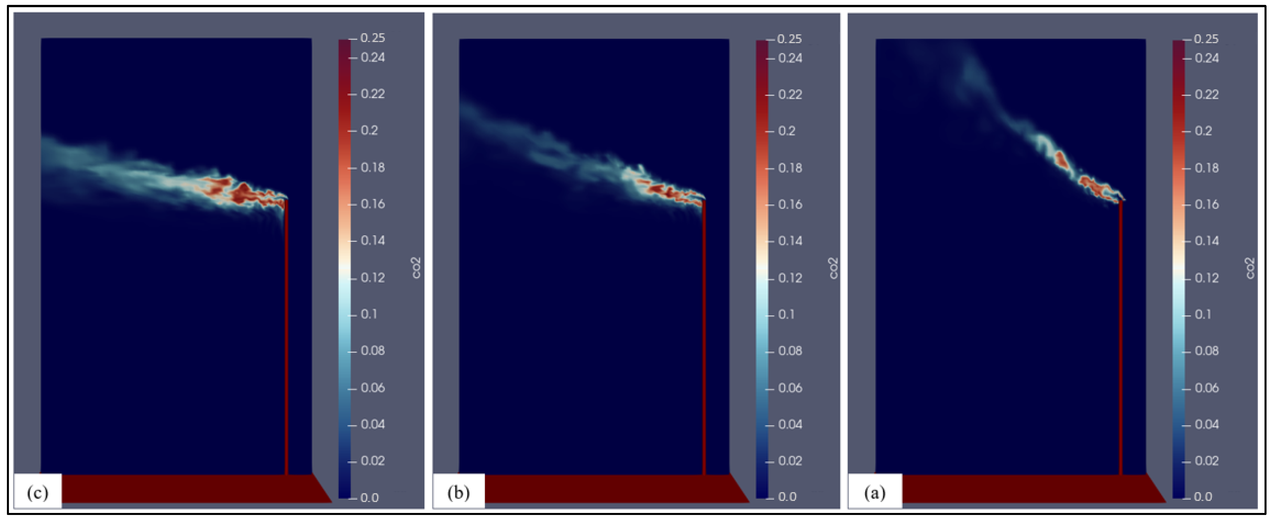
Figure 19.
Carbon dioxide emissions at a high gas firing rate (45 t/h) with different crosswind speeds: (a) 4 m/s, (b) 8 m/s, and (c) 14 m/s.
Figure 19.
Carbon dioxide emissions at a high gas firing rate (45 t/h) with different crosswind speeds: (a) 4 m/s, (b) 8 m/s, and (c) 14 m/s.
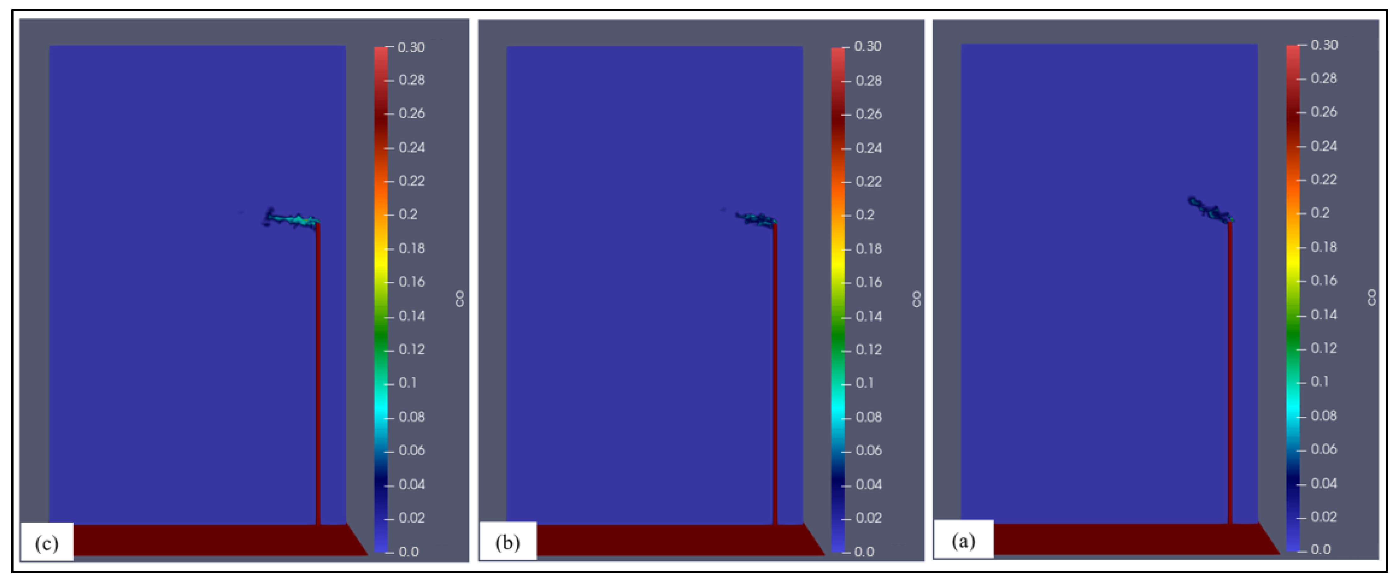
Figure 20.
Carbon monoxide emissions at a normal gas firing rate (9 t/h) with different crosswind speeds: (a) 4 m/s, (b) 8 m/s, and (c) 14 m/s.
Figure 20.
Carbon monoxide emissions at a normal gas firing rate (9 t/h) with different crosswind speeds: (a) 4 m/s, (b) 8 m/s, and (c) 14 m/s.
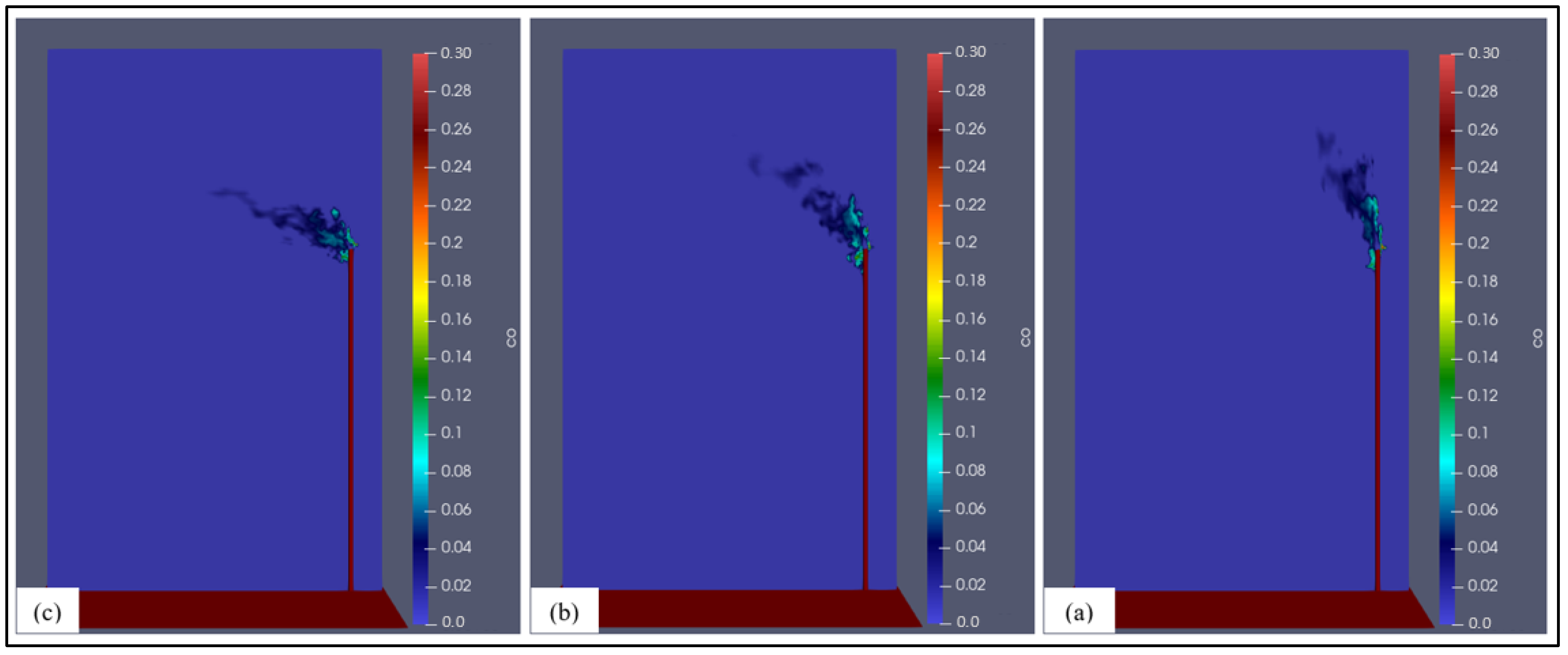
Figure 21.
Carbon monoxide emissions at a high gas firing rate (45 t/h) with different crosswind speeds: (a) 4 m/s, (b) 8 m/s, and (c) 14 m/s.
Figure 21.
Carbon monoxide emissions at a high gas firing rate (45 t/h) with different crosswind speeds: (a) 4 m/s, (b) 8 m/s, and (c) 14 m/s.
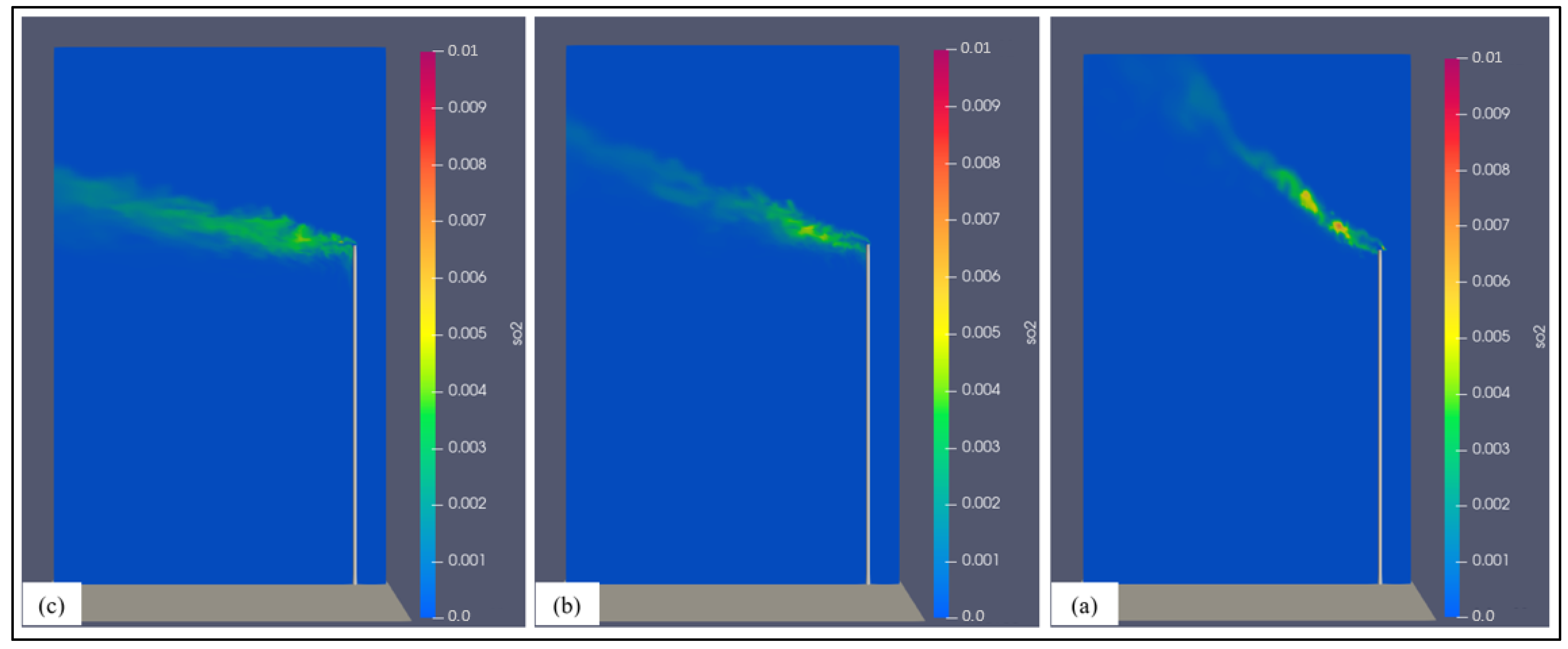
Figure 22.
Sulphur dioxide emissions at a normal gas firing rate (9 t/h) with different crosswind speeds: (a) 4 m/s, (b) 8 m/s, and (c) 14 m/s.
Figure 22.
Sulphur dioxide emissions at a normal gas firing rate (9 t/h) with different crosswind speeds: (a) 4 m/s, (b) 8 m/s, and (c) 14 m/s.
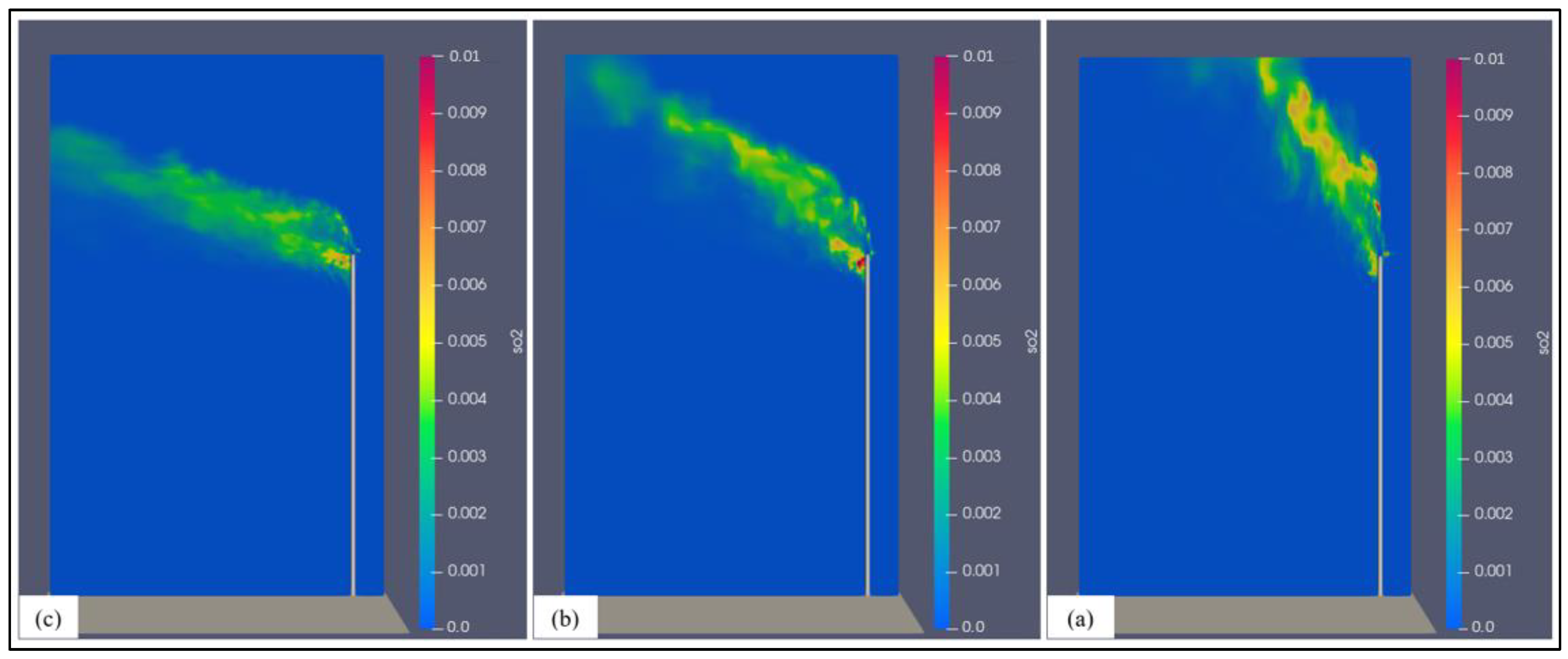
Figure 23.
Sulphur dioxide emissions at a high gas firing rate (45 t/h) with different crosswind speeds: (a) 4 m/s, (b) 8 m/s and (c) 14 m/s.
Figure 23.
Sulphur dioxide emissions at a high gas firing rate (45 t/h) with different crosswind speeds: (a) 4 m/s, (b) 8 m/s and (c) 14 m/s.
Figure 24.
Nitric oxide emissions at a normal gas firing rate (9 t/h) with different crosswind speeds: (a) 4 m/s, (b) 8 m/s, and (c) 14 m/s.
Figure 24.
Nitric oxide emissions at a normal gas firing rate (9 t/h) with different crosswind speeds: (a) 4 m/s, (b) 8 m/s, and (c) 14 m/s.
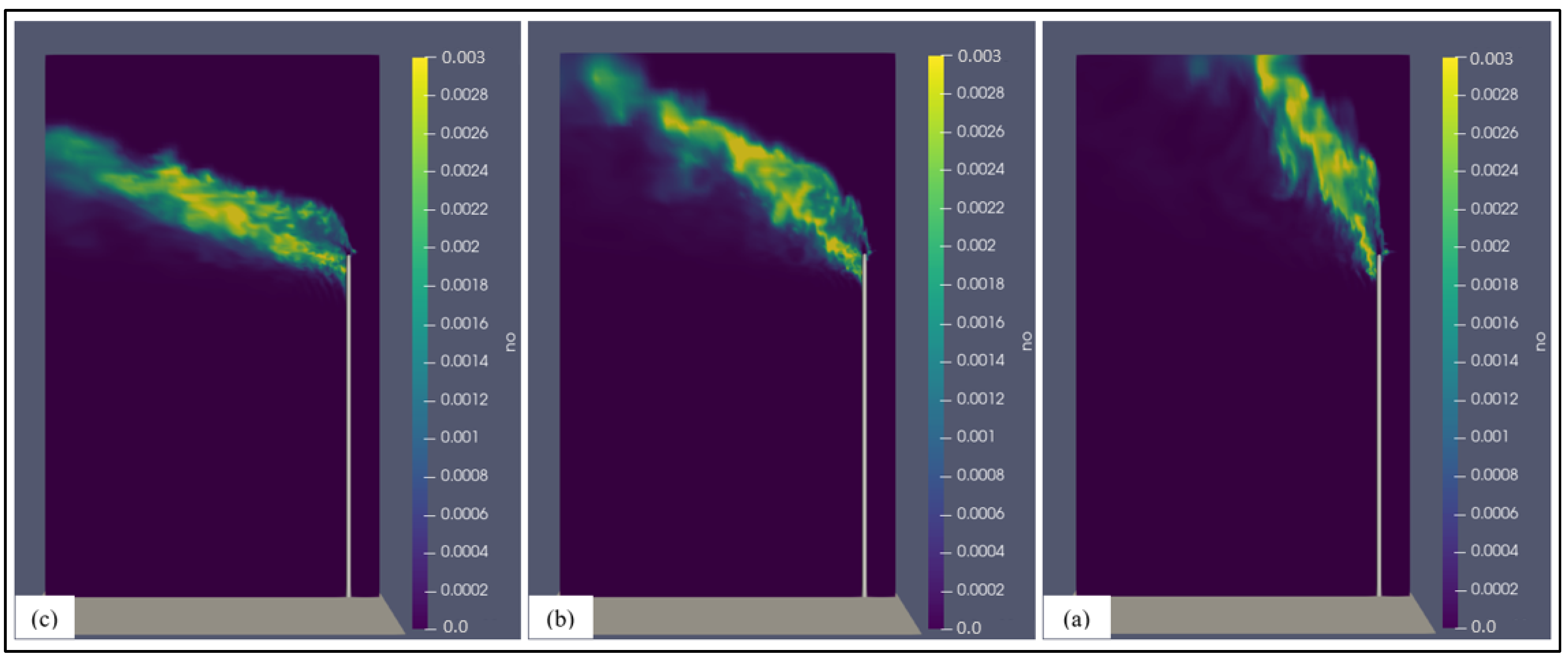
Figure 25.
Nitric oxide emissions at a high gas firing rate (45 t/h) with different crosswind speeds: (a) 4 m/s, (b) 8 m/s, and (c) 14 m/s.
Figure 25.
Nitric oxide emissions at a high gas firing rate (45 t/h) with different crosswind speeds: (a) 4 m/s, (b) 8 m/s, and (c) 14 m/s.
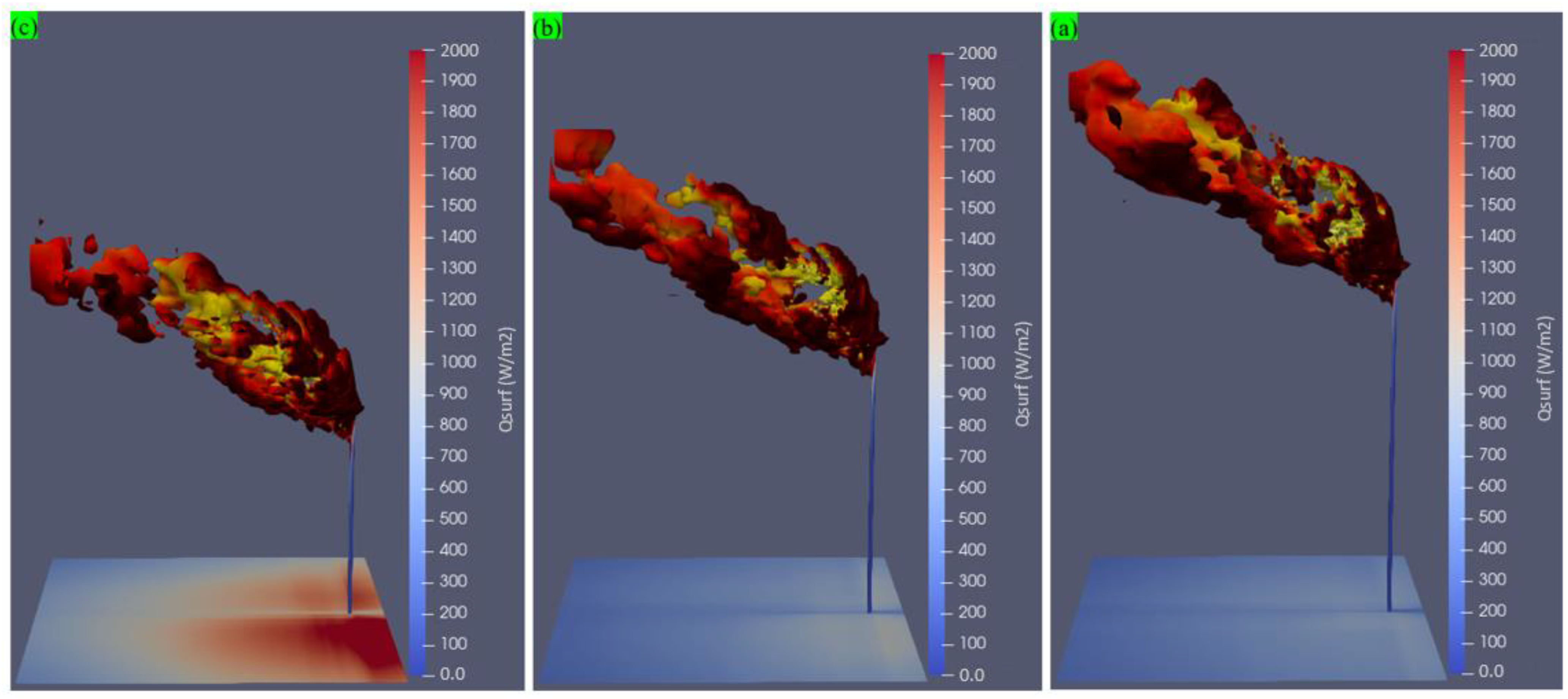
Figure 26.
Low gas firing rate (9 t/h) flare operation using three different stack heights: (a) 55 m, (b) 45 m, and (c) 35 m.
Figure 26.
Low gas firing rate (9 t/h) flare operation using three different stack heights: (a) 55 m, (b) 45 m, and (c) 35 m.
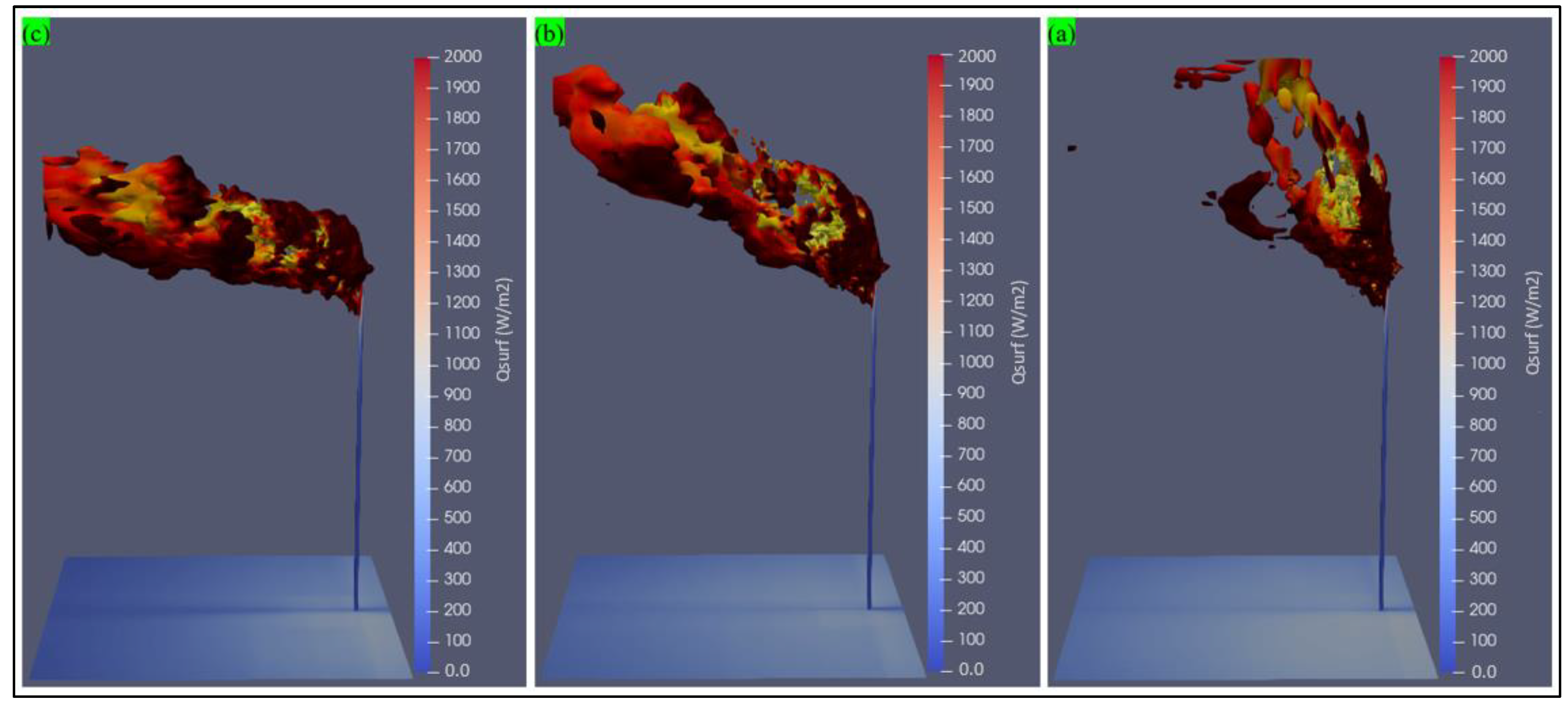
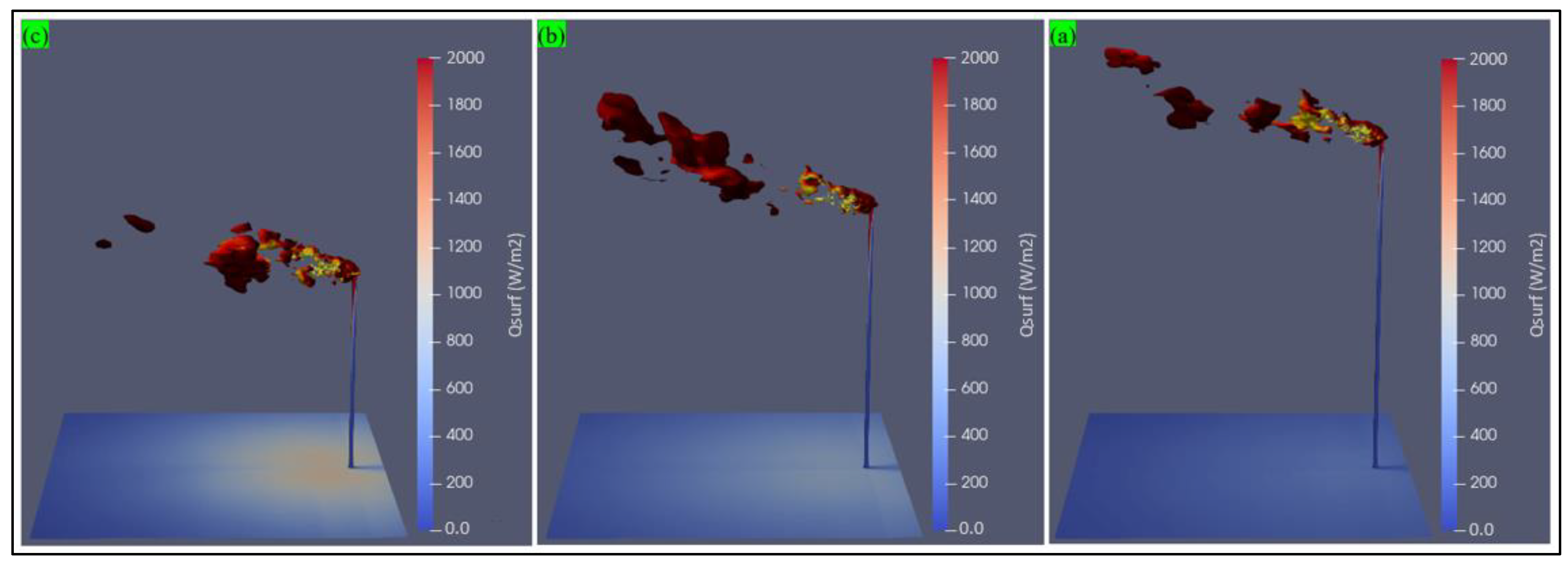
Figure 27.
High gas firing rate (45 t/h) flare operation using three different stack heights: (a) 55 m, (b) 45 m, and (c) 35 m.
Figure 27.
High gas firing rate (45 t/h) flare operation using three different stack heights: (a) 55 m, (b) 45 m, and (c) 35 m.
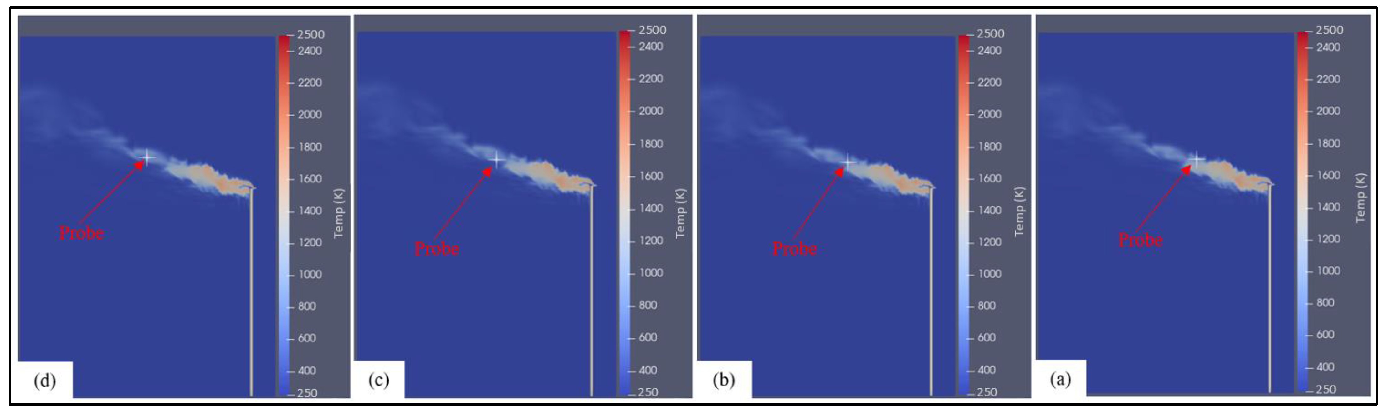
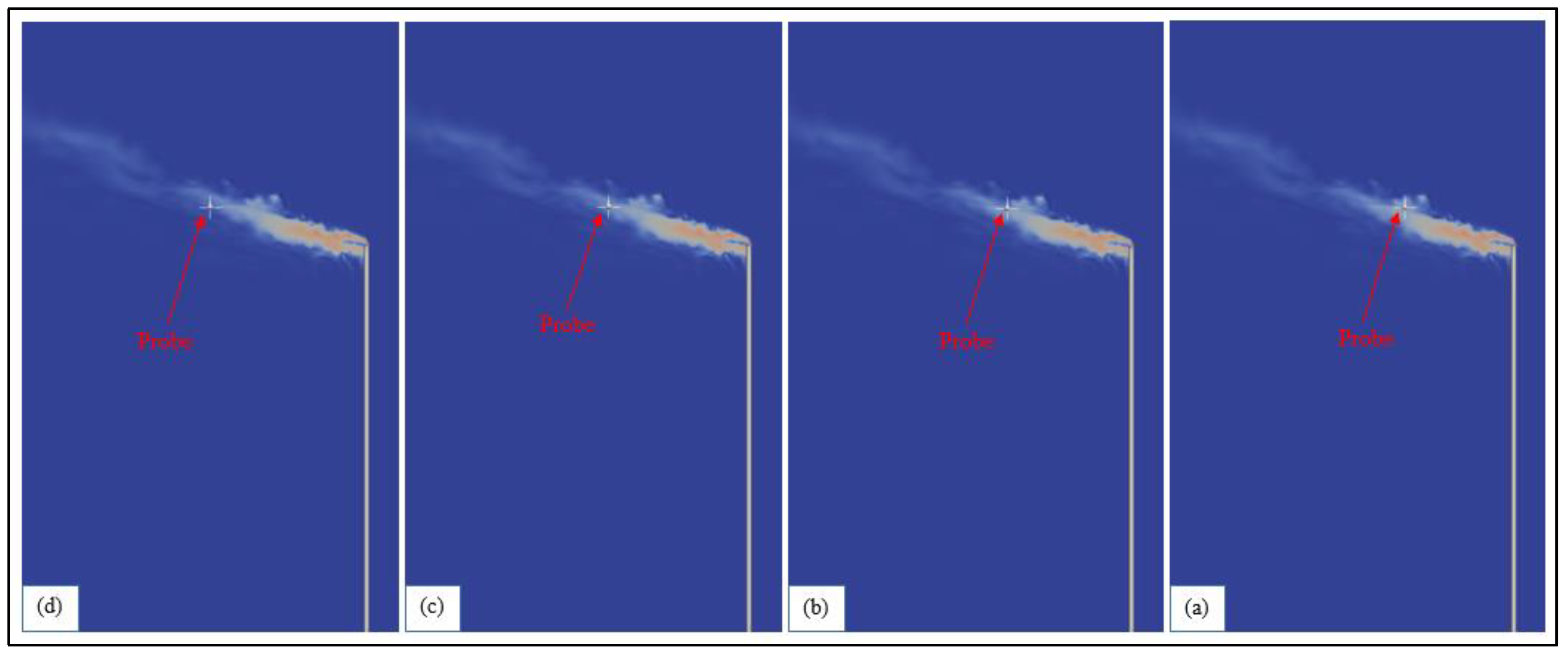
Figure 28.
Probe locations at a normal gas firing rate (9 t/h) of the flare using a stack height of 55 m: (a) 14 m (x-axis), 0 m (y-axis), 60 m (z-axis); (b) 16 m (x-axis), 0 m (y-axis), 60 m (z-axis); (c) 18 m (x-axis), 0 m (y-axis), 60 m (z-axis); and (d) 20 m (x-axis), 0 m (y-axis), 60 m (z-axis).
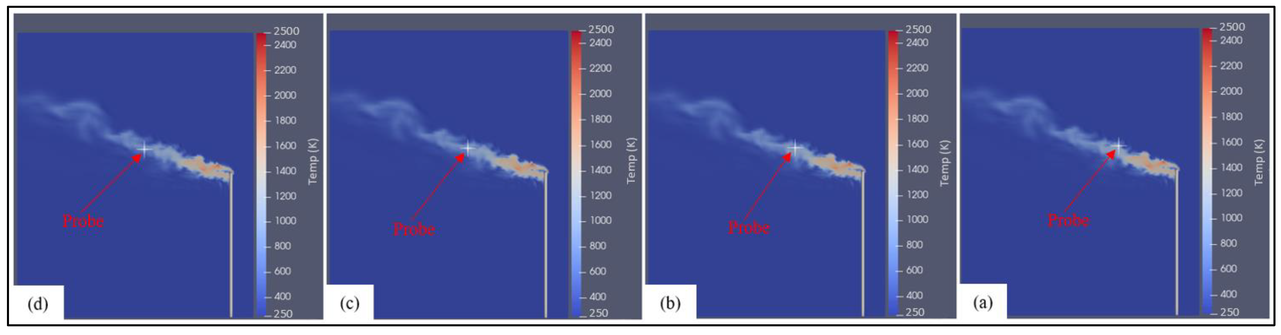
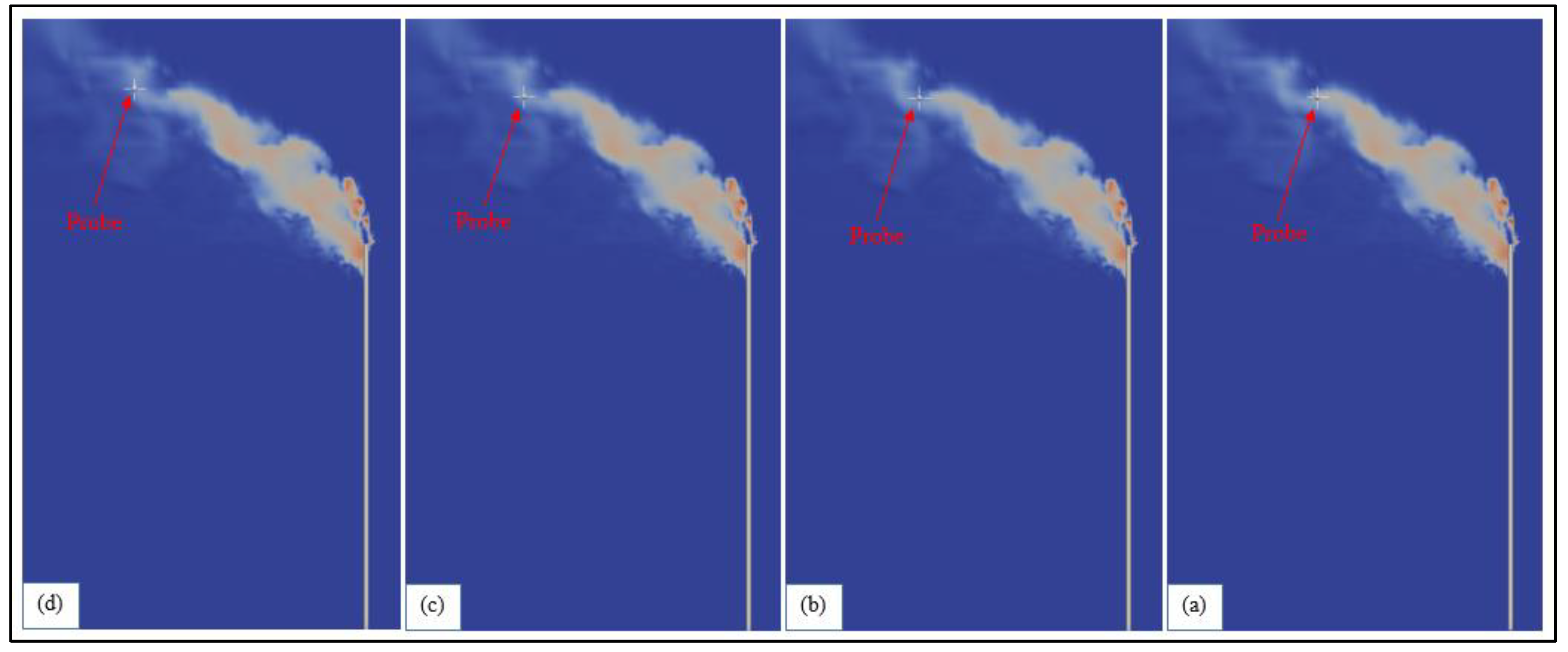
Figure 29.
Probe locations at a high gas firing rate (45 t/h) of the flare using a stack height of 55 m: (a) 25 m (x-axis), 0 m (y-axis), 74 m (z-axis); (b) 27 m (x-axis), 0 m (y-axis), 74 m (z-axis); (c) 29 m (x-axis), 0 m (y-axis), 74 m (z-axis); and (d) 30 m (x-axis), 0 m (y-axis), 75 m (z-axis)..
Table 1.
Case study flare gas composition.
Table 1.
Case study flare gas composition.
| Basis = 100 kg Mole |
|---|
| Components | Mole (%) | Mole (kg Mole) | MWt (kg/kg Mole) | Mass (kg) | Mass (%) |
|---|
| CH4 | 16.44 | 16.44 | 16 | 263.0 | 0.074 |
| C2H6 | 8.80 | 8.80 | 30 | 264.0 | 0.074 |
| C3H8 | 12.5 | 12.5 | 44 | 550.0 | 0.155 |
| C4H10 | 20.35 | 20.35 | 58 | 1180.3 | 0.333 |
| C5H12 | 14.37 | 14.37 | 72 | 1034.6 | 0.292 |
| H2S | 2.96 | 2.96 | 34 | 100.6 | 0.028 |
| H2 | 20.58 | 20.58 | 2 | 41.2 | 0.012 |
| N2 | 4.00 | 4.00 | 28 | 112.0 | 0.032 |
| Total | 100 | 100.0 | | 3545.8 | 1.00 |
Table 2.
Main combustion products at a normal gas firing rate (9 t/h).
Table 2.
Main combustion products at a normal gas firing rate (9 t/h).
| Probe Location | CO (Mass%) | CO2 (Mass%) | Soot (Mass%) | SO2 (Mass%) | NO (Mass%) |
|---|
| x-Axis (m) | y-Axis (m) | z-Axis (m) | Radius (m) |
|---|
| 14 | 0 | 60 | 0.3 | 6.31 × 10⁻⁹ | 1.06 × 10⁻¹ | 1.90 × 10⁻⁴ | 2.49 × 10⁻³ | 2.33 × 10⁻³ |
| 16 | 0 | 60 | 0.3 | 3.26 × 10⁻⁷ | 6.58 × 10⁻² | 9.90 × 10⁻⁵ | 1.60 × 10⁻³ | 1.47 × 10⁻³ |
| 18 | 0 | 60 | 0.3 | 4.52 × 10⁻⁹ | 5.10 × 10⁻² | 1.42 × 10⁻⁴ | 1.22 × 10⁻³ | 1.14 × 10⁻³ |
| 20 | 0 | 60 | 0.3 | 1.28 × 10⁻⁶ | 4.61 × 10⁻² | 2.51 × 10⁻⁴ | 1.11 × 10⁻³ | 1.02 × 10⁻³ |
Table 3.
Main fuel compounds in the plume at a normal gas firing rate (9 t/h).
Table 3.
Main fuel compounds in the plume at a normal gas firing rate (9 t/h).
| Probe Location | CH4 (Mass%) | C2H6 (Mass%) | C3H8 (Mass%) | C4H10 (Mass%) | C5H12 (Mass%) |
|---|
| x-Axis (m) | y-Axis (m) | z-Axis (m) | Radius (m) |
|---|
| 14 | 0 | 60 | 0.3 | 8.43 × 10⁻⁹ | 7.42 × 10⁻⁹ | 7.51 × 10⁻⁹ | 7.63 × 10⁻⁹ | 7.59 × 10⁻⁹ |
| 16 | 0 | 60 | 0.3 | 7.83 × 10⁻⁹ | 6.04 × 10⁻⁹ | 6.14 × 10⁻⁹ | 6.32 × 10⁻⁹ | 6.31 × 10⁻⁹ |
| 18 | 0 | 60 | 0.3 | 7.80 × 10⁻⁹ | 5.30 × 10⁻⁹ | 5.41 × 10⁻⁹ | 5.62 × 10⁻⁹ | 5.62 × 10⁻⁹ |
| 20 | 0 | 60 | 0.3 | 6.96 × 10⁻⁹ | 4.72 × 10⁻⁹ | 4.83 × 10⁻⁹ | 5.01 × 10⁻⁹ | 5.00 × 10⁻⁹ |
Table 4.
Main combustion products at a high gas firing rate (45 t/h).
Table 4.
Main combustion products at a high gas firing rate (45 t/h).
| Probe Location | CO (Mass%) | CO2 (Mass%) | Soot (Mass%) | SO2 (Mass%) | NO (Mass%) |
|---|
| x-Axis (m) | y-Axis (m) | z-Axis (m) | Radius (m) |
|---|
| 25 | 0 | 74 | 0.3 | 1.45 × 10⁻⁵ | 1.24 × 10⁻¹ | 1.76 × 10⁻⁵ | 3.39 × 10⁻³ | 2.39 × 10⁻³ |
| 27 | 0 | 74 | 0.3 | 1.16 × 10⁻⁸ | 1.38 × 10⁻¹ | 7.06 × 10⁻⁵ | 3.91 × 10⁻³ | 2.76 × 10⁻³ |
| 29 | 0 | 74 | 0.3 | 2.66 × 10⁻⁸ | 1.27 × 10⁻¹ | 3.82 × 10⁻⁵ | 3.82 × 10⁻³ | 2.67 × 10⁻³ |
| 30 | 0 | 75 | 0.3 | 2.83 × 10⁻⁷ | 7.78 × 10⁻² | 1.05 × 10⁻⁴ | 2.27 × 10⁻³ | 1.67 × 10⁻³ |
Table 5.
Main fuel compounds in the plume at a high gas firing rate (45 t/h).
Table 5.
Main fuel compounds in the plume at a high gas firing rate (45 t/h).
| Probe Location | CH4 (Mass%) | C2H6 (Mass%) | C3H8 (Mass%) | C4H10 (Mass%) | C5H12 (Mass%) |
|---|
| x-Axis (m) | y-Axis (m) | z-Axis (m) | Radius (m) |
|---|
| 25 | 0 | 74 | 0.3 | 7.59 × 10⁻⁸ | 1.04 × 10⁻⁶ | 1.61 × 10⁻⁶ | 4.93 × 10⁻⁶ | 4.38 × 10⁻⁶ |
| 27 | 0 | 74 | 0.3 | 9.47 × 10⁻⁹ | 9.60 × 10⁻⁹ | 9.52 × 10⁻⁹ | 9.83 × 10⁻⁹ | 9.69 × 10⁻⁹ |
| 29 | 0 | 74 | 0.3 | 9.06 × 10⁻⁹ | 8.39 × 10⁻⁹ | 8.44 × 10⁻⁹ | 8.59 × 10⁻⁹ | 8.68 × 10⁻⁹ |
| 30 | 0 | 75 | 0.3 | 8.69 × 10⁻⁹ | 6.29 × 10⁻⁹ | 6.40 × 10⁻⁹ | 6.60 × 10⁻⁹ | 6.59 × 10⁻⁹ |
Table 6.
Main flare gas compounds in the fuel and the plume at a normal gas firing rate (9 t/h).
Table 6.
Main flare gas compounds in the fuel and the plume at a normal gas firing rate (9 t/h).
| Plume | | | | | |
|---|
| Probe Location | CH4 (Mass%) | C2H6 (Mass%) | C3H8 (Mass%) | C4H10 (Mass%) | C5H12 (Mass%) |
|---|
| x-Axis (m) | y-Axis (m) | z-Axis (m) | Radius (m) |
|---|
| 14 | 0 | 60 | 0.3 | 8.43 × 10⁻⁹ | 7.42 × 10⁻⁹ | 7.51 × 10⁻⁹ | 7.63 × 10⁻⁹ | 7.59 × 10⁻⁹ |
| 16 | 0 | 60 | 0.3 | 7.83 × 10⁻⁹ | 6.04 × 10⁻⁹ | 6.14 × 10⁻⁹ | 6.32 × 10⁻⁹ | 6.31 × 10⁻⁹ |
| 18 | 0 | 60 | 0.3 | 7.80 × 10⁻⁹ | 5.30 × 10⁻⁹ | 5.41 × 10⁻⁹ | 5.62 × 10⁻⁹ | 5.62 × 10⁻⁹ |
| 20 | 0 | 60 | 0.3 | 6.96 × 10⁻⁹ | 4.72 × 10⁻⁹ | 4.83 × 10⁻⁹ | 5.01 × 10⁻⁹ | 5.00 × 10⁻⁹ |
| Fuel | 7.40 × 10⁻² | 7.40 × 10⁻² | 1.55 × 10⁻¹ | 3.33 × 10⁻¹ | 2.92 × 10⁻¹ |
Table 7.
Main flare gas compounds in the fuel and the plume at a high gas firing rate (45 t/h).
Table 7.
Main flare gas compounds in the fuel and the plume at a high gas firing rate (45 t/h).
| Plume | | | | | |
|---|
| Probe Location | CH4 (Mass%) | C2H6 (Mass%) | C3H8 (Mass%) | C4H10 (Mass%) | C5H12 (Mass%) |
|---|
| x-Axis (m) | y-Axis (m) | z-Axis (m) | Radius (m) |
|---|
| 14 | 0 | 60 | 0.3 | 7.59 × 10⁻⁸ | 1.04 × 10⁻⁶ | 1.61 × 10⁻⁶ | 4.93 × 10⁻⁶ | 4.38 × 10⁻⁶ |
| 16 | 0 | 60 | 0.3 | 9.47 × 10⁻⁹ | 9.60 × 10⁻⁹ | 9.52 × 10⁻⁹ | 9.83 × 10⁻⁹ | 9.69 × 10⁻⁹ |
| 18 | 0 | 60 | 0.3 | 9.06 × 10⁻⁹ | 8.39 × 10⁻⁹ | 8.44 × 10⁻⁹ | 8.59 × 10⁻⁹ | 8.68 × 10⁻⁹ |
| 20 | 0 | 60 | 0.3 | 8.69 × 10⁻⁹ | 6.29 × 10⁻⁹ | 6.40 × 10⁻⁹ | 6.60 × 10⁻⁹ | 6.59 × 10⁻⁹ |
| Fuel | 7.40 × 10⁻² | 7.40 × 10⁻² | 1.55 × 10⁻¹ | 3.33 × 10⁻¹ | 2.92 × 10⁻¹ |


