Abstract
This study proposes an optimized approach to enhance the performance of the Weighted Geometric Center (WGC) method for stabilizing time-delay systems, which has applications in industrial process control, robotics, and high-order dynamic systems. The traditional WGC method determines controller parameters by calculating the Weighted Geometric Center of the stable region, but it often overlooks better-performing parameter pairs near the WGC point. To address this limitation, a goal function is formulated based on percentage overshoot, rise time, and settling time. The optimization process explores the vicinity of the WGC and selects controller parameters that minimize the goal function, ensuring improved performance. The proposed optimization is applied to PI and PI-PD controllers, and its effectiveness is demonstrated through multiple case studies. Simulation results indicate that the optimized method significantly improves control performance, particularly in reducing overshoot, enhancing settling time, and ensuring a more stable response compared to the conventional WGC method. For instance, the Optimized WGC method reduces overshoot by up to 15% and settling time by up to 20%. These findings highlight the practical benefits of integrating local optimization into the WGC framework for superior controller tuning in time-delay systems.
1. Introduction
Despite advancements in modern control methods, PI controllers have been in use for many years and continue to be widely implemented today [1]. It is reported that PID controllers are utilized in approximately 97% of applications compared to other types of controllers, with many of them not employing the derivative action [2]. The widespread popularity of PI controllers can be attributed to their simple structure, effective performance across various systems, and the ease of tuning their parameters [3].
Over the past sixty years, PI controllers have garnered significant interest from researchers, leading to the development of numerous methods for determining their tuning parameters [4,5,6]. Among these, the Ziegler–Nichols tuning method and the Åström–Hägglund auto-tuning method are notably popular, as they are based on integral performance criteria. However, an influential study by Ho et al. presented key findings regarding the computation of all stabilizing P, PI, and PID controllers [6,7]. In [6], Ho et al. proposed an analytical and comprehensive solution for the generalized Hermite–Biehler theorem, facilitating the calculation of all stabilizing constant gain controllers for a given system. Further, a constructive and computationally efficient characterization for identifying all stabilizing PID controllers for a given plant is detailed in [6,7]. This method not only ensures computational efficiency but also highlights significant structural properties of PI and PID controllers, showing that the integral and derivative values necessary for system stabilization form a convex set when the proportional gain remains constant.
The robustness of this method, applicable to stable, unstable, or open-loop systems, underscores its importance. Nonetheless, as system complexity increases, so does the computational burden. Another limitation is the need to vary the proportional gain to identify stabilizing PID controllers. To address these challenges, a more rapid approach using the Nyquist curve was proposed in [8,9]. This method was illustrated through its application to a lead-lead controller, as shown in [10]. For designing robust PID controllers, a parameter space approach based on the singular frequency concept is detailed in [11]. Additionally, ref [12] present more direct graphical approaches using frequency response plots, though these methods require frequency gridding, which poses a significant challenge. Wang’s work [13] introduced an innovative controller design approach that combines the gain-phase margin tester method, the complex Kharitonov theorem, and the stability equation method. This approach graphically computes all feasible robust PID controller gain sets that meet gain and phase margin specifications for uncertain systems with time-varying delays.
It is a well-known fact that most methods determine a wide stability region; they cannot directly select the best parameters [14,15]. And frequency-based methods [12,16] impose a substantial computational burden, making their implementation more resource-intensive [17]. Moreover, methods such as Ziegler–Nichols produce excessive response and long settling times, especially in time-delayed systems [18,19]. And the methods mentioned do not deal with tuning PI-PID controller parameters numerically. Calculating the stability region in the parameters plane is the common trait of these methods. It is well known that the number of controllers in this region is nearly endless, and it is not clear which point to choose [15]. To choose a certain point, Onat [20] proposed a method that is based on calculating the stabilizing control parameters region by plotting the stability boundary locus in the (kp; ki) plane and then computing stabilizing values of the parameters of a PI controller. To learn about different applications of this model, see [21,22,23,24]. But this method causes the controller pairs around the same point to be ignored. However, it is obvious that there are parameter pairs with better control performance at the neighboring points of WGC [25].
Moreover, recent research in control engineering has highlighted the benefits of optimization-based tuning methods [26,27]. Techniques such as genetic algorithms, particle swarm optimization, and reinforcement learning have been explored to enhance control system performance [28,29]. While these methods offer significant advantages, they also introduce computational complexity and implementation challenges. The approach presented in this study strikes a balance by maintaining the computational efficiency of the WGC method while incorporating an optimization framework to refine its results. In this study, a simple optimization process was applied to the WGC method to improve the performance of this method. First, a goal function has been determined by using % overshoot, rising time, and settling time values. Then, with this optimization process based on the minimization of this goal function, controller parameter pairs were obtained from close neighbors of WGC and compared with PI and PI-PD controllers calculated by using the WGC method. Thus, better results are obtained in terms of the system’s % overshoot, settling time, and rising time. The contributions of this study are as follows: Proposing an enhanced WGC-based optimization method to improve controller tuning in systems with time delays; demonstrating the effectiveness of the Optimized WGC method through simulation studies comparing PI and PI-PD controllers; providing a comprehensive analysis of performance improvements in terms of overshoot reduction, rising time minimization, and settling time improvement; and comparing the proposed approach with the conventional WGC method and discussing its broader implications in control system design.
This paper is structured as follows: Section 2 presents the methodology, including stability region analysis and the optimization process. Section 3 discusses the simulation and results, demonstrating the improvements achieved with the Optimized WGC method, and finally, Section 4 provides a conclusion.
2. Methodology and Simulations
2.1. Stability Region and WGC-Based PI Controller Design
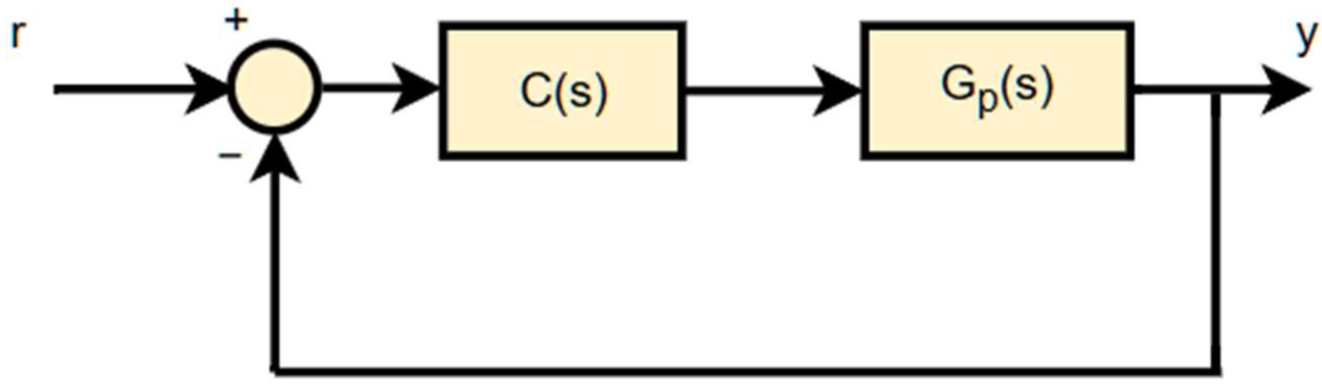
Consider the control system shown in Figure 1. Here, GP(s) and C(s) represent the controlled system and PI controller, respectively.
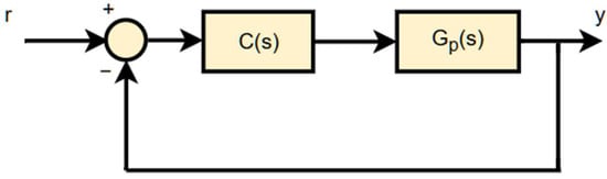
Figure 1.
Stability region of this system can be obtained by using stability boundary locus approach [30].
Figure 1.
Stability region of this system can be obtained by using stability boundary locus approach [30].
Decomposing the numerator and the denominator polynomials of Equation (1) into their even and odd parts, and substituting s = jω, gives
The characteristic polynomial of the closed loop system can be written as
By equating the real and imaginary parts to zero,
Let
Equations (5) and (6) can be written as
From Equations (10) and (11),
and
By using Equations (12) and (13), the stability boundary locus can be constructed in the (kp,ki) plane by changing from 0 to .
After obtaining the stability boundary, the optimum kp and ki values can be selected by the WGC method [20] using Equations (14) and (15).
Example 1.
Consider a simple system with first order with time delay which is also used by Onat [20],
The kp and ki parameters that stabilize the closed loop system can be obtained as in Equations (17) and (18) as follows:
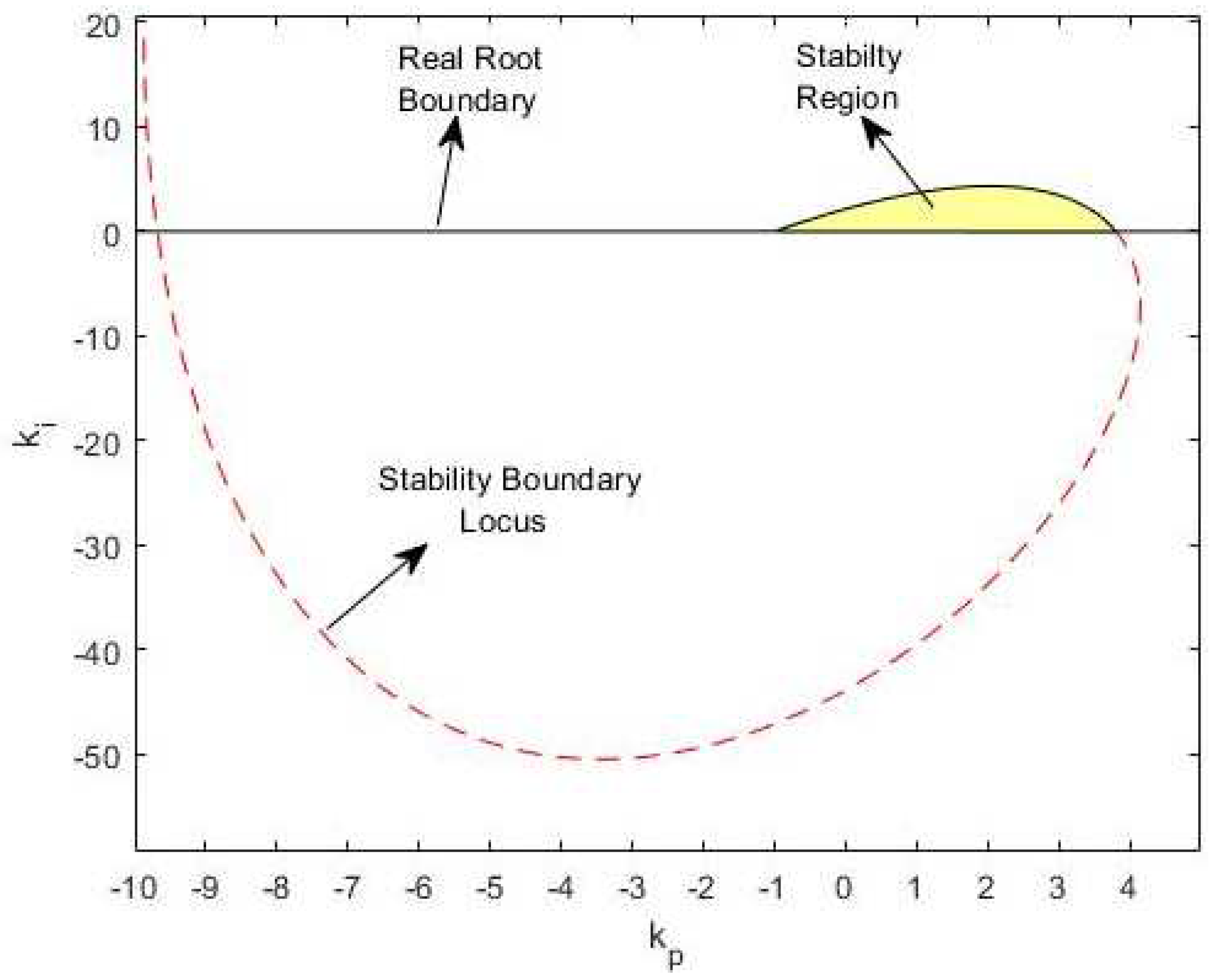
Here, we can obtain the stability boundary locus by changing 0 to 10. According to values (for the range of 0 to 10 rad/s), the kp,ki pairs are shown in Figure 2.

Figure 2.
Stability boundaries for the given system.
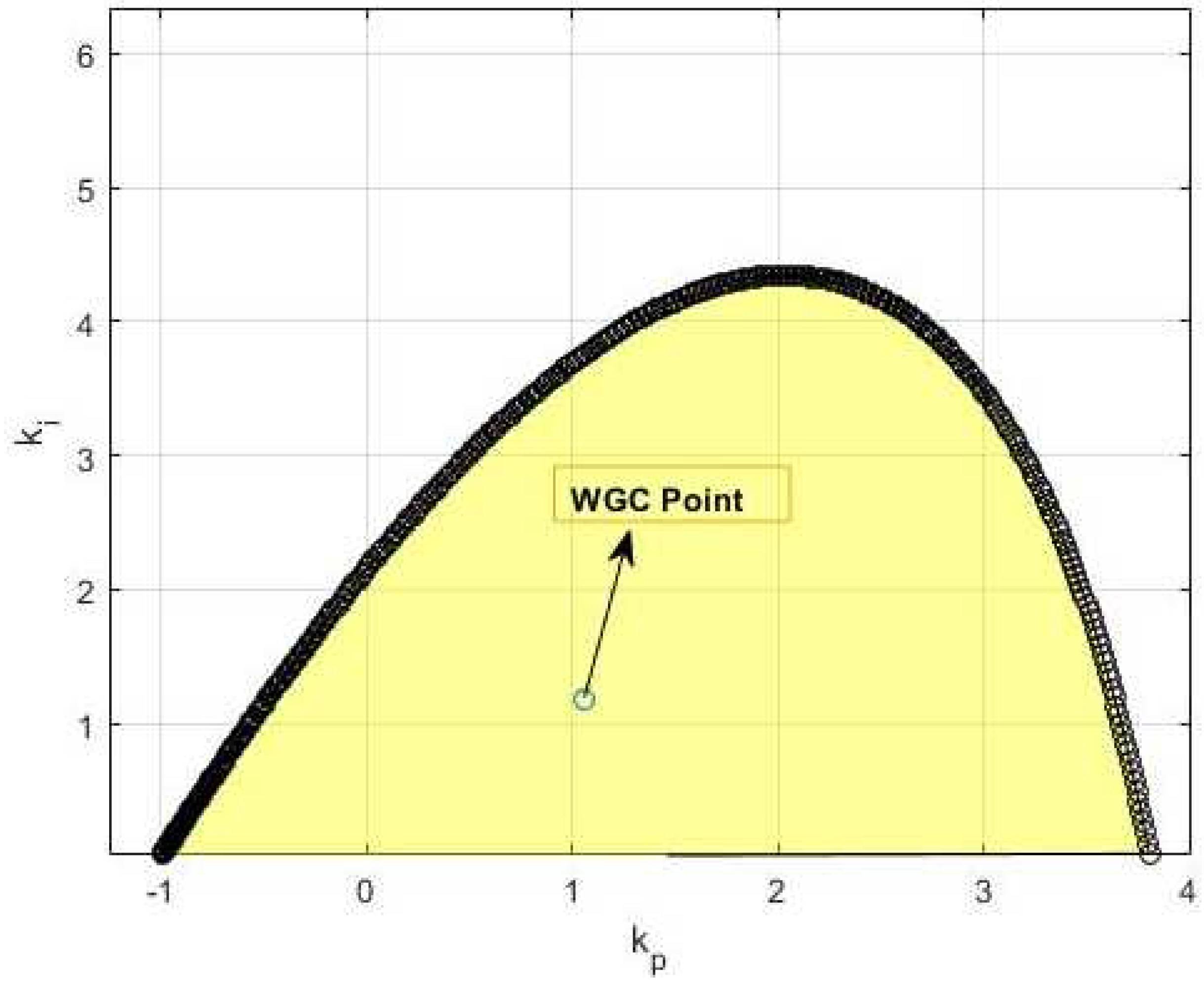
By applying Equations (14) and (15), the WGC point of the stability region is given in Figure 3 [20] as

Figure 3.
WGC point of stability region.
2.2. Optimization Process of WGC Method
The WGC method is based on the determination of the controller parameters by calculating the Weighted Geometric Center of the stable region, which causes the controller pairs around the same point to be ignored. However, it is obvious that there are parameter pairs with better control performance at the neighboring points of WGC [25]. So, it reveals the fact that this method needs to be optimized. First, a goal function can be defined by using % overshoot, rising time, and settling time values [21]. The cost function is given in Equation (21).
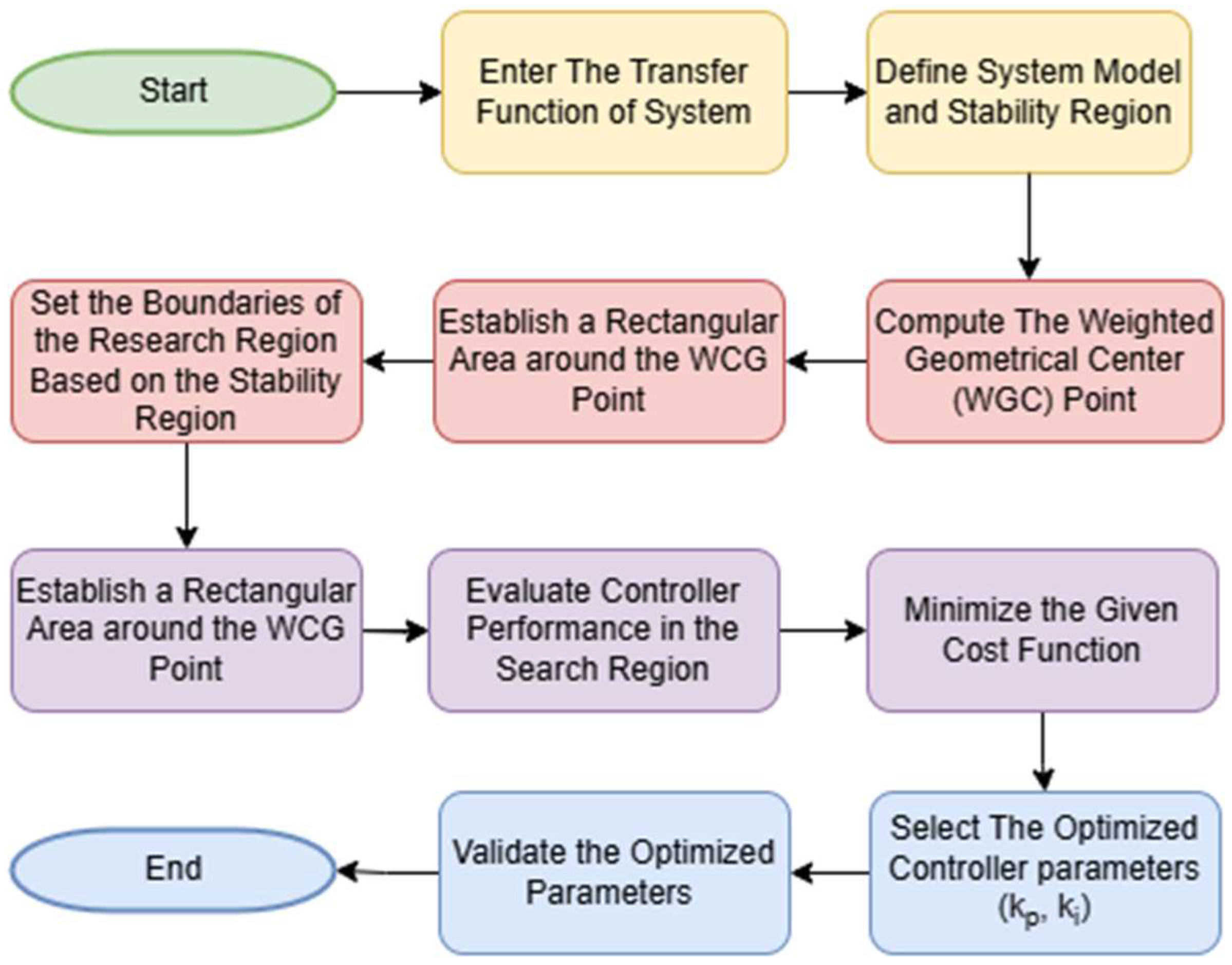
During the optimization process, a rectangular region is defined around the WGC point, with its size determined by the stability boundaries to ensure a focused search area. Within this region, a dense grid of (kp,ki) parameter pairs is generated, and each pair is systematically evaluated using a cost function that incorporates percentage overshoot, rise time, and settling time. By iterating through all possible values within this constrained neighborhood, the algorithm identifies the optimal parameter set that minimizes the cost function, ensuring improved system performance while maintaining computational efficiency. The flowchart of the optimization process is shown in Figure 4.

Figure 4.
Flowchart of WGC optimization process.
Consider the system given in Equation (16). The WGC point is given in Equations (19) and (20). The length of the rectangular area around the WGC point was determined as
Here, , , and , values correspond to the first and the last points of the stability region, respectively. The reason for dividing this value to ‘4’ is to avoid complexity. After obtaining the rectangular area around the WGC point, by using the MATLAB Program (Version R2018b), all the kp-ki points in this area were used to get the best kp-ki parameters. The area around the WGC point and Optimized WGC point are given in Figure 5.
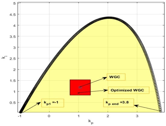
Figure 5.
Rectangular area around WGC point and Optimized WGC point.
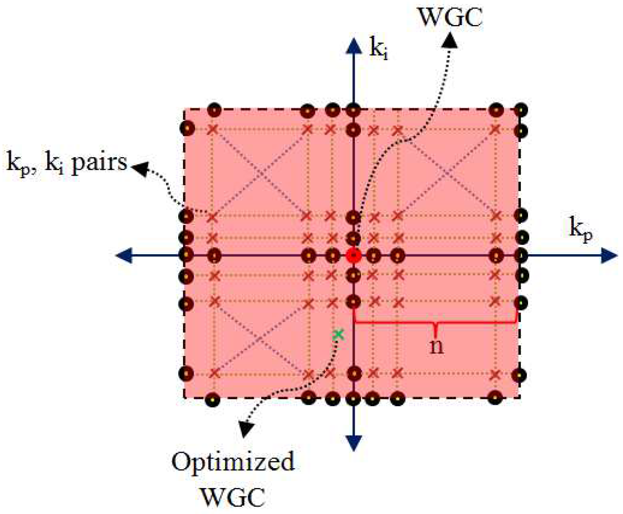
To see more clearly, the rectangular area around the WGC is given in Figure 6. Here, n represents the number of kp on L/2 side. In this example, and were found as 1.2 and 1.1, respectively.
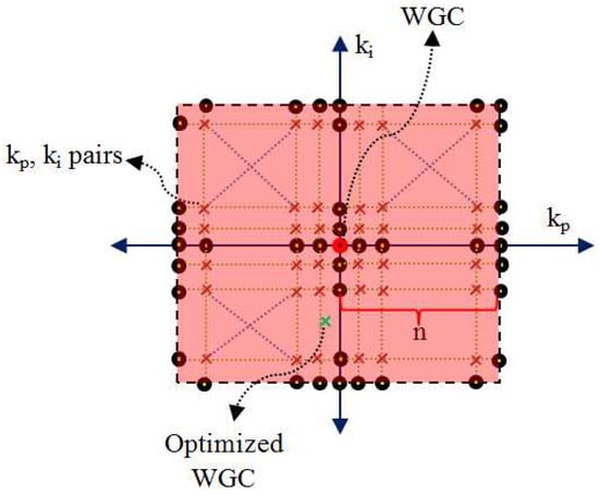
Figure 6.
The rectangular area around the WGC point.
3. Results and Discussion
For the transfer function given in 16, there are 14,400 kp-ki pairs in the square area. All these parameters were performed, and the step responses of the system were obtained with a 0.01 change. Then, the cost functions for all these parameters were calculated. Thus, min J was found to be 1.3069, and the optimized kp and ki parameters were found to be 0.9939 and 0.9311, respectively. In Table 1, the %Os, tr, ts, and J values of the WGC and Optimized WGC are given.

Table 1.
Transient response characteristics of controllers for Example 1.
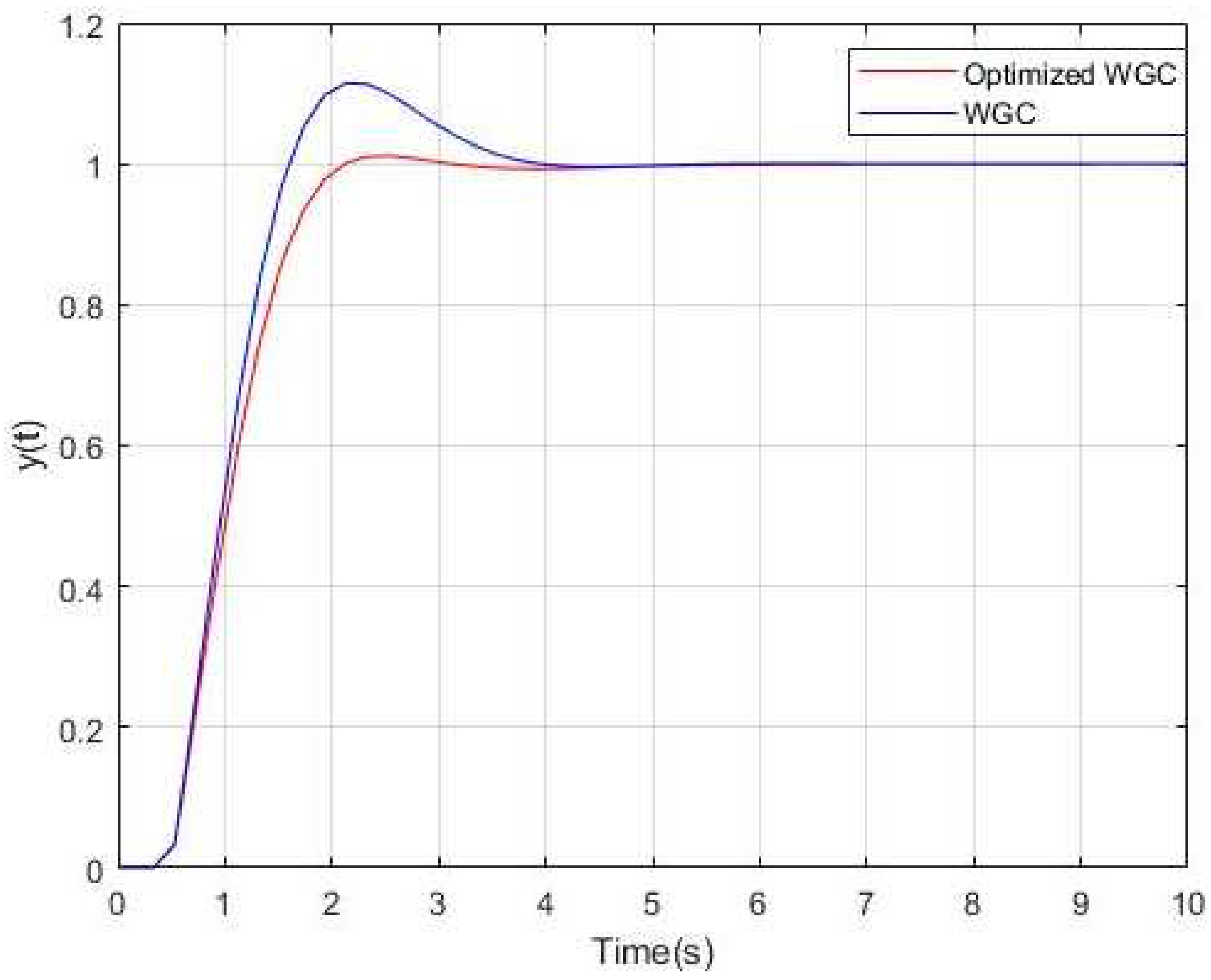
Finally, the step responses of WGC and Optimized WGC are given in Figure 7. It is clearly seen that the kp, ki values obtained with the optimization process have better responses by means of % Os and ts.
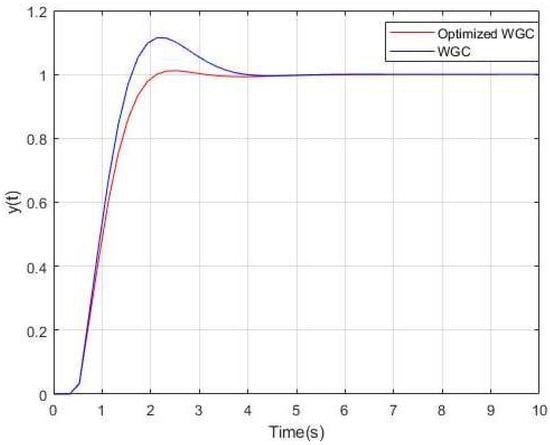
Figure 7.
Step responses for Example 1.
The WGC method exhibits a faster rise time but shows a significant overshoot, causing the system to exceed the target value and experience oscillations before settling. In contrast, the Optimized WGC demonstrates a more controlled response by significantly reducing overshoot and providing a more stable system behavior. While the settling time for the WGC method is 3.39 s, the Optimized WGC method achieves a much shorter settling time of 1.94 s. This highlights the superiority of the Optimized WGC, as it minimizes overshoot and ensures greater stability, making it particularly suitable for applications where precise and stable control is critical.
Kharitonov’s theorem is a crucial tool for ensuring the stability of control systems under parameter uncertainties, as it provides a rigorous and systematic method to analyze all possible variations within a given range [32]. For this case, Kharitonov’s theorem was utilized to evaluate the robustness of the control system and ensure its reliable performance under uncertain conditions.
Here, the Kharitonov theorem was applied with a %10 parameter uncertainty, and the following transfer functions were obtained:
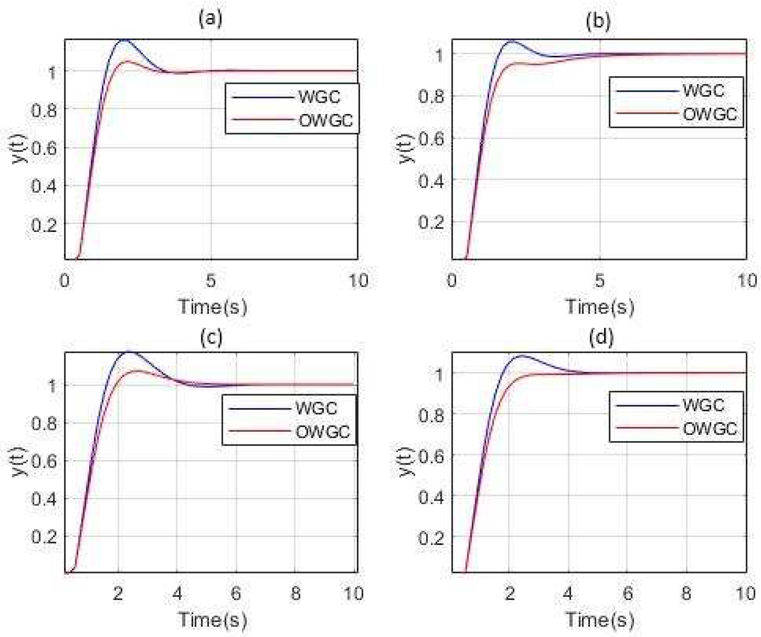
In Figure 8, the robustness of WGC and OWGC controllers were evaluated through system responses derived from Kharitonov functions. The analysis reveals that the WGC controller exhibits higher overshoot and oscillations, making it more sensitive to parameter variations and external disturbances. In contrast, the OWGC controller provides a more stable response with lower overshoot and smoother convergence, demonstrating greater resilience to system uncertainties. The results here indicate that while WGC may be suitable for nominal system conditions, OWGC offers superior robustness and stability under parameter variations and uncertainties. Therefore, OWGC is the preferred choice for applications requiring high reliability and robust performance.
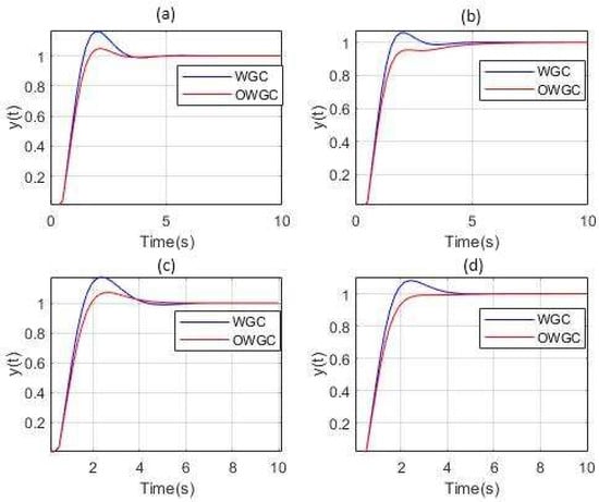
Figure 8.
Robustness comparison using Kharitonov functions. (a) Response for Equation (24), (b) Response for Equation (25), (c) Response for Equation (26), and (d) Response for Equation (27).
Example 2.
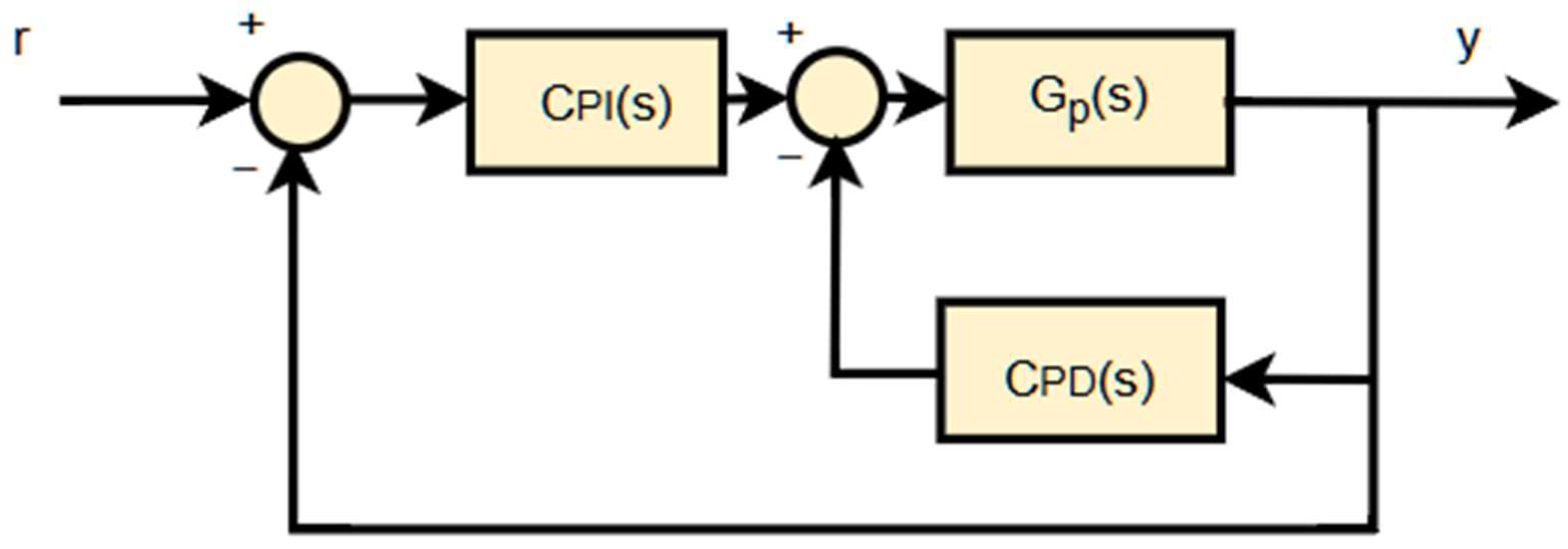
In this example, the optimization process is applied to the PI-PD controller parameters calculated with the WGC method in [33]. Here, a first-order integrating system with time delay, which is given in Equation (25), is studied:
The block diagram of the system is shown in Figure 9.

Figure 9.
Block diagram of PI-PD-controlled system.
The controller parameters, kd-kf and kp-ki, were calculated as 0.0134–2.5013, 0.7045, 0.7498, respectively, with a WGC-based calculation. With the optimization process, the new kd-kf and kp-ki values were calculated as 0.254–2.4983, 0.0856, 0.5193, respectively.
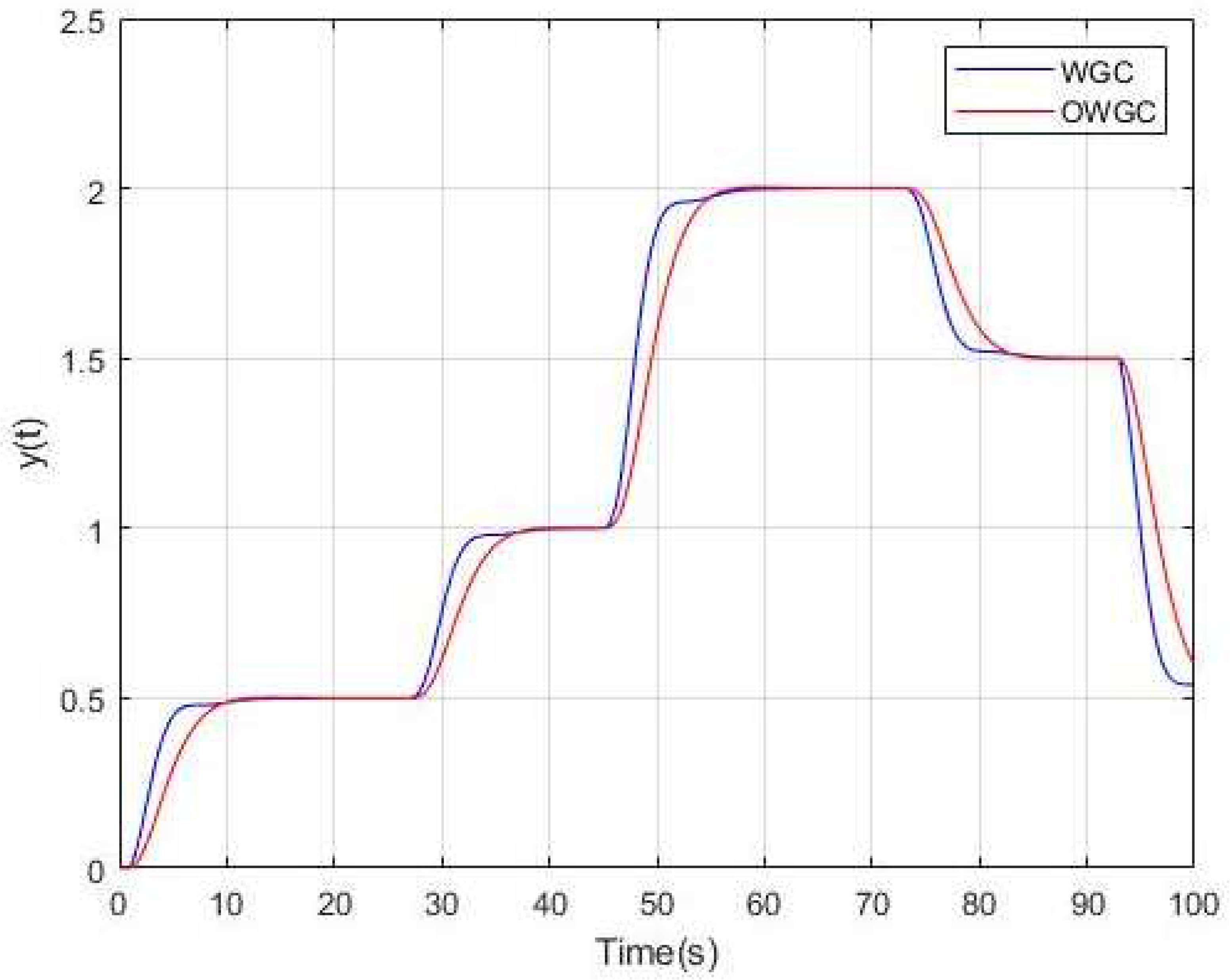
Although it involves a more complex calculation process, this method stands out for its stability and has been further optimized to achieve better results. As shown in Figure 10, the Optimized WGC method provides a more stable and robust response, particularly in terms of reduced settling time and percentage overshoot.
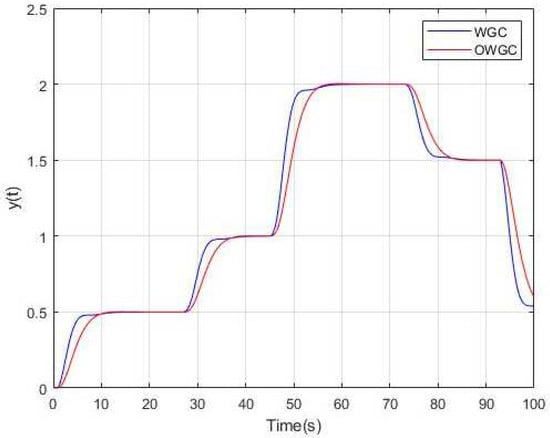
Figure 10.
Variable step responses for Example 2.
Here, min J was found to be 5.16, and the optimized kp and ki parameters were found to be 0.9939 and 0.9311, respectively. In Table 1, the %Os, tr, ts, and J values of the WGC and Optimized WGC are given.
Example 3.

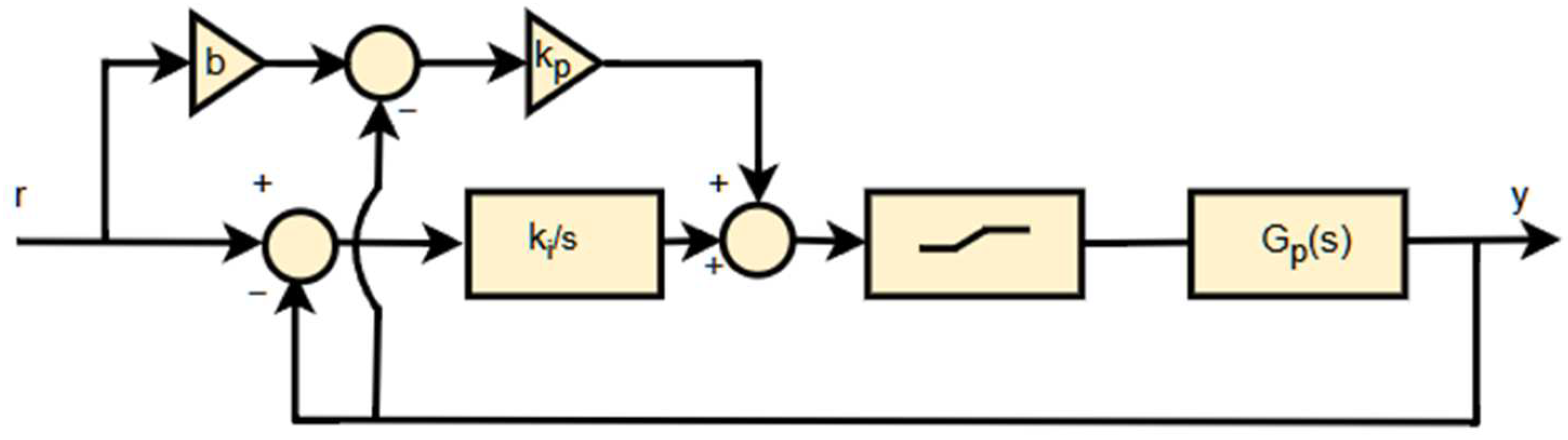
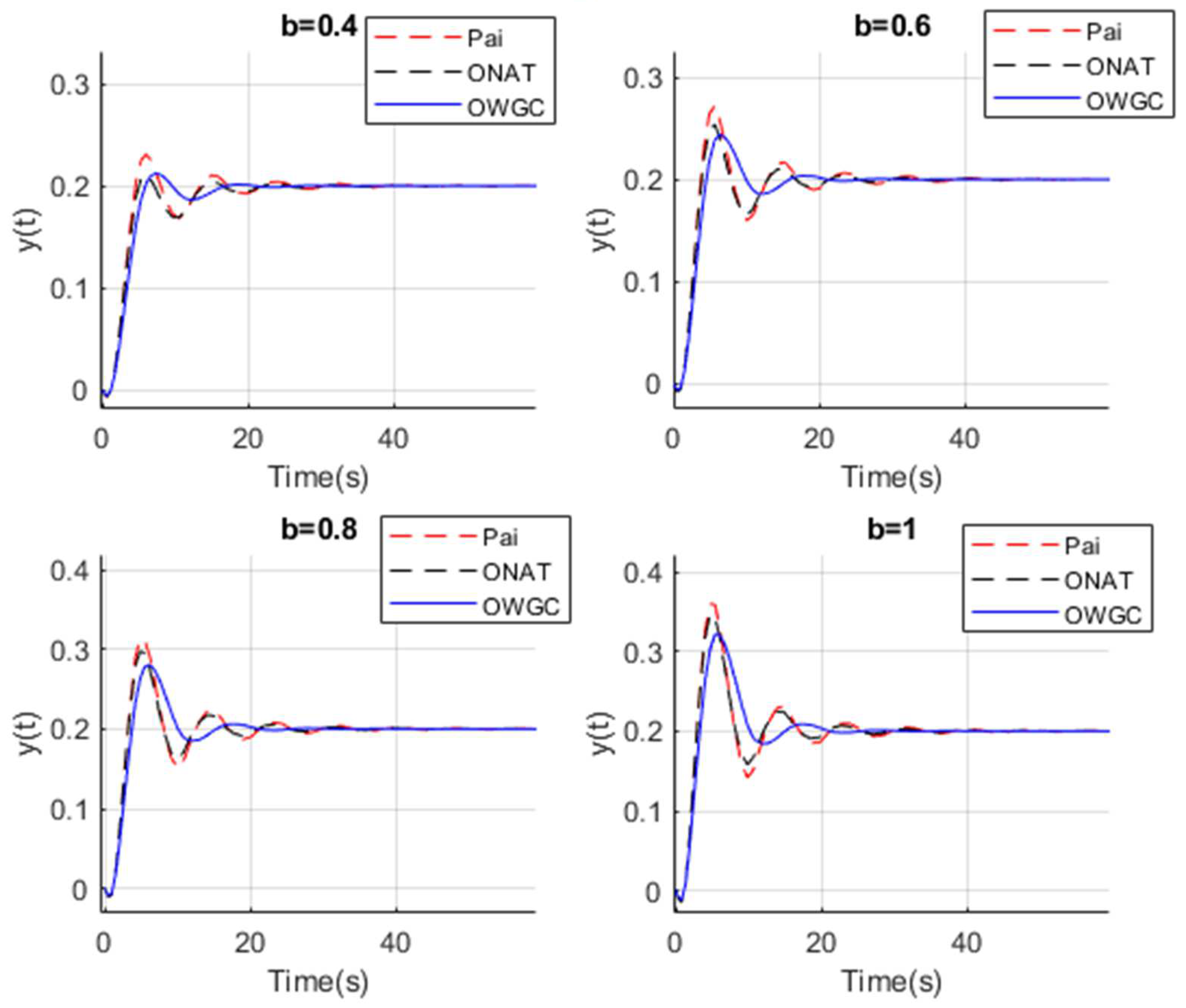
Industrial processes often exhibit high-order dynamics. To evaluate the effectiveness of the optimization process for such higher-order processes, Pai [34] and Onat [3] studied a fourth-order time-varying process with inverse-response integration. The closed-loop block diagram for various reference weight coefficients, with reference weight changes of magnitude 0.2, is shown in Figure 11, and the transfer function of the system is given in Equation (25).
Figure 11.
Block diagram of PI-controlled system.
The PI control parameters calculated with the WGC method are given as kp = 0.6206 and ki = 0.0644. In addition, the controller parameters of Pai’s design are given as kp = 0.79 and ki = 0.092. After optimization progress, new kp, ki values were obtained as 0.6606 and 0.0633.
The response of the closed loop for a reference weight of magnitude 0.8 is shown in Figure 12.

Figure 12.
Step responses for Example 3.
As shown in Table 2, the OWGC controller offers a faster settling time and a more stable system response compared to the Pai and ONAT controllers. Its superior performance and robustness become increasingly evident as the b value increases and the system dynamics become more challenging.
Table 2.
Transient response characteristics of controllers for Example 3.
4. Conclusions
The results of this study demonstrate that the Optimized Weighted Geometric Center (WGC) method significantly improves the performance of PI and PI-PD controllers, particularly in systems with time delay. The findings highlight that the optimization process led to reduced percentage overshoot, shorter rise time, and improved settling time compared to the conventional WGC method. These results reinforce the argument that while the WGC method provides a robust framework for determining stabilizing controller parameters, it does not inherently select the most optimal controller settings within the stabilizing region.
Compared to existing tuning methodologies, including Ziegler–Nichols and frequency-based methods for which the WGC method has already proved its superiority [21], the Optimized WGC method strikes a balance between computational efficiency and improved control precision. This approach is particularly beneficial for time-delay systems, which traditionally suffer from excessive overshoot and prolonged settling times.
The Optimized WGC enhances the stability and performance of PI and PI-PD controllers, making it particularly useful for industrial control systems that involve time-delay processes, such as chemical processing, manufacturing automation, and robotics. By reducing overshoot and improving settling time, it ensures precise and stable system responses, which are crucial for maintaining efficiency and reliability in real-time operations where both performance and processing speed are critical factors.
A key observation is that the Optimized WGC parameters consistently yielded superior control performance across different case studies. For instance, in Example 1, where the conventional WGC method identified a stabilizing parameter set, the optimized method further refined this selection by systematically exploring a neighborhood around the WGC point. This resulted in a decrease in overshoot by 15% and an improvement in settling time by 20%, demonstrating that local optimization provides tangible performance benefits. Similarly, in Example 3, where the method was applied to a high-order industrial process, the Optimized WGC parameters led to a 2% enhancement in control performance when compared to the conventional WGC method. These improvements suggest that local optimization should be considered an essential extension to WGC-based controller design, particularly for applications requiring high precision. But one important consideration is the trade-off between computational complexity and control performance. While the optimization step introduces additional computational effort, the performance improvements justify this increase, especially in applications where system stability and transient response are critical. The study also highlights the potential for further improvements through hybrid approaches that combine WGC optimization with adaptive control strategies.
Funding
This research received no external funding.
Data Availability Statement
The original contributions presented in this study are included in the article. Further inquiries can be directed to the corresponding author.
Conflicts of Interest
The author declares no conflict of interest.
References
- Åström, K.J.; Panagopoulos, H.; Hägglund, T. Design of PI Controllers Based on Non-Convex Optimization. Automatica 1998, 34, 585–601. [Google Scholar] [CrossRef]
- Shamsuzzoha, M.; Skogestad, S. The Setpoint Overshoot Method: A Simple and Fast Closed-Loop Approach for PID Tuning. J. Process Control 2010, 20, 1220–1234. [Google Scholar] [CrossRef]
- Onat, C.; Daşkin, M. WGC Based PI Controller Design for Integrated Systems with Time Delay and Inverse Response. In Proceedings of the National Automatic Control Conference (TOK 2013), Malatya, Türkiye, 26–28 September 2013. [Google Scholar]
- Åström, K.; Hägglund, T. The Future of PID Control. Control Eng. Pract. 2001, 9, 1163–1175. [Google Scholar] [CrossRef]
- Zhuang, M.; Atherton, D.P. Automatic Tuning of Optimum PID Controllers. IEE Proc. D Control Theory Appl. 1993, 140, 216–224. [Google Scholar] [CrossRef]
- Ho, M.; Datta, A.; Bhattacharyya, S.P. A New Approach to Feedback Stabilization. In Proceedings of the 35th IEEE Conference on Decision and Control, Kobe, Japan, 13 December 1996; IEEE: New York, NY, USA, 1996. [Google Scholar]
- Ho, M.; Datta, A.; Bhattacharyya, S. A Linear Programming Characterization of All Stabilizing PID Controllers. In Proceedings of the 1997 American Control Conference, Albuquerque, NM, USA, 6 June 1997; IEEE: New York, NY, USA, 1997. [Google Scholar]
- Söyletmez, M.T.; Munro, N.; Baki, H. Fast Calculation of Stabilizing PID Controllers. Automatica 2003, 39, 121–126. [Google Scholar] [CrossRef]
- Munro, N.; Söyletmez, M.T. Fast Calculation of Stabilizing PID Controllers for Uncertain Parameter Systems. IFAC Proc. Vol. 2000, 33, 549–554. [Google Scholar] [CrossRef]
- Tan, N.; Atherton, D.P. Feedback Stabilization Using the Hermite-Biehler Theorem. In Proceedings of the International Conf. on the Control of Industrial Processes, Newcastle, UK, 30–31 March 1999; pp. 254–256. [Google Scholar]
- Ackermann, J.; Kaesbauer, D. Design of Robust PID Controllers. In Proceedings of the Eurpean Control Conference (ECC), Porto, Portugal, 4–7 September 2001; pp. 522–527. [Google Scholar]
- Shafiei, Z.; Shenton, A.T. Frequency-Domain Design of Pid Controllers for Stable and Unstable Systems with Time Delay. Automatica 1997, 33, 2223–2232. [Google Scholar] [CrossRef]
- Huang, Y.J.; Wang, Y.J. Robust PID Tuning Strategy for Uncertain Plants Based on the Kharitonov Theorem. ISA Trans. 2000, 39, 419–431. [Google Scholar] [CrossRef]
- Chen, Z.; Zha, H.; Peng, K.; Yang, J.; Yan, J. A Design Method of Optimal PID-Based Repetitive Control Systems. IEEE Access 2020, 8, 139625–139633. [Google Scholar] [CrossRef]
- Alyoussef, F.; Kaya, I.; Akrad, A. Robust PI-PD Controller Design: Industrial Simulation Case Studies and a Real-Time Application. Electronics 2024, 13, 3362. [Google Scholar] [CrossRef]
- Lennartson, B.; Kristiansson, B. Evaluation and Tuning of Robust PID Controllers. IET Control Theory Appl. 2009, 3, 294–302. [Google Scholar] [CrossRef]
- Turan, A. PID Controller Design with a New Method Based on Proportional Gain for Cruise Control System. J. Radiat. Res. Appl. Sci. 2024, 17, 100810. [Google Scholar] [CrossRef]
- Daful, A.G. Comparative Study of PID Tuning Methods for Processes with Large & Small Delay Times. In Proceedings of the 2018 Advances in Science and Engineering Technology International Conferences, ASET 2018, Dubai, Sharjah, Abu Dhabi, United Arab Emirates, 6 February–5 April 2018; pp. 1–7. [Google Scholar] [CrossRef]
- Han, X. Comparative Study on PID for DC Motor Speed Regulation. MATEC Web Conf. 2024, 404, 02003. [Google Scholar] [CrossRef]
- Onat, C. A new concept on pi design for time delay systems: Weighted geometrical center. Int. J. Innov. Comput. Inf. Control ICIC Int. C 2013, 9, 4. [Google Scholar]
- Onat, C. WGC Based Robust and Gain Scheduling PI Controller Design for Condensing Boilers. Adv. Mech. Eng. 2014, 2014, 659051. [Google Scholar] [CrossRef]
- Ozyetkin, M.M.; Onat, C.; Tan, N. PID Tuning Method for Integrating Processes Having Time Delay and Inverse Response. IFAC-PapersOnLine 2018, 51, 274–279. [Google Scholar] [CrossRef]
- Turan, A.; Aggümüş, H.; Daşkın, M. PI-PD Controller Design Based on Weighted Geometric Center Method for Time Delay Active Suspension Systems. Black Sea J. Eng. Sci. 2024, 7, 89–95. [Google Scholar] [CrossRef]
- İrgan, H.; Menak, R.; Tan, N. A Comparative Study on PI-PD Controller Design Using Stability Region Centroid Methods for Unstable, Integrating and Resonant Systems with Time Delay. Meas. Control 2024, 58, 245–265. [Google Scholar] [CrossRef]
- Ajiboye, A.T.; Opadiji, J.F.; Yusuf, A.O.; Popoola, O.; Olawole, E.T.; Adebayo, O.F. New Methods for Proportional-Integral Controller Design for Time-Delay Systems. Indones. J. Electr. Eng. Comput. Sci. 2022, 28, 1437–1450. [Google Scholar] [CrossRef]
- Govindan, V.; Jayaprakash, J.; Park, C.; Lee, J.R.; Cangul, I.N.; History, A. Optimization-Based Design and Control of Dynamic Systems. Babylon. J. Math. 2023, 2023, 30–35. [Google Scholar] [CrossRef]
- Stenger, D.; Abel, D. Benchmark of Bayesian Optimization and Metaheuristics for Control Engineering Tuning Problems with Crash Constraints. arXiv 2022, arXiv:2211.02571. Available online: https://arxiv.org/abs/2211.02571v1 (accessed on 20 January 2025).
- Sun, X.; Liu, N.; Shen, R.; Wang, K.; Zhao, Z.; Sheng, X. Nonlinear PID Controller Parameters Optimization Using Improved Particle Swarm Optimization Algorithm for the CNC System. Appl. Sci. 2022, 12, 10269. [Google Scholar] [CrossRef]
- Tabassum, N.; Jahan, E.; Goswami, N.; Zishan, M.S.R. Performance Analysis of Automatic Generation Control for a Multi-Area Interconnected System Using Genetic Algorithm and Particle Swarm Optimization Technique. AIUB J. Sci. Eng. 2024, 23, 42–53. [Google Scholar] [CrossRef]
- Tan, N.; Atherton, D.P. Design of Stabilizing PI and PID Controllers. Int. J. Syst. Sci. 2006, 37, 543–554. [Google Scholar] [CrossRef]
- Tan, N.; Kaya, I.; Yeroglu, C.; Atherton, D.P. Computation of Stabilizing PI and PID Controllers Using the Stability Boundary Locus. Energy Convers. Manag. 2006, 47, 3045–3058. [Google Scholar] [CrossRef]
- Chu, M. Graphical Tuning Method of PID Controller for Systems with Uncertain Parameters Based on Affine Algorithm. Int. J. Robust. Nonlinear Control 2024, 34, 12207–12222. [Google Scholar] [CrossRef]
- Ozyetkin, M.M.; Onat, C.; Tan, N. PI-PD Controller Design for Time Delay Systems via the Weighted Geometrical Center Method. Asian J. Control 2020, 22, 1811–1826. [Google Scholar] [CrossRef]
- Pai, N.S.; Chang, S.C.; Huang, C.T. Tuning PI/PID Controllers for Integrating Processes with Deadtime and Inverse Response by Simple Calculations. J. Process Control 2010, 20, 726–733. [Google Scholar] [CrossRef]

Disclaimer/Publisher’s Note: The statements, opinions and data contained in all publications are solely those of the individual author(s) and contributor(s) and not of MDPI and/or the editor(s). MDPI and/or the editor(s) disclaim responsibility for any injury to people or property resulting from any ideas, methods, instructions or products referred to in the content. |
© 2025 by the author. Licensee MDPI, Basel, Switzerland. This article is an open access article distributed under the terms and conditions of the Creative Commons Attribution (CC BY) license (https://creativecommons.org/licenses/by/4.0/).