A Deep Reinforcement Learning-Based Evolutionary Algorithm for Distributed Heterogeneous Green Hybrid Flowshop Scheduling

Abstract

Due to increasing energy consumption, green scheduling in the manufacturing industry has attracted great attention. In distributed manufacturing involving heterogeneous plants, accounting for complex work sequences and energy consumption poses a major challenge. To address distributed heterogeneous green hybrid flowshop scheduling (DHGHFSP) while optimising total weighted delay (TWD) and total energy consumption (TEC), a deep reinforcement learning-based evolutionary algorithm (DRLBEA) is proposed in this article. In the DRLBEA, a problem-based hybrid heuristic initialization with random-sized population is designed to generate a desirable initial solution. A bi-population evolutionary algorithm with global search and local search is used to obtain the elite archive. Moreover, a distributional Deep Q-Network (DQN) is trained to select the best local search strategy. Experimental results on 20 instances show a 9.8% increase in HV mean value and a 35.6% increase in IGD mean value over the state-of-the-art method. The results show the effectiveness and efficiency of the DRLBEA in solving DHGHFSP.

1. Introduction

The advancement of automation technology has led to a significant expansion in the the modern industrial sector‘s production potential. The scheduling of production processes represents a pivotal decision-making challenge in manufacturing systems [1] and is a subject of extensive study. The flowshop scheduling problems (FSPs), such as the no-wait flowshop [2], hybrid flowshop [3,4], distributed flowshop [5] problems, etc., are classic problems in scheduling problems. To quickly adapt to market demands and shorten production lead times, components for large-scale equipment are often allocated to multiple factories for simultaneous manufacturing. Distributed manufacturing enables the production of high-quality products at lower costs and reduced risks, which is more relevant to the actual production.

The distributed hybrid flowshop scheduling problem (DHFSP) is a complex production scheduling problem that combines the characteristics of the hybrid flowshop scheduling problem (HFSP) and distributed production systems [6]. A significant challenge arises from the necessity of coordinating the production schedule of each shop in a distributed environment. This entails the consideration of factory allocation, which can be represented by the addition of a vector. This design is more aligned with the complexities of real-world production. However, due to the inherent variability of actual production processes and the differences in production methods across machines, each factory is characterised by a unique set of circumstances. This results in a distributed heterogeneous hybrid flowshop scheduling problem (DHHFSP) [7]. The expanded decision space renders it more complex to resolve than the standard DHFSP. The DHHFSP necessitates the concurrent optimisation of job processing sequences, machine assignments, and plant allocations.

In light of the advancements made in the field of sustainable development, environmental protection has emerged as a critical consideration in industrial production [8]. It is inevitable that a considerable amount of energy will be consumed during the manufacturing process, with the inevitable consequence that non-renewable resources will be depleted. The distribution of machinery in a factory setting is not uniform and may be subject to different processing techniques. Consequently, it is vital for the manufacturing industry as a whole to develop effective scheduling strategies and to improve existing technologies in order to reduce total energy consumption [9]. The distributed heterogeneous hybrid flowshop scheduling problem (DHGHFSP) is a DHHFSP that considers energy saving.

The DHGHFSP can be elaborated as follows: Multiple jobs need to be processed within factories that are geographically dispersed. Each factory boasts a certain number of stages, each stage has some parallel machines capable of handling the tasks that can process one job at a time. Each job has a due date and priority. The scheduling objective, subject to various constraints such as operation sequence, machine capacity, and processing time constraints, is to optimise one or more performance metrics. These metrics typically include makespan, total energy consumption, and total weight delay. The DHHFSP is an NP-hard problem as a expansion of the HFSP [10], and it is difficult to solve this problem through simple analytical methods. Researchers have proposed a variety of approaches to solve these problems include tabu search [11], NSGA-II [12], iterative local search [7], and iterative greedy search, among others.

The DHGHFSP is a problem which has a heterogeneous factory environment and a complex scheduling environment that require a more effective approach. Reinforcement Learning (RL) is an effective method for learning and controlling complex and uncertain environments. The goal of RL is to maximize the cumulative rewards gained by an intelligent body during interaction with its environment [13]. RL comprises five principles: (1) input and output systems; (2) rewards; (3) artificial intelligence environment; (4) Markov Decision Process (MDP); (5) training and inference. Value-based reinforcement learning focuses on estimating the value of each state or state–action pair to select the action that yields the highest reward in each state, thus indirectly determining the optimal policy. In this study, a deep reinforcement learning is used to choose the best local search strategies, and a distributional DQN is used to estimate the Q-value distribution of the current state–action.

In this study, a deep reinforcement learning-based evolutionary algorithm (DRLBEA) is proposed to solve the DHGHFSP. To solve the large-scale scheduling problem, this article introduces a distributional DQN-based evolutionary algorithm. Our contributions are as follows:

(1) Considering real-world production scheduling, this study addresses the problem of plant heterogeneity in the DHFSP. It addresses the constraints in time production by recognising that each plant may have different processing times and each job has a deadline completion date and priority

(2) A genetic algorithm was chosen, combined with local search based on problem features to form the overall framework. A multi-population initialization is designed which has different equal-sized subpopulations (Section 4.5) which enhance the initial solution.

(3) This research utilizes a distributional DQN-based algorithm to choose the best operator for the local search by interacting with the environment and updating weights to estimate the Q-value distribution of the current state–action. Unlike traditional DQN, which calculates the Q-value for each action separately, distributional DQN splits the Q-value into two parts: the state-value function $V(s,z)$, representing the overall value of a state; and the advantage function $A(s,a,z)$, which quantifies the advantage of each action relative to the state.

The remainder of the article is organized as follows. Section 3 introduces the concept of DHGHFSP. Section 4 describes the framework and details of the DRLBEA. Section 5 presents the experimental data and analysis. Section 6 summarizes the full paper and suggests directions for future research.

2. Literature Review

For solving scheduling problem, heuristic algorithms are mostly currently employed [14]. The FSP, as the basic issue, has a different expansion. In [15], a Q-learning algorithm is designed to adaptively adjust the selection probabilities of four key population update strategies in the classic Aquila optimiser which do well in improving the performance of the Aquila optimiser but do not consider the exploration and exploitation period in the Aquila optimiser. In [2], a two-stage cooperative evolutionary algorithm with problem-specific knowledge called TS-CEA is proposed to address the energy-efficient scheduling of the no-wait flowshop problem (EENWFSP) with the criteria of minimizing both makespan and total energy consumption which is effective at designing the initialization method but is limited by application scenarios.

As for the HFSP, Janis et al. provided a detailed review of the multiobjective HFSP [4], presenting a systematisation of performance criteria for evaluating the Pareto front. In [3], an energy-aware multiobjective optimisation algorithm (EA-MOA) was proposed, which designed various neighbourhood structures and adaptive neighbourhood selection and had good robustness and effectiveness but lacked local search capabilities. Fan et al. applied a hybrid evolutionary algorithm (HEA) using two solution representations; using a tabu search (TS) process based on a disjunctive graph representation to expand the search space, that method better balanced the optimality and efficiency but tended to be time-consuming in solving large-scale instances [11]. Considering an uncertain situation in the energy-efficient HFSP, Wang extended the Existing Nondominated Sorting Genetic Algorithm-II (ENSGA-II) to address the energy-efficient fuzzy HFSP with variable machine speeds; ENSGA-II had powerful parameter adjustment strategy and a novel historical information utilization method but lacked in interruption and pre-emption [12].

Regarding the DHFSP, Wang considered a bi-population cooperative memetic algorithm (BCMA) and designed two knowledge-based heuristics to overcome; the BCMA could balance global exploration and local exploitation but was weak in solving other types of distributed scheduling problems [16]. Zheng addressed a multiobjective fuzzy DHFSP with fuzzy processing times and fuzzy due dates, and a co-evolutionary algorithm with problem-specific strategies was proposed by rationally combining the Estimation of Distribution Algorithm (EDA) and Iterative Greedy Search (IG). The model balanced exploration and exploitation of the algorithm, but it was difficult to solve scheduling problems with uncertainties [17]. Zhang et al. dealt with a distributed hybrid differentiation flowshop problem (DHDFSP), proposing a distributed co-evolutionary memetic algorithm (DCMA); DCMA had a superior architecture as well as well-designed modules but was weak in multiobjective and heterogeneous scenarios [18]. In [19], Zhang presented an archive-assisted adaptive memetic algorithm (EAMA) to solve the DHDFSP which had an excellent architecture and components, but it was hard to cope with more realistic DHFSPs. Wang proposed a cooperative memetic algorithm (CMA) with a reinforcement learning (RL)-based policy agent; that method’s enhanced search combining multi-problem operators had a high search capability; however, the disadvantage of the CMA was solving other types of energy-aware distributed scheduling problems [20].

Concerning the DHHFSP, Chen et al. investigated a distributed heterogeneous hybrid flowshop scheduling problem with lot-streaming (DHHFSPLS) and established a knowledge-driven many-objective optimisation evolutionary algorithm (KDMaOEA), which was strong in exploitation abilities and helped the algorithm optimise each objective sufficiently but lacked any consideration of costs and uncertainties [7]. Qin et al. studied a mathematical model of the DHHFSP with blocking constraints and designed a collaborative iterative greedy (CIG) algorithm; the local intensification strategy was developed to optimise the scheduling sequence of each factory, but CIG did not consider the adjustment of the number of jobs in the factory after the factory was allocated to the jobs [21]. Under nonidentical time-of-use electricity tariffs, Shao et al. proposed an ant colony optimisation behaviour-based multiobjective evolutionary algorithm based on decomposition, using a problem-specific ant colony behaviour to construct offspring individuals; the method performed well in energy saving, but the contribution of the global search was not enough [22].

Nowadays, reinforcement learning is widely used and can be applied to a variety of problems. In [20], a reinforcement learning-based policy agent was used to select solutions with appropriate improvement operator. In [23], a deep reinforcement learning was used for solving the re-entrant hybrid flowshop scheduling problem with stockers (RHFS2). In this study, the states, actions, and rewards of the Markov decision process for this problem are designed, and two deep Q-network (DQN) approaches based on the actions for determining machines and jobs, respectively, are proposed. Li et al. proposed a deep Q-network-based co-evolution algorithm which were applied to learn and select the best operator for each solution [24].

Table 1. Methods in the literature review.

Problem	Method	Advantage	Disadvantage
HFSP	EA-MOA	Good robustness and effectiveness	Local search capabilities
	HEA	Balances the optimality and efficiency	Time-consuming when solving large-scale instances
	ENSGA-II	Powerful parameter adjustment	Interruption and pre-emption
DHFSP	BCMA	Balances global search and local search	Solving other distributed scheduling problems
	CCA	Balances exploration and exploitation	Hard to solve scheduling problems with uncertainties
	DCMA	Architecture and modules	Multiobjective and heterogeneous scenarios
	EAMA	Excellent architecture and components	More realistic DHFSP
	CMA	Enhances search operators	Other energy-aware DHFSP
DHHFSP	KDMaOEA	Exploitation ability	Costs and uncertainties
	CIG	Local intensification strategy	Adjustment of jobs
	ACO_MOEA/D	Energy saving	Global search

shows the methods of these literature and their advantages and disadvantages.

3. Problem Description and Mathematical Model

3.1. Problem Description

The DHGHFSP is similar to the DHFSP, however, in the DHGHFSP, the composition varies from plant to plant. There are n jobs that need to be assigned to $n_f$ factories, and each factory possesses t stages and $m_t$ parallel machines. Specifically, each job has a due date $D_i$ and a priority $R_i$ Each job should be completed before $D_i$. The lower the $R_i$, the more important and urgent the job. There are three issues to consider in this model: (1) Job allocation to a specific factory, (2) parallel machine selection at every stage for each job, (3) processing order across all heterogeneous factories. In addition, the conditions of the DHGHFSP are shown bellow:

(1) Each concurrent unit is capable of handling only a single task simultaneously.

(2) A job should be allocated to one factory only.

(3) These heterogeneous factories have different processing times at each stage for different jobs.

(4) All machines are available at time 0.

(5) The setup time and dynamic events are disregarded.

3.2. MILP Model for DHGHFSP

The notation is described in

Table 2. Notation of DHGHFSP.

Type	Symbol	Definition
Index	i	Index of the job; $i=1,2,\dots ,n$
	f	Index of the factory; $f=1,2,\dots ,F$
	S	Index of the stage; $s=1,2,\dots ,S$
	k	Index of the machine; $k=1,2,\dots ,m$
	t	Index of the position; $t=1,2,\dots ,T$
Parameter	n	Number of jobs
	F	Number of factories
	S	Number of stages for each factory
	m	Number of machines in each factory
	T	Number of positions for each machine
	L	A large positive number
	$E_{idle}$	Energy consumption of idle time
	$E_{pro}$	Energy consumption of processing time
	$D_i$	Deadline of job i
	$R_i$	Priority of job i; $R_i\in \{1,2,3\}$
	$P_{f,i,s}$	The duration required for job i during stage s at factory f
	${\gamma }_{R_i}$	Punishment factor; for each $R_i$, ${\gamma }_{R_i}\in \{2.5,1.5,1\}$
Variable	$S{T}_{f,i,s}$	The initiation timestamp of job i during stage s at factory f
	$F{T}_{f,i,s}$	The completion timestamp of job i during s at factory f
	$B{T}_{f,s,k,t}$	The start time of machine $M_{f,s,k}$ during stage s at position t in factory f
	$E{C}_{f,s,k,t}$	The idle energy consumption on machine $M_{f,s,k}$ during stage s at position t in factory f
	$V_i$	The deadline violation of job i; $V_i=max(F{T}_{f,i,S}-D_i,0)$
	$X_{f,i}$	1 if job i is allocated to factory f and 0 otherwise
	$Y_{f,s,k,i,t}$	1 if job i is processed at position t of machine $M_{f,s,k}$ during stage s in factory f, and 0 otherwise.

.

The DHGHFSP is considered to minimize two conflicting objectives, including total weighted delay (TWD) [25] and total energy consumption (TEC), elaborated as follows:

(1) Total energy consumption: include the energy consumption of processing time and idle time.

$$\begin{array}{c}\hfill TEC=\sum _{f=0}^F\sum _{i=0}^N\sum _{s=0}^S{X}_{f,j}\ast P_{f,i,s}\ast E_{pro}+\sum _{f=0}^F\sum _{s=0}^S\sum _{k=0}^M\sum _{t=0}^M{E}_{f,s,k,t}\end{array}$$

(1)

(2) Total weighted delay: this reflect the income of the factory; a smaller $TWD$ means all orders are better fulfilled and priority and expiry data limits are better balanced.

$$TWD=\sum _{i=0}^{N-1}max(0,V_i)\ast {\gamma }_{R_i}$$

(2)

The MILP model can be defined as:

$$\left\{\begin{array}{c}min{F}_1=TEC\hfill \\ min{F}_2=TWD\hfill & \hfill \end{array}\right.$$

(3)

subject to:

$$\begin{array}{ccc}\hfill & \sum _{f=1}^F{X}_{f,i}=1,\forall i\hfill & \hfill \end{array}$$

(4)

$$\begin{array}{ccc}\hfill & \sum _{f=1}^F\sum _{k=1}^M\sum _{t=1}^T{Y}_{f,s,k,i,t}⩽1,\forall s,i\hfill & \hfill \end{array}$$

(5)

$$\begin{array}{ccc}\hfill & \sum _{k=1}^M\sum _{t=1}^T{Y}_{f,s,k,i,t}=X_{f,i},\forall f,s,i\hfill & \hfill \end{array}$$

(6)

$$\begin{array}{ccc}\hfill & \sum _{i=1}^n{Y}_{f,s,k,i,t}⩾\sum _{i=1}^n{Y}_{f,s,k,i,t+1},\forall f,s,k,t\in T\hfill & \hfill \end{array}$$

(7)

$$\begin{array}{ccc}\hfill & \sum _{t=1}^T\sum _{k=1}^M{Y}_{f,s,k,i,t}\ast P_{f,i,s}=F{T}_{f,i,s}-S{T}_{f,i,s},\forall f,i,s\hfill & \hfill \end{array}$$

(8)

$$\begin{array}{ccc}\hfill & \sum _{t=1}^T\sum _{k=1}^M{Y}_{f,s,k,i,t}\ast P_{f,i,s}⩽S{T}_{f,i,s+1}-S{T}_{f,i,s},\forall f,i,s\in S\hfill & \hfill \end{array}$$

(9)

$$\begin{array}{ccc}\hfill & \sum _{i=1}^n{Y}_{f,s,k,i,t}\ast P_{f,i,s}⩽B{T}_{f,s,k,t+1}-B{T}_{f,s,k,t},\forall f,s,k,t\in T\hfill & \hfill \end{array}$$

(10)

$$\begin{array}{ccc}\hfill & E{C}_{f,s,k,t}⩾(B{T}_{f,s,k,t+1}-B{T}_{f,s,k,t}-\sum _{i=1}^n{Y}_{f,s,k,i,t}\ast P_{f,i,s})\ast E_{idle},\forall f,s,k,t\in T\hfill & \hfill \end{array}$$

(11)

$$\begin{array}{ccc}\hfill & V_i⩽F{T}_{f,i,S}-D_i+L(1-Y_{f,s,k,i,t}),V_i⩾F{T}_{f,s,S}-D_i-L(1-Y_{f,s,k,i,t}),\hfill & \hfill \\ \hfill & \forall f,k,i,t,s\in S\hfill & \hfill \end{array}$$

(12)

$$\begin{array}{ccc}\hfill & X_{f,i}\in \{0,1\},\forall f,i\hfill & \hfill \end{array}$$

(13)

$$\begin{array}{ccc}\hfill & Y_{f,s,k,i,t}\in \{0,1\},\forall f,s,k,i,t\hfill & \hfill \\ \hfill \end{array}$$

(14)

Equations (1) and (2) are two optimisation objectives’ definition. Equation (3) aims to minimize the total energy consumption and total weighted delay. Equation (4) means a single job can only be executed within a single manufacturing factory. Equation (5) makes sure that a single job can only be processed on one machine at a time. Equation (6) implies that at each stage of one factory, each job should occur. Equation (7) ensures the positional relationship of the job on the machine. Equation (8) defines the processing time. Equations (9) and (10) describe the relationship between two stages and between two positions. Equation (11) introduces the energy consumption. Equation (12) guarantees that a job is completed by the due date, job. Equations (13) and (14) are the decision variables.

3.3. A Small Example of DHGHFSP

An example is presented as follows to illustrate the DHGHFSP. The data are shown in

Table 3. An example of DHGHFSP with six jobs, two factories, and three priorities.

	${\mathit{F}}_1$		${\mathit{F}}_2$
Job	${\mathit{S}}_{\mathbf{1},\mathbf{1}}$	${\mathit{S}}_{\mathbf{1},\mathbf{2}}$	${\mathit{S}}_{\mathbf{2},\mathbf{1}}$	${\mathit{S}}_{\mathbf{2},\mathbf{2}}$	${\mathit{D}}_{\mathbf{i}}$	${\mathit{R}}_{\mathbf{i}}$
$j_1$	5	4	6	5	15	2
$j_2$	8	7	7	6	12	1
$j_3$	7	6	5	4	18	3
$j_4$	6	5	8	7	14	2
$j_5$	9	8	7	6	10	1
$j_6$	10	9	6	5	16	3

. There are six jobs $(j_1,j_2,\dots ,j_6)$, two factories $(F_1,F_2)$, and three priorities $(R_i=\{1,2,3\})$, and the ${\gamma }_{R_i}$ for each $R_i$ is $\{2.5,1.5,1\}$, each manufacturing facility comprises two stages, and within each stage, there are two concurrent machines. The processing time and the deadline of each job are also given. In this example, the job sequence $\mathrm{\Pi }=\{6,3,1,5,4,2\}$ and factory assignment $FA=\{1,2,1,2,1,2\}$, which means the job sets $\{j_6,j_1,j_4\}$ are assigned to factory $F_1$, and job sets $\{j_3,j_5,j_2\}$ are assigned to factory $F_2$. The scheduling result is shown in Figure 1; the figure implies that the job $j_1$ in $F_1$ has exceeded the due date, so $TW{D}_1=5\ast 1.5=7.5$. (The $j_1$ corresponding to ${\gamma }_{R_i}$ is 1.5). Meanwhile, in $F_2$, $TW{D}_2=6\ast 2.5+1\ast 2.5+1\ast 1=18.5$, and $TWD=7.5+18.5=26$. Assuming that the idle power rate and work power rate are 1 kW/h and 3 kW/h, then, for $F_1$, the energy consumption $TE{C}_1=3\ast 41=123$ kW. For $F_2$, the energy consumption $TE{C}_2=3\ast 39=117$ kW. The energy consumption of idle power is 0 as the machines operate continuously from start to the end. Thus, The total energy consumption $TEC=123+117=240$ kW.

4. Description of DRLBEA

4.1. Motivation

The DHGHFSP considers the collaboration and heterogeneity among multiple factories, which are commonly encountered in real-life production environments. In previous research on the DHGHFSP, a local search was used to enhance the convergence performance, but it usually fell into local optimisation due to a lack of effective elite individual selection. In this study, to improve the success rate of the local search, distributional deep Q-learning (DQN) is applied [26] to the DHGHFSP, a system capable of discerning the distribution of potential solutions and forecasting the selection of operators. Inspired by [17,23,24,27], a new evolutionary algorithm based on the combination of a heuristic algorithm and deep reinforcement learning is designed.

4.2. Framework of DRLBEA

The overall framework is described in Algorithm 1, including the initialization strategy, local search strategy, evolutionary strategy, and elite archive.

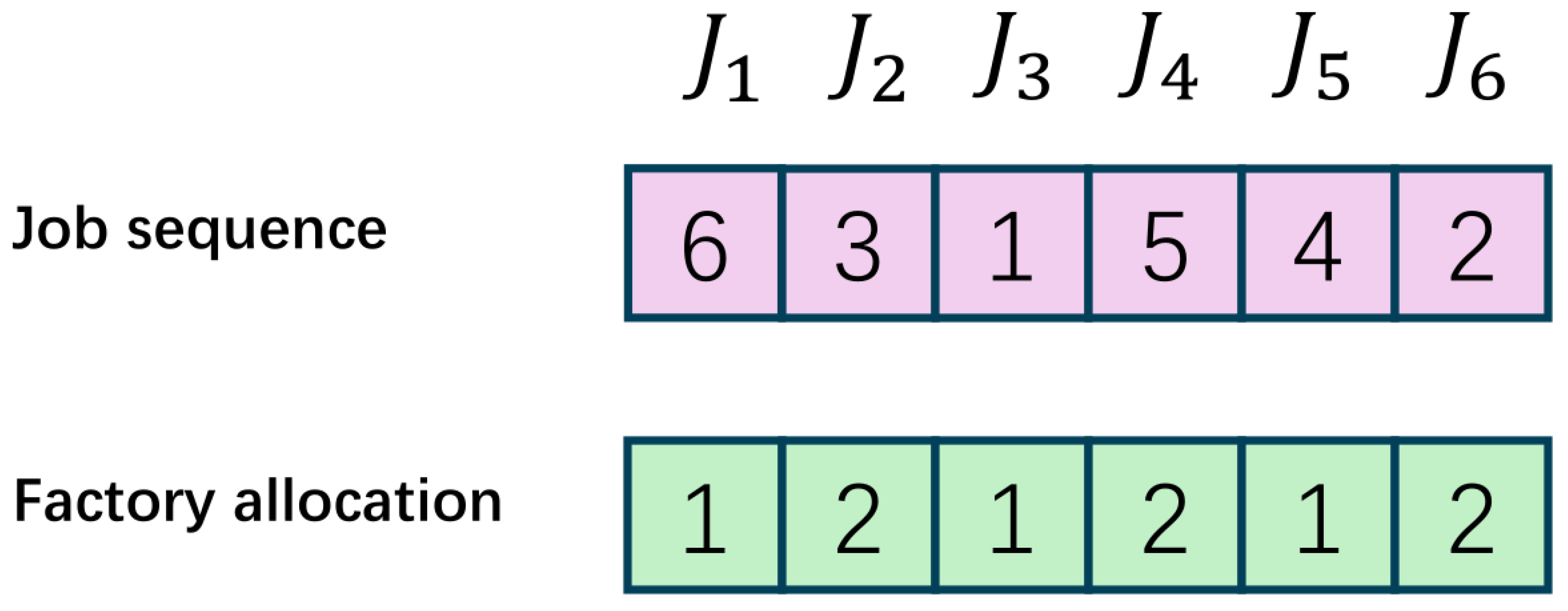
4.3. Encoding and Decoding

In this study, two one-dimensional vectors are used to convey a solution. $JS$ shows the processing sequence of different jobs. $FS$ shows the factory allocation of different jobs. Figure 2 shows a sample example of encoding schema. The number in the first line $(6,3,1,5,4,2)$ represents the job sequence of these six jobs, the second line implies the factory to which each job is assigned (assuming that there are two factories in total).

The decoding method converts the encoding values of $JS$ and $FS$ into appropriate scheduling schemes. Each job is allocated to the factory according to $FS$, and the job sequence of each factory is obtained by the job sequence. Then, jobs are assigned to each parallel machine under constraints.

Algorithm 1 The framework of the DRLBEA

1: Input: population size $\left(ps\right)$, learning rate $\left(lr\right)$, crossover rate $\left(P_c\right)$, mutation rate $\left(P_m\right)$. 2: Output: the Pareto solution set. 3: Initialization the population to generate $Pop$. (Section 4.5) 4: Generate the elite archive according to the fitness. 5: Train the neural network $\left(\theta \right)$ (Section 4.7) 6: while The stopping criterion is not satisfied do 7:     Perform selection, crossover, and mutation to generate a new population $\left(Po{p}_{new}\right)$, and calculate the fitness. 8:     Update the elite archive. 9:     An elite local search chooses the best action (the best local search strategy) via $\theta$ (Section 4.6) 10:    Energy saving strategy (Section 4.4). 11: end while 12: Write the elite in the Pareto solution set.

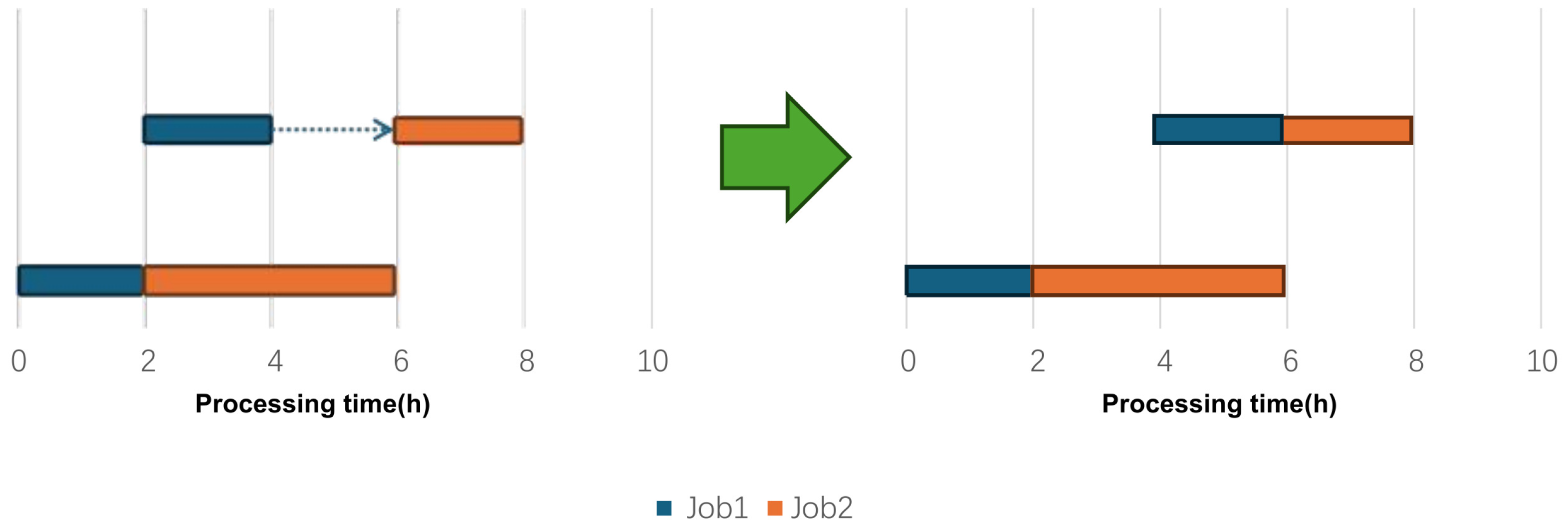
4.4. Energy-Saving Strategy

To achieve the goal of energy saving, one should consider idle power. This study adopts a right-shift strategy to achieve the purpose of reducing energy consumption. For a set of decoded solutions, the process of reverse decoding advances from the last job to the first job forward. First, determine whether it meets the conditions for rightward movement, that is, if (1) there is idle time behind the job, (2) the completion time of a job cannot exceed the deadline of that job, (3) the completion time of a job on a machine cannot exceed the start time of the next job, (4) the end time of that job cannot exceed the start time of the next phase; if these conditions are fulfilled, then rightward movement can be performed. The right-shift is performed within each phase and does not affect the completion time of the previous phase when the job is transferred to another phase. Then, the final impact results in a reduction in idle time, i.e., the energy consumption of the idle time machine is reduced, and the overall duration does not change. Assuming that there is idle time between two jobs at the same stage, in Figure 3, assuming that the idle power is 1 kW/h and the processing power is 3 kW/h, the due date of Job1 is 8, the due date of Job2 is 10, and a right-shift strategy can obviously be used; we know that the original $TEC=(2+4+2+2)\ast 3+2\ast 1=32$ kW, and after the right shift, $TEC=32-1\ast 2=30$ kW.

4.5. Initialization of DRLBEA

This section introduces the initialization of the DRLBEA. A high-quality initial solution is very important for solving the whole optimisation problem and can be the start of the whole solution process from a better solution set space. Many previous studies used multiple initialization methods to obtain a better initial solution [2,28]. In this study, several initialization methods were used:

(1) Problem features-based initialization, shown in Algorithm 2, where each job is sorted by priority in ascending order to generate a index array, and another sorting is based on the due date of each job in ascending order to generate another index array. The final array is the combination of two sets’ selection probabilities calculated through the algorithm in [23].

(2) Load balance initialization, where jobs are always assigned to the factory which has the minimum load.

(3) Random initialization, which randomly assigns a job sequence to each factory.

The original population was divided into equal-sized subpopulations; in this study, the numbers of subpopulations were $(3,4,5,10)$, The first and the second initialization had the same minimum subpopulation, and the remaining job sequences were generated randomly. Every time the initialization started, we selected one of them randomly as the result of the initialization.

Algorithm 2 Rank based on the priority and the due date

1: Input: population size $\left(ps\right)$, number of jobs $\left(N\right)$, due date of jobs $\left(D_i\right)$, priority of jobs $\left(R_i\right)$. 2: Output: processing sequence $JS$ 3: $R^{\prime }$: Ascending order of $R_i$ 4: $D^{\prime }$: Ascending order of $D_i$ 5: for Each $i\in [1,N]$ do 6:     $R_{R_i^{\prime }}=(N-i)/N$ 7:     $D_{D_i^{\prime }}=(N-i)/N$ 8:     $PRO=R_{R_i^{\prime }}+D_{D_i^{\prime }}$ 9: end for 10: $JS$: Ascending order of $PRO$

4.6. Global Search and Local Search

The proposed evolutionary algorithm is a hybrid framework. In this section, the global search and local search are introduced.

Global search: The population was first evolved through a global search. We chose a genetic algorithm [29] as the algorithmic framework, since genetic algorithms are applicable to various types of optimisation problems, do not depend on the specific mathematical form of the problem, and have strong adaptive ability to deal with more complex large-scale scheduling problems such as the DHGHFSP. Furthermore, genetic algorithms are simple to operate and easy to implement and extend. First, a tournament selection strategy [30] was applied to the individual selection. Then, we generated a new sequence via crossover. After that, mutation occurred to change some points in a sequence. Last, the outcome was combined with the population, the Pareto solutions were calculated by fast nondominated sorting and a crowding distance diversity strategy. The Algorithm 3 shows the whole course of events. All Pareto solutions were maintained within the elite archive.

Algorithm 3 Global search

1: Input: population size $\left(ps\right)$, rate of crossover $\left(P_c\right)$, rate of mutation $\left(P_m\right)$, number of jobs $\left(N\right)$, number of factories $\left(F\right)$, due date of jobs $\left(D_i\right)$, priority of jobs $\left(R_i\right)$, job sequence $\left(JS\right)$, factory allocation $\left(FS\right)$, elite archive $\left(ER\right)$. 2: Output: elite archive 3: Tournament selection to generate a new population $Po{p}_{new}$. 4: while  $i<Po{p}_{new}$  do 5:     Randomly generate a probability $\left(P_1\right)$. 6:     if $P_1<P_c$ then 7:          Precedence operation crossover [31] to generate a new job sequence $J{S}_1$. 8:          Uniform crossover [32] to generate new factory allocation $F{S}_1$. 9:     end if 10:    Randomly generate a probability $\left(P_2\right)$. 11:    if $P_2<P_m$ then 12:         Randomly swap two points to generate new job sequence $J{S}_2$. 13:         Randomly change a position to generate new factory allocation $F{S}_2$. 14:    end if 15: end while 16: Combine with $Po{p}_{new}$ and $ps$. 17: Nondominated sorting and crowding distance to obtain Pareto solutions. 18: Renew the elite archive $\left(E{R}^{\prime }\right)$.

Local search: There were four neighbourhood structures in this study. These four strategies focused on the critical job, that is, the job that had the biggest TWD.

(1) $L{S}_1$: Iterate backwards from the critical work; if the found job’s priority is smaller or the due date is earlier while the priority is the same, change these two jobs.

(2) $L{S}_2$: Iterate backwards from the critical work; if the found job’s priority is smaller or the due date is earlier while the priority is the same, insert the critical job before the found job.

(3) $L{S}_3$: Iterate backwards from the critical work; if the found job’s due date is smaller or the priority is earlier while the due date is the same, change these two jobs.

(4) $L{S}_4$: Iterate backwards from the critical work; if the found job’s due date is smaller or the priority is earlier while the due date is the same, insert the critical job before the found job.

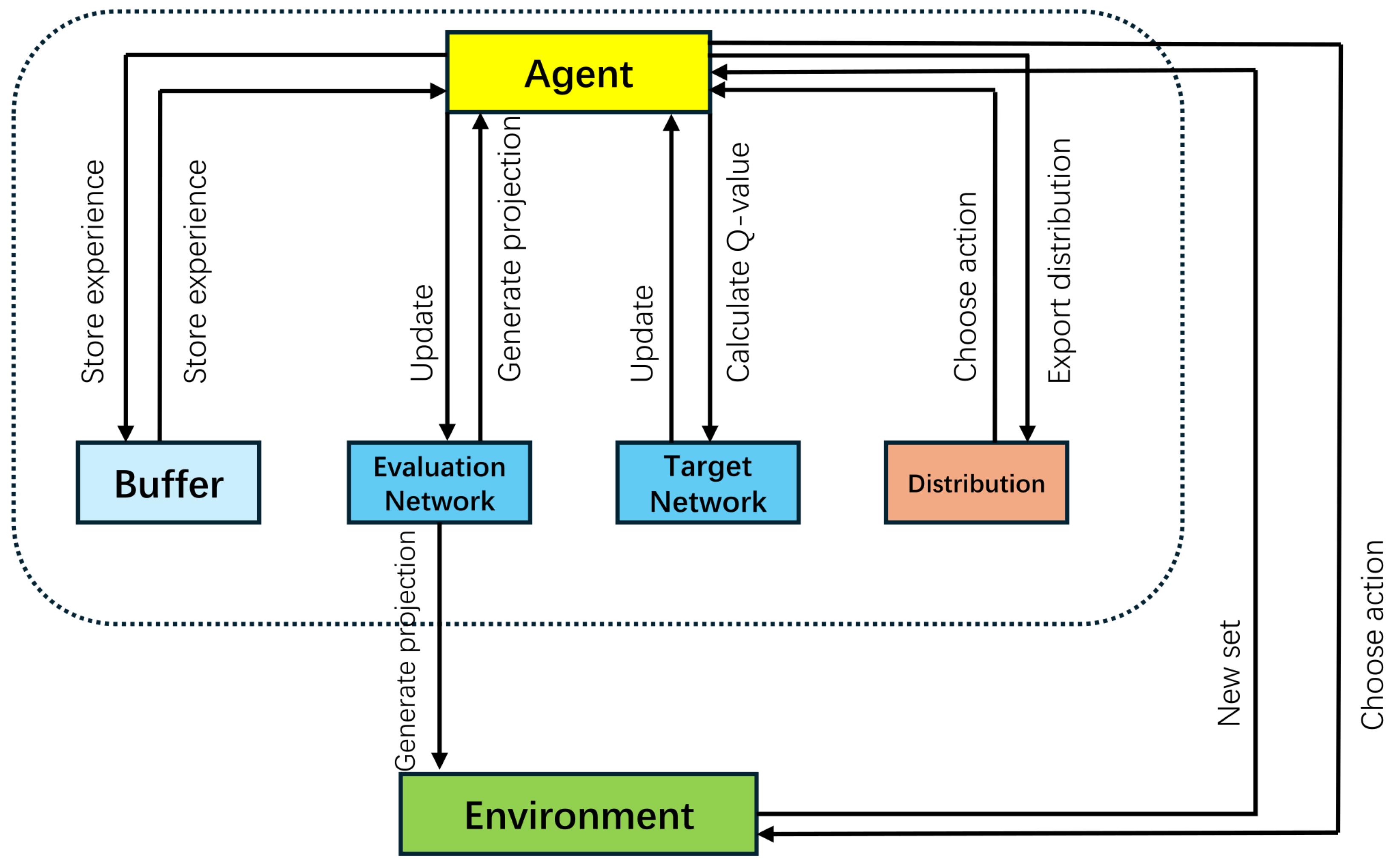
4.7. Distributional DQN for Operator Selection

In this section, a distributional DQN is trained for the operator selection of the local search; Figure 4 shows the structure. Two neural networks are utilized in the distributional DQN, an evaluation network (or online network) and a target network [33]. The distributional Q-function is a model of the distribution of Q-values. The evaluation network learns by interacting with the environment (Section 4.6, global search) directly and updating weights to estimate the Q-value distribution of the current state–action. The target network is used to calculate Q-values as follows:

$$\begin{array}{c}\hfill Q(s,a,z)=V(s,z)+A(s,a,z)-mean\left(A(s,a,z)\right)\end{array}$$

(15)

where $V(s,z)$ is the value distribution for the state s and atom z, and $A(s,a,z)$ is the advantage distribution for state s and action a at atom z. Compared to Q-learning, the distributional DQN has better learning performance and a more stable training process.

Neural network architecture: To facilitate feature extraction and generate value distributions, we designed a composite network comprising three layers: a feature layer, a value stream, and an advantage stream. Each part had two full connection layers and “ReLU” as the activation function. After that, softmax normalization was utilized to generate the action distribution.

Experience replay strategy: In order to improve the training efficiency and stability of the agent, the interactions between the agent and the environment needed to be stored to generate empirical data for subsequent updates. Pushing an experience included the state, action, reward, next state, and done flag $(S_t,A_t,R_t,S_{t+1},Don{e}_t)$ where $S_t$ is a vector formed by combining the JS and FA, and $A_t$ is the local search action in Section 4.6. The value of $R_t$ was given by the following definition: If the objectives $TWD$ and $TEC$ were smaller after executing the selected action, the reward was 20; if only $TWD$ was smaller, the reward was 15; if only $TEC$ is lower, the reward was 10; else the reward was 0. $Don{e}_t$ is a flag indicating whether the episode ends into the buffer. A new element was appended into the pool if the buffer was not full; otherwise, the earliest stored one was changed.

Training process: The agent chose an action according to the current state and epsilon-greedy policy [34]. Then, executing the corresponding action to obtain a set $(S_t,A_t,R_t,S_{t+1},Don{e}_t)$ to build a transition which was stored in the buffer. (1) For each sample in the batch, the agent computed the next state distribution (next state’s Q-atoms) using the target network. The target value $t_z$ for each atom was calculated by using the Bellman equation:

$$\begin{array}{c}\hfill t_z=r+(1-Done)·\gamma ·z^{\prime }\end{array}$$

(16)

where r is the reward received in the current state–action pair, $\gamma$ is a discount factor, which was set 0.9 in this study, $z^{\prime }$ is the next state value atom (bounded between $v_{min}=-10$ and $v_{max}=10$). (2) The target value $t_z$ was mapped to the closest atoms in the value distribution using linear interpolation. The indices of the nearest atoms were determined using the floor and ceil functions to approximate the target distribution over atoms. (3) The loss function used for training was the Categorical Cross-Entropy Loss between the predicted and target distributions over the value atoms. The predicted distribution was the one generated by the current policy (evaluation network), while the target distribution was derived from the target network; the loss function was as follows:

$$\begin{array}{c}\hfill Loss=-\sum _{·}(m_{i}log\left(p_i\right))\end{array}$$

(17)

where $m_i$ is the target probability mass for the ith atom, and $p_i$ is the predicted probability mass for the ith atom in the distribution. (4) The loss was minimized using backpropagation with the Adam optimiser. This updated the weights of the evaluation network to better approximate the true Q-distribution. At every iteration, the target network was updated with the weights of the evaluation network to ensure more stable training. The process is summarized in Algorithm 4.

Algorithm 4 Training process of Distributional DQN

1: Input: experience pool D, evaluation network ${\pi }_{\theta }\left(S\right)$, target network ${\pi }_{{\theta }^{\prime }}\left(S\right)$, support $\mathcal{Z}$, atom size K, batch size $bs$, learning rate $\alpha$, target update frequency T, maximum number of steps M. 2: Output: updated policy network ${\pi }_{\theta }\left(S\right)$, target network ${\pi }_{{\theta }^{\prime }}\left(S\right)$. 3: Initialize experience replay buffer D 4: Initialize evaluation network ${\pi }_{\theta }\left(S\right)$ with random weights 5: Initialize target network ${\pi }_{{\theta }^{\prime }}\left(S\right)$ with ${\pi }_{\theta }\left(S\right)$’s weights 6: Initialize optimiser for ${\pi }_{\theta }$ with learning rate $\alpha$ 7: $step=0$ 8: for  $step=1$  to  M  do 9:     if $step\%T=0$ then 10:          Update target network: ${\pi }_{{\theta }^{\prime }}\left(S\right)\leftarrow {\pi }_{\theta }\left(S\right)$ 11:    end if 12:    Sample a batch of transitions $\left\{(S_t,A_t,R_t,S_{t+1},Don{e}_t)\right\}$ from experience replay buffer D 13:    Compute the support (value atoms) for target distribution: 14:    $t_z=r_t+(1-Don{e}_t)·\gamma ·\mathcal{Z}$ 15:    Clip $t_z$ to the range $[v_{\min },v_{\max }]$ 16:    Compute the discrete target probability distribution m using interpolation: 17:    $m\left[l_i\right]+=\mathrm{next}\_\mathrm{dist}\left[i\right]·(u_i-b_i)$ 18:    $m\left[u_i\right]+=\mathrm{next}\_\mathrm{dist}\left[i\right]·(b_i-l_i)$ 19:    Compute the predicted probability distribution $q_{\theta }\left(S_t\right)$ from the evaluation network 20:    Compute the loss function: $Loss=-{\sum }_{i=1}^K{m}_i·log{q}_{\theta }(A_t,S_t,z_i)$ 21:    Update the evaluation network: $\theta \leftarrow \theta -\alpha ·{\nabla }_{\theta }L$ 22: end for

5. Experimental Results and Discussion

The proposed DRLBEA was implemented using pycharm with python 3.10 and cuda 12.3 on Win 11 and run on an AMD core Ryzen7 6500H 3.2 GHz processor and 16.0 GB of RAM and NVIDIA GeForce RTX 3060 GPU. There are few existing DHGHFSP benchmarks, so we used the instances proposed by Li et al. [35]. In the 20 instances, n = 20, 40, 60, 80, 100, $n_s$ = 3, 5, and f = 2, 3. In terms of energy consumption, the processing energy consumption was $E_{pro}=4.0$ kW/h, and the idle energy consumption was $E_{idle}$ = 1.0 kW/h. The instances were named aJbScF, where a, b, and c represent the total number of jobs, stages in each factory, and factories.

5.1. Evaluation Metrics

The hypervolume (HV) and Inverted Generational Distance (IGD) were used to represent the performance of the proposed DRLBEA. Before calculating the HV and IGD, solutions in nondominated should be normalized as follows:

$$\begin{array}{c}\hfill x_i^{\mathrm{norm}}={\displaystyle \frac{x_i-z_i^{min}}{z_i^{max}-z_i^{min}}},i=1,2\end{array}$$

(18)

where $z_i^{min}$ and $z_i^{max}$ is the minimum and maximum of the ith objective in the Pareto front.

(1)

HV metric:

$$\begin{array}{c}\hfill HV=V(\bigcup _{i=1}^P{V}_i)\end{array}$$

(19)

The HV is the volume of the region in the target space enclosed by the set of nondominated solutions and the reference point. P is the nondominated solution set, and $V_i$ is the hypercube formed between P and the reference point (the maximum value). In this study, we normalized the solution set; thus, the reference point was 1, 1. A higher HV has better algorithm synthesis performance.

(2)

IGD metric:

$$\begin{array}{c}\hfill IGD(P,P^{\ast })={\displaystyle \frac{1}{|P^{\ast }|}}\sum _{z\in P^{\ast }}\underset{x\in P}{min}d(z,x)\end{array}$$

(20)

The IGD measures the average distance from the points in the reference Pareto front to the generated solution set. P is the obtained nondominated solution set, $P^{\ast }$ is the Pareto front set, and $d(z,x)$ refers to the Euclidean distance between the reference point z and the point x in the solution set. A lower IGD means a better solution set.

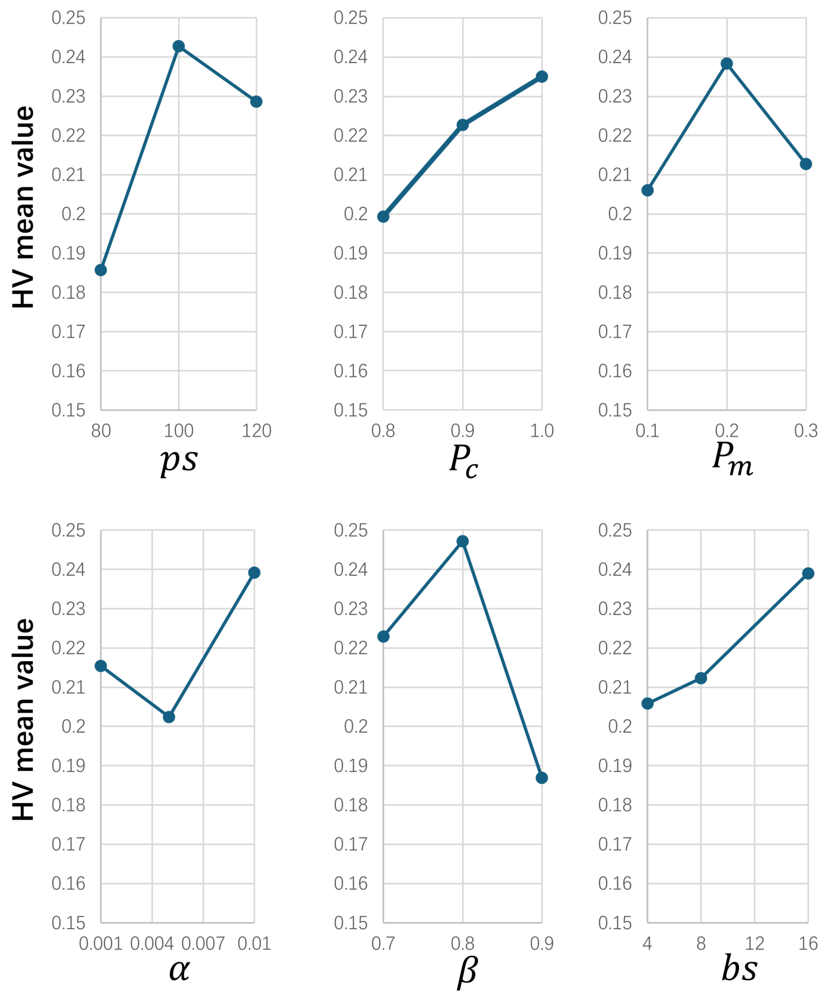
5.2. Parameter Setting

Different parameters affect the performance of the DRLBEA. In this study, six key parameters needed to be adjusted: the population size $ps=\{80,100,120\}$, the crossover rate $P_c=\{0.8,0.9,1.0\}$, the mutation rate $P_m=\{0.1,0.2,0.3\}$, the learning rate $\alpha =\{0.001,0.005,0.01\}$, the greedy factor $\beta =\{0.7,0.8,0.9\}$, the the batch size $bs=\{4,8,16\}$, and a design-of-experiment (DOE) Taguchi method [36] was applied to make sure the parameters were properly sampled. An orthogonal array $L_{18}\left(3^6\right)$ was used for the experiments, and we ran these 18 combinations ten times on a randomly generated pattern.

Table 4. Levels of parameters.

Trial	Level						HV
	ps	${\mathit{P}}_{\mathit{c}}$	${\mathit{P}}_{\mathit{m}}$	$\mathit{\alpha }$	$\mathit{\beta }$	$\mathit{b}\mathit{s}$
1	1	1	1	1	1	1	0.1835
2	1	2	2	2	2	2	0.2603
3	1	3	3	3	3	3	0.1661
4	2	1	2	2	3	1	0.1873
5	2	2	3	3	1	2	0.2463
6	2	3	1	1	2	3	0.2855
7	3	1	3	1	2	1	0.2121
8	3	2	1	2	3	2	0.1566
9	3	3	2	3	1	3	0.2974
10	1	1	3	3	2	1	0.1826
11	1	2	1	1	3	2	0.1508
12	1	3	2	2	1	3	0.1711
13	2	1	1	2	1	2	0.2081
14	2	2	2	3	2	3	0.2913
15	2	3	3	1	3	1	0.2381
16	3	1	2	1	3	3	0.2223
17	3	2	3	2	1	1	0.2311
18	3	3	1	3	2	2	0.2516

shows the mean HV of each parameter combination.

Figure 5 shows the result of the parameter setting experiments; the average HV was calculated six times. From the result, the best parameter configuration was $ps=100$, $P_c=1.0$, $P_m=0.2$, $\alpha =0.01$, $\beta =0.8$, and $bs=16$.

5.3. Evaluation of Each Strategy of DRLBEA

In this section, we used different conditions to verify the efficiency of each strategy. According to different improvements, we designed three experiments named $E{X}_i$, $i\in \{1,2,3,4\}$, to prove the effectiveness of the proposed DRLBEA.

Table 5. Derived HV mean value of DRLBEA and its variants across all instances.

Instances	HV
	${\mathit{E}\mathit{X}}_{\mathbf{1}}$	${\mathit{E}\mathit{X}}_{\mathbf{2}}$	${\mathit{E}\mathit{X}}_{\mathbf{3}}$	${\mathit{E}\mathit{X}}_{\mathbf{4}}$	DRLBEA
20J3S2F	0.7862	0.7970	0.8171	0.7865	0.8231
20J3S3F	0.6689	0.6637	0.6741	0.6159	0.6893
20J5S2F	0.7514	0.6690	0.7474	0.7656	0.7430
20J5S3F	0.7459	0.7208	0.7608	0.7808	0.8104
40J3S2F	0.7649	0.7509	0.7741	0.7747	0.8201
40J3S3F	0.7208	0.7171	0.7248	0.6949	0.8004
40J5S2F	0.6574	0.6603	0.6810	0.7036	0.7923
40J5S3F	0.7270	0.7200	0.7100	0.7095	0.8348
60J3S2F	0.6848	0.7324	0.6877	0.6210	0.7409
60J3S3F	0.6938	0.6458	0.7083	0.6402	0.7315
60J5S2F	0.7146	0.6936	0.6992	0.6382	0.7630
60J5S3F	0.6836	0.6852	0.6940	0.7398	0.6929
80J3S2F	0.6373	0.6604	0.6742	0.5783	0.7354
80J3S3F	0.8105	0.7776	0.8166	0.8455	0.8968
80J5S2F	0.7362	0.7529	0.7522	0.7813	0.7852
80J5S3F	0.6686	0.6760	0.6755	0.7515	0.6630
100J3S2F	0.4982	0.6278	0.5097	0.6725	0.7109
100J3S3F	0.7674	0.7885	0.7791	0.7632	0.8424
100J5S2F	0.6644	0.6989	0.6823	0.5229	0.7899
100J5S3F	0.6597	0.6278	0.6641	0.6075	0.6329

Bold values indicate the best HV performance for each instance.

shows the HV and

Table 6. Derived IGD mean value of DRLBEA and its variants across all instances.

Instances	IGD
	${\mathit{E}\mathit{X}}_{\mathbf{1}}$	${\mathit{E}\mathit{X}}_{\mathbf{2}}$	${\mathit{E}\mathit{X}}_{\mathbf{3}}$	${\mathit{E}\mathit{X}}_{\mathbf{4}}$	DRLBEA
20J3S2F	0.0328	0.0289	0.0244	0.0434	0.0225
20J3S3F	0.0136	0.0094	0.0121	0.0103	0.0120
20J5S2F	0.0406	0.0581	0.0304	0.0334	0.0294
20J5S3F	0.0191	0.0200	0.0247	0.0099	0.0168
40J3S2F	0.0510	0.0554	0.0495	0.0508	0.0418
40J3S3F	0.0385	0.0507	0.0562	0.0585	0.0335
40J5S2F	0.0839	0.0734	0.0956	0.0828	0.0689
40J5S3F	0.0568	0.0805	0.0839	0.0908	0.0701
60J3S2F	0.0366	0.0363	0.0411	0.0424	0.0280
60J3S3F	0.0414	0.0440	0.0516	0.0634	0.0348
60J5S2F	0.0667	0.0613	0.0773	0.0817	0.0536
60J5S3F	0.0585	0.0679	0.0533	0.0519	0.0459
80J3S2F	0.0691	0.0685	0.0624	0.0841	0.0527
80J3S3F	0.0838	0.1405	0.1015	0.0779	0.0549
80J5S2F	0.0991	0.1060	0.1411	0.1058	0.0657
80J5S3F	0.0984	0.0996	0.0887	0.0816	0.0863
100J3S2F	0.0832	0.0793	0.1052	0.0522	0.0338
100J3S3F	0.0567	0.1108	0.0702	0.0824	0.0879
100J5S2F	0.0821	0.0981	0.0973	0.1022	0.0631
100J5S3F	0.0787	0.0884	0.0912	0.1085	0.0634

Bold values indicate the best IGD performance for each instance.

shows the IGD obtained by these five algorithms over 20 instances. First, $E{X}_1$ represented the DRLBEA without the initialization strategy, where all individuals were randomly generated. The HV of $E{X}_1$ was higher than that of the DRLBEA on 3 instances and lower in the other 17 instances. As for IGD, DRLBEA had lower values than $E{X}_1$ on 18 instances; this indicated that our initialization strategy was efficient.

$E{X}_2$ represented the DRLBEA without deep reinforcement learning, where the local search strategy (Section 4.5) was randomly selected from four strategies to generate the new elite archive. The HV of DRLBEA was higher than that of $E{X}_2$ except for “80J5S3F”, the IGD of DRLBEA was lower than that of $E{X}_2$ except for “20J3S3F”. This means the deep reinforcement learning plays a vital role in the DRLBEA.

$E{X}_3$ represented the DRLBEA without the local search; the HV of $E{X}_3$ performed better than that of DRLBEA on 3 instances and worse than DRLBEA on 17 instances. The IGD of DRLBEA was lower than that of $E{X}_3$ on all instances. This result indicates that the local search strategy expands the search space and improve the performance of the DRLBEA.

$E{X}_4$ represented the DRLBEA without the energy-saving strategy, where we removed right-shift strategy from the DRLBEA to verify its efficiency. DRLBEA performed better than $E{X}_4$ on 16 instances; in other 4 instances, $E{X}_4$ performed slightly better than DRLBEA. These results show that the energy-saving strategy is efficient in reducing the energy consumption.

Table 7. Statistical value and Friedman’s test of all variant algorithms (significant level = 0.05).

Algorithms	HV			IGD
	Mean	Rank	p-Value	Mean	Rank	p-Value
$E{X}_1$	0.7021	3.70	4.4191 × 10−5	0.0595	3.05	2.0633 × 10−5
$E{X}_2$	0.7033	3.55		0.0689	3.50
$E{X}_3$	0.7116	2.75		0.0679	3.55
$E{X}_4$	0.6997	3.45		0.0657	3.50
DRLBEA	0.7649	1.55		0.0483	1.40

Bold values indicate the best statistical value performance.

shows the results of the Friedman’s rank-sum test, with a confidence level of $\alpha$ = 0.05. From the experimental results, we can conclude that a p-value of less than 0.05 demonstrates that the DRLBEA outperforms all variants, and the effectiveness of all strategies used in the DRLBEA.

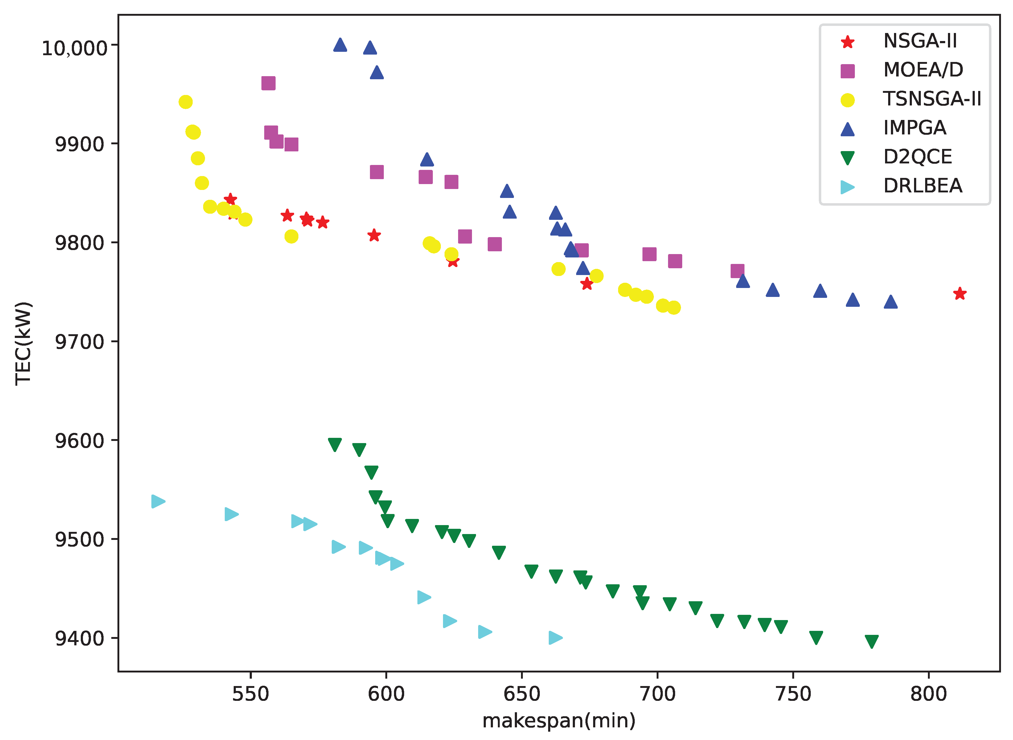
5.4. Comparison with Other Algorithms

Next, we compared the proposed DRLBEA with the state-of-the-art algorithms, including NSGA-II [37], MOEA/D [38], two-stage NSGA-II(TSNSGA-II) [39], IMPGA [24], D2QCE [35]. To further test the performance, all tested algorithms used the same encoding and decoding methods including the energy-saving strategy and ran on these 20 instances 20 times using the same stopping criterion. These algorithms adopted the same initialization and local search strategy. The parameter setting of each algorithm was as follows: (1) $ps$ was 100, $P_c$ was 1.0, $P_m$ was 0.8; (2) the neighbourhood size T was 10; (3) the inertial weight w, personal best weight $c_1$, global best weight $c_2$ of IMPGA were 0.5, 1.5, and 1.5, respectively; (4) for D2QCE, all parameters were set according to [36].

Table 8. Comparison of HV mean value on 20 instances.

Instances	HV
	NSGA-II	MOEA/D	TSNSGA-II	IMPGA	D2QCE	DRLBEA
20J3S2F	0.6866	0.6783	0.6684	0.1617	0.8261	0.9078
20J3S3F	0.7135	0.6463	0.7405	0.4143	0.6738	0.7056
20J5S2F	0.6969	0.7010	0.7454	0.3059	0.7678	0.8750
20J5S3F	0.7350	0.6771	0.7321	0.4468	0.7558	0.8328
40J3S2F	0.6740	0.5982	0.6624	0.4251	0.7425	0.8378
40J3S3F	0.6853	0.6619	0.7090	0.3005	0.7013	0.7914
40J5S2F	0.7008	0.7316	0.7431	0.5164	0.7231	0.8379
40J5S3F	0.6714	0.6871	0.6821	0.5812	0.7443	0.8572
60J3S2F	0.7214	0.7049	0.7458	0.5234	0.7030	0.7581
60J3S3F	0.6976	0.7037	0.7540	0.6577	0.7019	0.7925
60J5S2F	0.7609	0.7602	0.7282	0.5477	0.7135	0.8088
60J5S3F	0.6898	0.7180	0.7309	0.5109	0.6957	0.7508
80J3S2F	0.7754	0.6963	0.7894	0.5585	0.8073	0.7354
80J3S3F	0.7323	0.6285	0.7275	0.4277	0.7911	0.8987
80J5S2F	0.7438	0.6648	0.7658	0.4925	0.7500	0.8908
80J5S3F	0.6965	0.7060	0.6960	0.6745	0.7615	0.7623
100J3S2F	0.7730	0.7346	0.7378	0.4686	0.7249	0.7981
100J3S3F	0.7154	0.6775	0.7567	0.5471	0.7594	0.8693
100J5S2F	0.7752	0.6995	0.7848	0.2812	0.7853	0.8214
100J5S3F	0.7131	0.7131	0.6811	0.3651	0.7331	0.7849

Bold values indicate the best HV performance for each instance.

and

Table 9. Comparison of IGD mean value on 20 instances.

Instances	IGD
	NSGA-II	MOEA/D	TSNSGA-II	IMPGA	D2QCE	DRLBEA
20J3S2F	0.0939	0.0922	0.0540	0.4536	0.0346	0.0132
20J3S3F	0.1014	0.0693	0.0341	0.4324	0.0139	0.0077
20J5S2F	0.0945	0.0896	0.0197	0.2354	0.0458	0.0056
20J5S3F	0.0814	0.1034	0.0462	0.2131	0.0180	0.0068
40J3S2F	0.1128	0.1575	0.0840	0.2800	0.0715	0.0599
40J3S3F	0.1216	0.1780	0.1005	0.2875	0.0532	0.0464
40J5S2F	0.0938	0.1545	0.0914	0.1702	0.0704	0.0438
40J5S3F	0.1235	0.2123	0.0979	0.1349	0.0656	0.0404
60J3S2F	0.1045	0.1107	0.1018	0.2690	0.0360	0.0442
60J3S3F	0.1329	0.1018	0.1670	0.1995	0.0494	0.0274
60J5S2F	0.1101	0.1237	0.0823	0.1389	0.0626	0.0476
60J5S3F	0.1129	0.1593	0.1022	0.1593	0.0704	0.0582
80J3S2F	0.0811	0.1840	0.1144	0.1962	0.1236	0.0679
80J3S3F	0.1532	0.1580	0.1470	0.1783	0.0626	0.0622
80J5S2F	0.1145	0.2501	0.1304	0.1263	0.1217	0.0793
80J5S3F	0.1489	0.2219	0.1361	0.1275	0.0728	0.0539
100J3S2F	0.1339	0.1120	0.0955	0.1750	0.0744	0.0329
100J3S3F	0.1642	0.1638	0.1821	0.0939	0.0870	0.0429
100J5S2F	0.1381	0.2201	0.1450	0.3440	0.0864	0.0462
100J5S3F	0.1736	0.2145	0.2160	0.2539	0.0892	0.0557

Bold values indicate the best IGD performance for each instance.

show the results of all algorithms on each instance. Compared to other algorithms, the DRLBEA performed best for both HV and IGD metrics overall except in one instance of D2QCE, and IMPGA had the worst performance, which means we could achieve a better solution set when using the DRLBEA.

Moreover, Friedman’s test was performed to prove the superiority of the DRLBEA. We conducted 20 Friedman tests since all algorithms were run on each instance 20 times. The average statistical value, the average rank, and the average p-value are shown in

Table 10. Statistical value and Friedman’s test of all compared algorithms (significant level = 0.05).

Algorithms	HV			IGD
	Mean	Rank	p-Value	Mean	Rank	p-Value
NSGA-II	0.7179	3.60	1.0074 × 10−13	0.1195	4.00	1.3734 × 10−15
MOEA/D	0.6894	4.15		0.1538	4.75
TSNSGA-II	0.7291	3.10		0.1074	3.50
IMPGA	0.4603	6.00		0.2234	5.55
D2QCE	0.7431	2.90		0.0655	2.15
DRLBEA	0.8158	1.25		0.0422	1.05

Bold values indicate the best statistical value performance.

, the significant level was 0.05, where a p-value lower than 0.05 meant significant differences between the algorithms. DRLBEA performed better than other algorithms on most instances since the DRLBEA achieved the highest HV and IGD ranks.

Figure 6 is the visualization of different algorithms’ generated Pareto front on 20J2S3F. The figure shows that the DRLBEA was the closest to the coordinate origin, indicating a better solution set could be obtained through the DRLBEA.

5.5. Experiment on Real-World Case

To better assess the effectiveness of the DRLBEA, the compared algorithms were tested on a real-world case [35]. The algorithms in Section 5.4 were compared with the DRLBEA using the same settings.

Table 11. Statistical value and Friedman’s test of all compared algorithms (significant level = 0.05).

Algorithms	HV		IGD
	Mean	p-Value	Mean	p-Value
NSGA-II	0.7254	2.3241 × 10−9	0.0914	1.2150 × 10−9
MOEA/D	0.6896		0.1854
TSNSGA-II	0.6135		0.1635
IMPGA	0.4512		0.2154
D2QCE	0.7345		0.0854
DRLBEA	0.8606		0.0729

Bold values indicate the best statistical value performance.

shows the results; the DRLBEA clearly outperformed all compared algorithms in terms of HV and IGD metrics. The p-value < 0.05 implies that the DRLBEA performed better than the compared algorithms.

6. Conclusions

This article presented a deep reinforcement learning-based evolutionary algorithm to solve the distributed heterogeneous green hybrid flowshop scheduling problem. A multi-population initialization with hybrid initialization rules was used to improve the convergence and diversity. Then, an energy-saving strategy was devised to better reduce the energy consumption. Finally, a deep reinforcement learning-based local search selection was employed to achieve a better elite archive and obtain a more diversified solution set.

Many experiments designed to demonstrate the efficiency of the DRLBEA were conducted. We compared the DRLBEA with different combinations of improved strategies to verify the efficient of the DRLBEA. The DRLBEA was compared with other well-known algorithms on 20 instances of varying sizes, and it achieved better performance, obtaining a better Pareto front.

In the future, additional problems can be addressed, such as a more complex shop environment including dynamic events, the speed of machines, and heterogeneous parallel machines, using a wide application of deep reinforcement learning in scheduling problems.

References

1. Adel, A. Future of industry 5.0 in society: Human-centric solutions, challenges and prospective research areas. J. Cloud Comput.-Adv. Syst. Appl. 2022, 11, 40. [Google Scholar] [CrossRef] [PubMed]
2. Zhao, F.; He, X.; Wang, L. A Two-Stage Cooperative Evolutionary Algorithm with Problem-Specific Knowledge for Energy-Efficient Scheduling of No-Wait Flow-Shop Problem. IEEE Trans. Cybern. 2021, 51, 5291–5303. [Google Scholar] [CrossRef] [PubMed]
3. Li, J.Q.; Sang, H.Y.; Han, Y.Y.; Wang, C.G.; Gao, K.Z. Efficient multi-objective optimization algorithm for hybrid flow shop scheduling problems with setup energy consumptions. J. Clean. Prod. 2018, 181, 584–598. [Google Scholar] [CrossRef]
4. Neufeld, J.S.; Schulz, S.; Buscher, U. A systematic review of multi-objective hybrid flow shop scheduling. Eur. J. Oper. Res. 2023, 309, 1–23. [Google Scholar] [CrossRef]
5. Li, Y.Z.; Pan, Q.K.; Gao, K.Z.; Tasgetiren, M.F.; Zhang, B.; Li, J.Q. A green scheduling algorithm for the distributed flowshop problem. Appl. Soft Comput. 2021, 109. [Google Scholar] [CrossRef]
6. Ying, K.C.; Lin, S.W. Minimizing makespan for the distributed hybrid flowshop scheduling problem with multiprocessor tasks. Expert Syst. Appl. 2018, 92, 132–141. [Google Scholar] [CrossRef]
7. Chen, S.; Wang, X.; Wang, Y.; Gu, X. A knowledge-driven many-objective algorithm for energy-efficient distributed heterogeneous hybrid flowshop scheduling with lot-streaming. Swarm Evol. Comput. 2024, 91, 107526. [Google Scholar] [CrossRef]
8. Fernandes, J.M.R.C.; Homayouni, S.M.; Fontes, D.B.M.M. Energy-Efficient Scheduling in Job Shop Manufacturing Systems: A Literature Review. Sustainability 2022, 14, 6264. [Google Scholar] [CrossRef]
9. Lu, C.; Gao, L.; Yi, J.; Li, X. Energy-Efficient Scheduling of Distributed Flow Shop With Heterogeneous Factories: A Real-World Case From Automobile Industry in China. IEEE Trans. Ind. Inform. 2021, 17, 6687–6696. [Google Scholar] [CrossRef]
10. He, L.; Sun, S.; Luo, R. A hybrid two-stage flowshop scheduling problem. Asia-Pacific J. Oper. Res. 2007, 24, 45–56. [Google Scholar] [CrossRef]
11. Fan, J.; Li, Y.; Xie, J.; Zhang, C.; Shen, W.; Gao, L. A Hybrid Evolutionary Algorithm Using Two Solution Representations for Hybrid Flow-Shop Scheduling Problem. IEEE Trans. Cybern. 2023, 53, 1752–1764. [Google Scholar] [CrossRef] [PubMed]
12. Wang, Y.J.; Wang, G.G.; Tian, F.M.; Gong, D.W.; Pedrycz, W. Solving energy-efficient fuzzy hybrid flow-shop scheduling problem at a variable machine speed using an extended NSGA-II. Eng. Appl. Artif. Intell. 2023, 121, 105977. [Google Scholar] [CrossRef]
13. Chen, R.; Yang, B.; Li, S.; Wang, S. A self-learning genetic algorithm based on reinforcement learning for flexible job-shop scheduling problem. Comput. Ind. Eng. 2020, 149, 106778. [Google Scholar] [CrossRef]
14. Qiao, J.; He, M.; Sun, N.; Sun, P.; Fan, Y. Factors affecting the final solution of the bike-sharing rebalancing problem under heuristic algorithms. Comput. Oper. Res. 2023, 159, 106368. [Google Scholar] [CrossRef]
15. Ge, Z.; Wang, H. Integrated Optimization of Blocking Flowshop Scheduling and Preventive Maintenance Using a Q-Learning-Based Aquila Optimizer. Symmetry 2023, 15, 1600. [Google Scholar] [CrossRef]
16. Wang, J.J.; Wang, L. A Bi-Population Cooperative Memetic Algorithm for Distributed Hybrid Flow-Shop Scheduling. IEEE Trans. Emerg. Top. Comput. Intell. 2021, 5, 947–961. [Google Scholar] [CrossRef]
17. Zheng, J.; Wang, L.; Wang, J. A cooperative coevolution algorithm for multi-objective fuzzy distributed hybrid flow shop. Knowl.-Based Syst. 2020, 194, 105536. [Google Scholar] [CrossRef]
18. Zhang, G.; Liu, B.; Wang, L.; Yu, D.; Xing, K. Distributed Co-Evolutionary Memetic Algorithm for Distributed Hybrid Differentiation Flowshop Scheduling Problem. IEEE Trans. Evol. Comput. 2022, 26, 1043–1057. [Google Scholar] [CrossRef]
19. Zhang, G.; Ma, X.; Wang, L.; Xing, K. Elite Archive-Assisted Adaptive Memetic Algorithm for a Realistic Hybrid Differentiation Flowshop Scheduling Problem. IEEE Trans. Evol. Comput. 2022, 26, 100–114. [Google Scholar] [CrossRef]
20. Wang, J.J.; Wang, L. A Cooperative Memetic Algorithm with Learning-Based Agent for Energy-Aware Distributed Hybrid Flow-Shop Scheduling. IEEE Trans. Evol. Comput. 2022, 26, 461–475. [Google Scholar] [CrossRef]
21. Qin, H.X.; Han, Y.Y. A collaborative iterative greedy algorithm for the scheduling of distributed heterogeneous hybrid flow shop with blocking constraints. Expert Syst. Appl. 2022, 201, 117256. [Google Scholar] [CrossRef]
22. Shao, W.; Shao, Z.; Pi, D. An Ant Colony Optimization Behavior-Based MOEA/D for Distributed Heterogeneous Hybrid Flow Shop Scheduling Problem Under Nonidentical Time-of-Use Electricity Tariffs. IEEE Trans. Autom. Sci. Eng. 2022, 19, 3379–3394. [Google Scholar] [CrossRef]
23. Lin, C.C.; Peng, Y.C.; Chang, Y.S.; Chang, C.H. Reentrant hybrid flow shop scheduling with stockers in automated material handling systems using deep reinforcement learning. Comput. Ind. Eng. 2024, 189, 109995. [Google Scholar] [CrossRef]
24. Li, R.; Gong, W.; Wang, L.; Lu, C.; Dong, C. Co-Evolution With Deep Reinforcement Learning for Energy-Aware Distributed Heterogeneous Flexible Job Shop Scheduling. IEEE Trans. Syst. Man Cybern.-Syst. 2024, 54, 201–211. [Google Scholar] [CrossRef]
25. Vasquez, O.C. On the complexity of the single machine scheduling problem minimizing total weighted delay penalty. Oper. Res. Lett. 2014, 42, 343–347. [Google Scholar] [CrossRef]
26. Lim, B.; Vu, M. Distributed Multi-Agent Deep Q-Learning for Load Balancing User Association in Dense Networks. IEEE Wirel. Commun. Lett. 2023, 12, 1120–1124. [Google Scholar] [CrossRef]
27. Cui, H.; Li, X.; Gao, L. An improved multi-population genetic algorithm with a greedy job insertion inter-factory neighborhood structure for distributed heterogeneous hybrid flow shop scheduling problem. Expert Syst. Appl. 2023, 222, 119805. [Google Scholar] [CrossRef]
28. Yang, J.; Xu, H.; Cheng, J.; Li, R.; Gu, Y. A decomposition-based memetic algorithm to solve the biobjective green flexible job shop scheduling problem with interval type-2 fuzzy processing time. Comput. Ind. Eng. 2023, 183, 109513. [Google Scholar] [CrossRef]
29. Liu, S.C.; Chen, Z.G.; Zhan, Z.H.; Jeon, S.W.; Kwong, S.; Zhang, J. Many-Objective Job-Shop Scheduling: A Multiple Populations for Multiple Objectives-Based Genetic Algorithm Approach. IEEE Trans. Cybern. 2023, 53, 1460–1474. [Google Scholar] [CrossRef]
30. Yang, J.; Soh, C. Structural optimization by genetic algorithms with tournament selection. J. Comput. Civ. Eng. 1997, 11, 195–200. [Google Scholar] [CrossRef]
31. Zhang, C.; Li, P.; Rao, Y.; Li, S. A new hybrid GA/SA algorithm for the job shop scheduling problem. In Lecture Notes in Computer Science, Proceedings of the 5th European Conference on Evolutionary Computation in Combinatorial Optimization (EvoCOP 2005), Lausanne, Switzerland, 30 March–1 April 2005; Raidl, G., Gottlieb, J., Eds.; Springer: Berlin/Heidelberg, Germany, 2005; Volume 3448, pp. 246–259. [Google Scholar]
32. Yang, W.; Wang, B.; Quan, H.; Hu, C. Strategy uniform crossover adaptation evolution in a minority game. Chin. Phys. Lett. 2003, 20, 1659–1661. [Google Scholar]
33. Huang, L.; Fu, M.; Rao, A.; Irissappane, A.A.; Zhang, J.; Xu, C. A Distributional Perspective on Multiagent Cooperation with Deep Reinforcement Learning. IEEE Trans. Neural Networks Learn. Syst. 2024, 35, 4246–4259. [Google Scholar] [CrossRef] [PubMed]
34. Hao, J.; Yang, T.; Tang, H.; Bai, C.; Liu, J.; Meng, Z.; Liu, P.; Wang, Z. Exploration in Deep Reinforcement Learning: From Single-Agent to Multiagent Domain. IEEE Trans. Neural Networks Learn. Syst. 2024, 35, 8762–8782. [Google Scholar] [CrossRef]
35. Li, R.; Gong, W.; Wang, L.; Lu, C.; Pan, Z.; Zhuang, X. Double DQN-Based Coevolution for Green Distributed Heterogeneous Hybrid Flowshop Scheduling With Multiple Priorities of Jobs. IEEE Trans. Autom. Sci. Eng. 2024, 21, 6550–6562. [Google Scholar] [CrossRef]
36. Reynolds, P.S. Between two stools: Preclinical research, reproducibility, and statistical design of experiments. BMC Res. Notes 2022, 15, 73. [Google Scholar] [CrossRef] [PubMed]
37. Deb, K.; Pratap, A.; Agarwal, S.; Meyarivan, T. A fast and elitist multiobjective genetic algorithm: NSGA-II. IEEE Trans. Evol. Comput. 2002, 6, 182–197. [Google Scholar] [CrossRef]
38. Zhang, Q.; Li, H. MOEA/D: A multiobjective evolutionary algorithm based on decomposition. IEEE Trans. Evol. Comput. 2007, 11, 712–731. [Google Scholar] [CrossRef]
39. Ming, F.; Gong, W.; Wang, L. A Two-Stage Evolutionary Algorithm with Balanced Convergence and Diversity for Many-Objective Optimization. IEEE Trans. Syst. Man Cybern.-Syst. 2022, 52, 6222–6234. [Google Scholar] [CrossRef]
Figure 1. Gantt chat of example in Table 3.
Processes 13 00728 g001
Figure 2. Encoding representation.
Processes 13 00728 g002
Figure 3. Right-shift strategy.
Processes 13 00728 g003
Figure 4. The structure of the distributional DQN.
Processes 13 00728 g004
Figure 5. Parameter levels.
Processes 13 00728 g005
Figure 6. Pareto front of different algorithms on 20J3S2F.
Processes 13 00728 g006