Numerical Study of Suspension Viscosity Accounting for Particle–Fluid Interactions Under Low-Confinement Conditions in Two-Dimensional Parallel-Plate Flow

Abstract

Suspensions are prevalent in daily life and serve various purposes, including applications in food, medicine, and industry. Many of these suspensions display non-Newtonian characteristics stemming from particle–fluid interactions. Understanding the rheology of suspensions is critical for developing materials for applications across different fields. While Einstein’s viscosity formula is recognized as a key evaluation tool for suspension rheology, it does not apply when the solvent is a non-Newtonian fluid. Consequently, we explored how changes in the microstructure of suspensions influence their rheology, specifically focusing on changes in relative viscosity, through numerical simulations. The computational approaches used were the regularized lattice Boltzmann method and the virtual flux method. The computational model used was a two-dimensional parallel-plate channel, and the flow properties of the solvent were represented using the power-law model. Consequently, multiple particles migrated to two symmetrical points relative to the center, achieving mechanical equilibrium and moving closer to the center as the power-law index increased. Furthermore, the relative viscosity observed was lower than that predicted by Einstein’s viscosity formula, indicating that shear thinning could occur even with a power-law index above 1. Additionally, as the power-law index decreased, the relative viscosity also decreased.

1. Introduction

Suspensions are prevalent in daily life and serve various purposes in food, medicine, and industry. The rheology of suspensions exhibits complex properties influenced by several factors, including particle size, shape, the spatial arrangement of the dispersed particles, the fluid forces acting on the particles, the interactions between the particles and their container, and the interactions between the particles themselves [1,2,3]. As a result, many aspects remain unsolved. A thorough understanding of suspension rheology, particularly viscosity, is crucial, because it can be easily modified to meet various requirements [4]. According to Einstein’s viscosity formula [5], the effective viscosity ${\eta }_{\mathrm{eff}}$ of a suspension can be determined based on the concentration of suspended particles.

$${\eta }_{\mathrm{eff}}={\eta }_0\left(1+\left[\eta \right]\varphi \right).$$

(1)

where ${\eta }_0$ represents the viscosity of a particle-free fluid, $\left[\eta \right]$ denotes the intrinsic viscosity, and $\varphi$ signifies the area fraction in 2D systems. According to Einstein’s viscosity formula, intrinsic viscosity $\left[\eta \right]$ is well established as $\left[\eta \right]=2$ for 2D systems and $\left[\eta \right]=2.5$ for 3D systems [6]. Consequently, the viscosity can be determined based on the concentration. However, Einstein’s viscosity formula is only valid when particles are uniformly dispersed, small in size, present in low concentrations, and when the solvent is a Newtonian fluid. Therefore, Einstein’s viscosity equation is applicable when particles are isolated, but it cannot be applied when particle interactions or non-uniform particle dispersion occur or the solvent is non-Newtonian, and the behavior of relative viscosity under these conditions remains unclear.

It has been reported that changes in the microstructure of a suspension, defined by the relative positioning of dispersed particles, considerably influence its rheology [7,8]. One factor that can change this microstructure is the inertial migration of the particles. A notable example of this inertial migration is the Segré–Silberberg effect [9]. This phenomenon occurs in inertial flows in a channel, causing neutrally buoyant particles to concentrate at specific equilibrium positions in the radial direction. The equilibrium position occurs where the lift force, created by the velocity difference along the length of the particle, balances with the repulsive force from the channel wall [10]. Inamuro et al. showed that the equilibrium position resulting from the Segré–Silberberg effect shifted toward the center of the channel as the confinement increased [11]. Here, confinement refers to the ratio of the particle diameter to the channel width.

Furthermore, regarding the relationship between the suspension rheology and microstructure, it has been reported that the relative viscosity of suspensions containing a single particle remains the same when the vertical position of the particle and the level of confinement are equal [12]. It was found that as the particle approached the wall and the confinement increased, the relative viscosity increased. Building on this understanding, Okamura et al. explored the relationship between relative viscosity and the spatial arrangement of a single particle in two-dimensional parallel-plate flow. They proposed that the macroscopic viscosity of a low-concentration suspension can be estimated by summing the contributions to the relative viscosity resulting from the confinement and spatial arrangement of each particle [13]. Thus, the microstructure undergoes changes due to solvent effects and inertial migration, which in turn influence the rheology of the suspension. However, the abovementioned studies were performed on suspensions with a Newtonian solvent, and few numerical studies have focused on suspensions with a non-Newtonian solvent. In a previous study of suspensions with a non-Newtonian solvent, Hu et al. demonstrated that the equilibrium position owing to the Segré–Silberberg effect shifts toward the channel center for larger power-law indices in a solvent modeled as a power-law fluid [14]. Additionally, Tomioka and Fukui examined a suspension containing a single particle using the Herschel–Bulkley model to represent the non-Newtonian fluid of the solvent and explored how the non-Newtonian characteristics of the solvent affected the particle’s equilibrium position and relative viscosity [15].

In contrast, many aspects of particle behavior and relative viscosity that involve particle–particle interactions in suspensions with multiple particles and a non-Newtonian fluid as the solvent remain unresolved. Analyzing these interactions under low-confinement conditions is crucial because it enhances the computational stability by highlighting interfacial phenomena between particles [16] and the fluid while minimizing the impact of particle–particle interactions [17]. Consequently, this study investigates the flow characteristics of suspensions with multiple particles under low-confinement conditions using a non-Newtonian fluid as the solvent. Therefore, the focus of this research is to examine the flow properties of these suspensions under such conditions.

2. Method

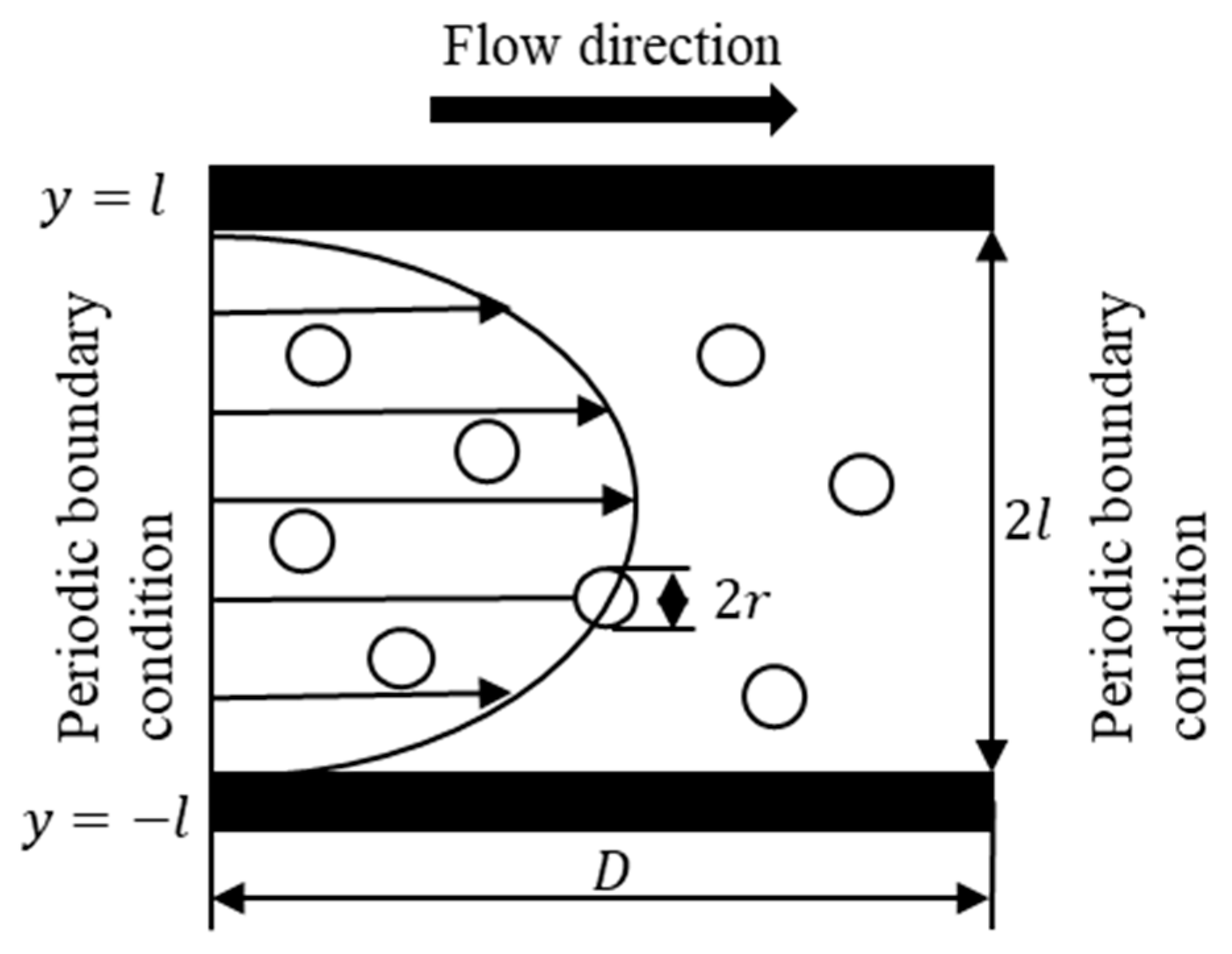
2.1. Computational Models

In this study, we analyzed the flow of particle suspensions between two-dimensional parallel-plates (Figure 1). We aimed to clarify the fundamental characteristics using circular particles. The rigid suspended particles were not treated as colloids, and since the particles were sufficiently large, Brownian motion was not taken into consideration. The particle interactions were considered via fluid dynamic forces. Additionally, the fluid was assumed to be in a steady state and incompressible. The particles were considered neutrally buoyant, and particle collisions were not confirmed during the simulation. The confinement was defined as the ratio of the particle diameter $2r$ to the channel width $2l$, with a value set at $C=2r/2l=0.025$, and the number of particles $N_{\mathrm{p}}$ was fixed at 16. Under these conditions, the concentration $\varphi$ corresponds to 0.79%. The channel length and characteristic length were defined as $D$, and the channel length $D$ was set equal to the channel width $2l$, and periodic boundary conditions, driven by pressure difference, were applied in the flow direction. To minimize the dependence on the initial particle positions, the analysis was based on the average results of 24 cases, each featuring randomly arranged particles.

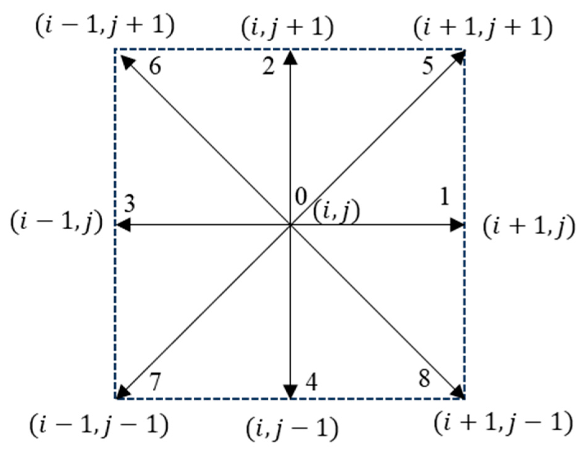
2.2. Governing Equation for Fluid

In this study, the regularized lattice Boltzmann method was used for the governing equation of the fluid [18]. This method retains the simplicity and efficiency of the original lattice Boltzmann approach while ensuring computational stability at high Reynolds numbers. Furthermore, it considerably decreases memory usage during the analysis. For this study, we adopted one of the most widely used models, the D2Q9 model. The division of this model is shown in Figure 2. In this model, the space is segmented into square lattices, where microscopic particles at a lattice point $\left(i,j\right)$ either remain at the same point $\left(i,j\right)$ or move in the direction indicated by the arrows shown in Figure 2 over one time step. The discrete velocities of the particles are defined by the following equation:

$${\mathit{e}}_{\alpha }=\left\{\begin{array}{cc}c\left(0,0\right)& \left(\alpha =0\right)\\ c\left(\cos {\displaystyle \frac{\left(\alpha -1\right)\pi }{2}},\sin {\displaystyle \frac{\left(\alpha -1\right)\pi }{2}}\right)& \left(\alpha =1–4\right).\\ \sqrt{2}c\left(\cos {\displaystyle \frac{\left(2\alpha -9\right)\pi }{2}},\sin {\displaystyle \frac{\left(2\alpha -9\right)\pi }{2}}\right)& \left(\alpha =5–8\right)\end{array} \right.$$

(2)

Here, $\alpha$ represents the tensor index and corresponds to the movement direction of virtual particles in the D2Q9 model, and $c$ represents the advection velocity, defined as $c=\delta x/\delta t$, where $\delta t$ is the time step and $\delta x$ is the spatial step. When the Boltzmann equation is discretized using the discrete velocity ${\mathit{e}}_{\alpha }$ and the collision relaxation time $\tau$, the following equation is derived:

$$f_{\alpha }\left(t+\delta t,\mathit{x}+{\mathit{e}}_{\alpha }\delta t\right)=f_{\alpha }\left(t,\mathit{x}\right)+{\displaystyle \frac{1}{\tau }}\left(f_{\alpha }^{\mathrm{eq}}\left(t,\mathit{x}\right)-f_{\alpha }\left(t,\mathit{x}\right)\right).$$

(3)

where $f_{\alpha }$ denotes the distribution function, while $f_{\alpha }^{\mathrm{eq}}$ represents the equilibrium distribution function. By applying the Chapman–Enskog expansion to the abovementioned equation, the Navier–Stokes equation can be derived. At this point, the relaxation time $\tau$ is defined by the following equation:

$$\tau ={\displaystyle \frac{3\nu }{c\delta \mathit{x}}}+{\displaystyle \frac{1}{2}}.$$

(4)

where $\nu$ represents the kinematic viscosity. The equilibrium distribution function is expressed as follows:

$$f_{\alpha }^{\mathrm{eq}}={\omega }_{\alpha }\rho \left\{1+{\displaystyle \frac{3\left({\mathit{e}}_{\alpha }·\mathit{u}\right)}{c^2}}+{\displaystyle \frac{9{\left({\mathit{e}}_{\alpha }·\mathit{u}\right)}^2}{2c^4}}-{\displaystyle \frac{3{\mathit{u}}^2}{2c^2}}\right\}.$$

(5)

Here, the weighting function in Equation (5) is defined as follows:

$${\omega }_{\alpha }=\left\{\begin{array}{cc}4/9& \left(\alpha =0\right)\\ 1/9& \left(\alpha =1–4\right) \\ 1/36& \left(\alpha =5–8\right)\end{array} \right.$$

(6)

Additionally, the density $\rho$, momentum $\rho \mathit{u}$, and stress tensor ${\Pi }_{ij}$, respectively, are given by the following equations:

$$\rho ={\displaystyle \sum }_{\alpha }{f}_{\alpha },$$

(7)

$$\rho \mathit{u}={\displaystyle \sum }_{\alpha }{\mathit{e}}_{\alpha }{f}_{\alpha },$$

(8)

$${\Pi }_{ij}\left(t,\mathit{x}\right)={\displaystyle \sum }_{\alpha }{e}_{\alpha i}{e}_{\alpha j}{\displaystyle \frac{p_{\alpha }\left(t,\mathit{x}\right)}{c_s^2}}.$$

(9)

Here, $c_s$ represents the speed of sound and is defined as follows:

$$c_s={\displaystyle \frac{1}{\sqrt{3}}}$$

(10)

The nonequilibrium part of the pressure distribution $p_{\alpha }^{\mathrm{neq}}$ and the nonequilibrium part of the stress tensor ${\Pi }_{ij}^{\mathrm{neq}}$ can be expressed as follows:

$$p_{\alpha }^{\mathrm{neq}}\left(t,\mathit{x}\right)=p_{\alpha }\left(t,\mathit{x}\right)-p_{\alpha }^{\mathrm{eq}}\left(t,\mathit{x}\right),$$

(11)

$${\Pi }_{ij}^{\mathrm{neq}}\left(t,\mathit{x}\right)={\Pi }_{ij}\left(t,\mathit{x}\right)-{\Pi }_{ij}^{\mathrm{eq}}\left(t,\mathit{x}\right).$$

(12)

By applying the Chapman–Enskog expansion, the nonequilibrium part of the pressure distribution function can be transformed as follows:

$$p_{\alpha }^{\mathrm{neq}}\left(t,\mathit{x}\right)\cong -\delta t\tau {\omega }_{\alpha }{Q}_{\alpha ij}{\mathsf{\partial }}_i\rho u_j.$$

(13)

where $Q_{\alpha ij}$ is the normalized tensor, defined as $Q_{\alpha ij}=e_{\alpha i}{e}_{\alpha j}-c_s^2{\mathsf{\partial }}_{ij}$. Furthermore, using Equations (9) and (12), the nonequilibrium part of the stress tensor can be expressed as follows:

$${\Pi }_{ij}^{\mathrm{neq}}\left(t,\mathit{x}\right)\cong -\delta t{c}_s^2\tau \left({\mathsf{\partial }}_i\rho u_j+{\mathsf{\partial }}_j\rho u_i\right).$$

(14)

From Equations (11) and (12), $p_{\alpha }^{\mathrm{neq}}$ can be expressed as follows:

$$p_{\alpha }^{\mathrm{neq}}\left(t,\mathit{x}\right)\cong {\displaystyle \frac{{\omega }_{\alpha }}{2c_s^2}}{Q}_{\alpha ij}{\Pi }_{ij}^{\mathrm{neq}}\left(t,\mathit{x}\right),$$

(15)

$$p_{\alpha }\left( t+\delta t , \mathit{x}+{\mathit{e}}_{\alpha }\delta t \right)=p_{\alpha }^{\mathrm{eq}}\left(t,\mathit{x}\right)+\left(1-{\displaystyle \frac{1}{\tau }}\right)p_{\alpha }^{\mathrm{neq}}\left(t,\mathit{x}\right).$$

(16)

2.3. Governing Equation for Suspended Particles

In this study, we adopted the two-way coupling scheme [19] to account for particle–fluid interactions. When a particle is subjected to fluid forces and moves, Newton’s second law governs its translational motion, while Euler’s equation of motion applies to its rotational motion. Consequently, these motions can be represented by the following equations:

$${\mathit{F}}_{\mathrm{p}}=m_{\mathrm{p}}{\displaystyle \frac{d^2{\mathit{x}}_{\mathrm{p}}}{d{t}^2}},$$

(17)

$$T_{\mathrm{p}}=I_{\mathrm{p}}{\displaystyle \frac{d^2{\theta }_{\mathrm{p}}}{d{t}^2}}.$$

(18)

where ${\mathit{F}}_{\mathrm{p}}$ denotes the force vector acting on the particle, $m_{\mathrm{p}}$ represents the particle mass, ${\mathit{x}}_{\mathrm{p}}$ is the particle’s position vector, $T_{\mathrm{p}}$ is the torque applied to the particle, $I_{\mathrm{p}}$ is the particle’s moment of inertia, and ${\theta }_{\mathrm{p}}$ is the particle’s rotation angle. Equations (17) and (18) are discretized using the third-order accurate Adams–Bashforth method.

$${\dot{\mathit{x}}}_{\mathrm{p}}^{n+1}={\dot{\mathit{x}}}_{\mathrm{p}}^n+\Delta t{\displaystyle \frac{23{\mathit{F}}_{\mathrm{p}}^n-16{\mathit{F}}_{\mathrm{p}}^{n-1}+5{\mathit{F}}_{\mathrm{p}}^{n-2}}{12m_{\mathrm{p}}}},$$

(19)

$${\mathit{x}}_{\mathrm{p}}^{n+1}={\mathit{x}}_{\mathrm{p}}^n+\Delta t{\displaystyle \frac{5{\mathit{u}}_{\mathrm{p}}^{n+1}+8{\mathit{u}}_{\mathrm{p}}^n-{\mathit{u}}_{\mathrm{p}}^{n-1}}{12}},$$

(20)

$${\dot{\theta }}_{\mathrm{p}}^{n+1}={\dot{\theta }}_{\mathrm{p}}^n+\Delta t{\displaystyle \frac{23T_{\mathrm{p}}^n-16T_{\mathrm{p}}^{n-1}+5T_{\mathrm{p}}^{n-2}}{12I_{\mathrm{p}}}},$$

(21)

$${\theta }_{\mathrm{p}}^{n+1}={\theta }_{\mathrm{p}}^n+\Delta t{\displaystyle \frac{5{\dot{\theta }}_{\mathrm{p}}^{n+1}+8{\dot{\theta }}_{\mathrm{p}}^n-{\dot{\theta }}_{\mathrm{p}}^{n-1}}{12}}.$$

(22)

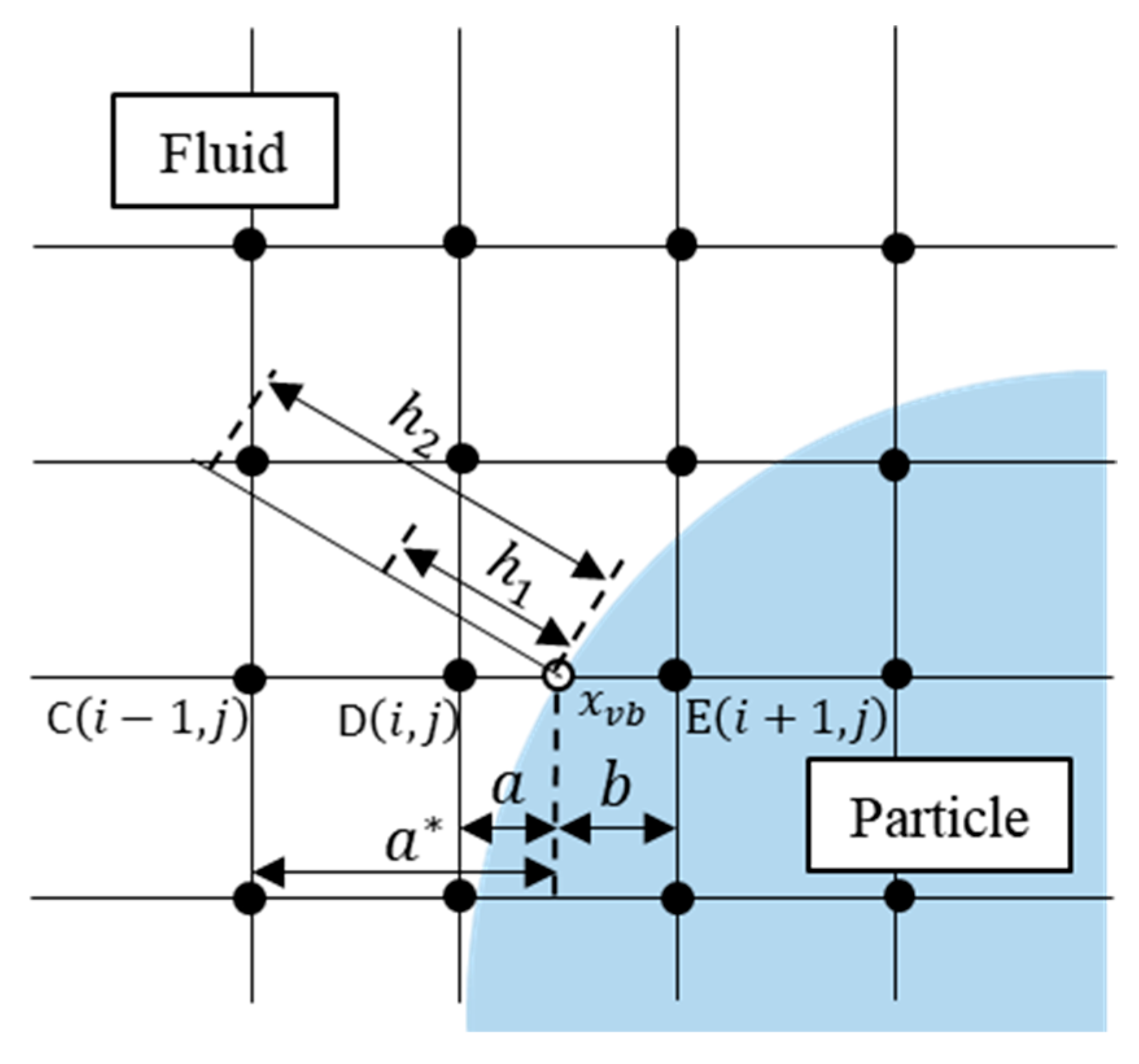
2.4. Virtual Flux Method

In this study, the virtual flux method [20,21] was used to represent circular rigid particles on a Cartesian grid. This method has several advantages. It effectively captures physical quantities around objects, is easy to implement, operates faster than the commonly used immersed boundary method (IBM), and allows for arbitrary selection of interpolation accuracy based on the distance between particles [22,23]. Figure 3 shows a schematic diagram of the virtual flux method.

In the virtual flux method, a virtual distribution function is used at points near the virtual boundary points. This virtual distribution function is required to satisfy the boundary conditions at the virtual boundary. The no-slip boundary condition is applied to the velocity, while a zero pressure gradient in the normal direction is used as an approximate boundary condition for pressure, as indicated in Equations (23) and (24):

$${\mathit{u}}_{\mathrm{vb}}={\mathit{u}}_{\mathrm{wall}},$$

(23)

$${\displaystyle \frac{\mathsf{\partial }p}{\mathsf{\partial }\mathit{n}}}=0.$$

(24)

The distribution function at the virtual boundary is expressed using the following equation:

$$f_{\alpha }\left(t,x_{\mathrm{vb}}\right)=f_{\alpha }^{\mathrm{eq}}\left(t,x_{\mathrm{vb}}\right)+\left\{f_{\alpha }\left(t,x_{\mathrm{D}}\right)-f_{\alpha }^{\mathrm{eq}}\left(t,x_{\mathrm{D}}\right)\right\}.$$

(25)

Referring to Figure 3, the equilibrium distribution function at the virtual boundary point $x_{\mathrm{vb}}$ can be obtained using the following equation:

$$f_{\alpha }^{\mathrm{eq}}\left(t,x_{\mathrm{vb}}\right)={\omega }_{\alpha }\rho \left[1+{\displaystyle \frac{3\left({\mathit{e}}_{\alpha }· {\mathit{u}}_{\mathrm{vb}}\right)}{c^2}}+{\displaystyle \frac{9{\left({\mathit{e}}_{\alpha }· {\mathit{u}}_{\mathrm{vb}}\right)}^2}{2c^4}}-{\displaystyle \frac{3{\mathit{u}}_{\mathrm{vb}}^2}{2c^2}}\right].$$

(26)

where ${\mathit{u}}_{\mathrm{vb}}$ denotes the velocity vector at the virtual boundary point, while $n$ represents the normal vector to the virtual boundary. Additionally, the virtual distribution function $f_{\alpha }^{*}\left(t,x_{\mathrm{E}}\right)$ and the virtual equilibrium distribution function $f_{\alpha }^{{\mathrm{eq}}^{*}}\left(t,x_{\mathrm{E}}\right)$ at point $\mathrm{E}$ are expressed via linear extrapolation using the internal division ratios $a$ and $b$, as given in the following equations:

$$f_{\alpha }^{*}\left(t,x_{\mathrm{E}}\right)={\displaystyle \frac{a+b}{a}}{f}_{\alpha }\left(t,x_{\mathrm{vb}}\right)-{\displaystyle \frac{b}{a}}{f}_{\alpha }\left(t,x_{\mathrm{D}}\right) ,$$

(27)

$$f_{\alpha }^{{\mathrm{eq}}^{*}}\left(t,x_{\mathrm{E}}\right)={\displaystyle \frac{a+b}{a}}{f}_{\alpha }^{\mathrm{eq}}\left(t,x_{\mathrm{vb}}\right)-{\displaystyle \frac{b}{a}}{f}_{\alpha }^{\mathrm{eq}}\left(t,x_{\mathrm{D}}\right)$$

(28)

Because we used an incompressible formulation, the equilibrium function $p_{\alpha }^{\mathrm{eq}}\left(t,x_{\mathrm{vb}}\right)$ at the object surface is as follows:

$$p_{\alpha }^{\mathrm{eq}}\left(t,x_{\mathrm{vb}}\right)={\omega }_{\alpha }\left[p_{\mathrm{vb}}+{\rho }_0\left\{\left({\mathit{e}}_{\alpha }· {\mathit{u}}_{\mathrm{vb}}\right)+{\displaystyle \frac{3{\left({\mathit{e}}_{\alpha }· {\mathit{u}}_{\mathrm{vb}}\right)}^2}{2c^2}}-{\displaystyle \frac{{\mathit{u}}_{\mathrm{vb}}^2}{2}}\right\}\right].$$

(29)

where $p_{\mathrm{vb}}$ represents the pressure at the virtual boundary. When the pressures $p_1$ and $p_2$ at points located at a distance $h_1$ and $h_2$ away from the boundary point in the normal direction to the wall are used, $p_{\mathrm{vb}}$ can be expressed using the following equation:

$$p_{\mathrm{vb}}={\displaystyle \frac{{h_2}^2{p}_1-{h_1}^2{p}_2}{{h_2}^2-{h_1}^2}}.$$

(30)

where $p_1$ and $p_2$ are calculated by interpolating the pressures at each of the four surrounding grid points. In this case, $h_1$ and $h_2$ were set to $\sqrt{2}$ and $2\sqrt{2}$ times the lattice size, respectively.

2.5. Power-Law Model

The non-Newtonian fluid properties of the solvent were modeled using the power-law model [24]. The strain rate tensor for a viscous fluid can be expressed in terms of the nonequilibrium component of the density distribution function $f_{\alpha }^{\mathrm{neq}}$, as follows:

$$S_{ij}={\displaystyle \frac{1}{2}}\left({\nabla }_j{u}_i+{\nabla }_i{u}_j\right)=-{\displaystyle \frac{3}{2\tau }}{\displaystyle \sum }_{\alpha }{f}_{\alpha }^{\mathrm{neq}}{e}_{\alpha i}{e}_{\alpha j}.$$

(31)

In this model, the apparent viscosity is given by the following:

$$v\left(\dot{\gamma }\right)=m{\left|\dot{\gamma }\right|}^{n-1}.$$

(32)

where $m$ represents the power-law constant, and $n$ signifies the power-law index. The power-law constant $m$ can be calculated using the following equation, which incorporates the Reynolds number $Re$, the representative velocity $U$, the representative length $D$, and the power-law index $n$:

$$Re={\displaystyle \frac{U^{2-n}{D}^n}{m}}.$$

(33)

The shear rate $\dot{\gamma }$ and the second invariant of the strain rate tensor $D_{\mathit{II}}$ are given by the following:

$$\dot{\gamma }= 2\sqrt{D_{\mathit{II}}},$$

(34)

$$D_{\mathit{II}}={\displaystyle \sum }_{i,j}^2{S}_{ij}{S}_{ij}.$$

(35)

2.6. Evaluation Method of Relative Viscosity

In this study, relative viscosity was used to assess the flow characteristics. The area flow rate $Q_0$ in a Poiseuille flow in a 2D parallel-plate channel without particles is described by the distance $l$ from the channel center to the wall, the viscosity ${\eta }_0$ of the particle-free fluid, and the pressure difference $\Delta p_0$ per unit of channel length $D$.

$$Q_0={\displaystyle \frac{2l^3}{3{\eta }_0}}{\displaystyle \frac{\Delta p_0}{D}}.$$

(36)

Similarly, the area flow rate $Q$ in a Poiseuille flow with particles is assumed to be determined using the effective viscosity ${\eta }_{\mathrm{eff}}$ of the suspension and the pressure difference $\Delta p$ [13]:

$$Q={\displaystyle \frac{2l^3}{3{\eta }_{\mathrm{eff}}}}{\displaystyle \frac{\Delta p}{D}}.$$

(37)

Therefore, the relative viscosity $\eta$ can be evaluated using the following equation, when $Q_0=Q$:

$$\eta ={\displaystyle \frac{{\eta }_{\mathrm{eff}}}{{\eta }_0}}={\displaystyle \frac{\Delta p}{\Delta p_0}}.$$

(38)

2.7. Simulation Codes

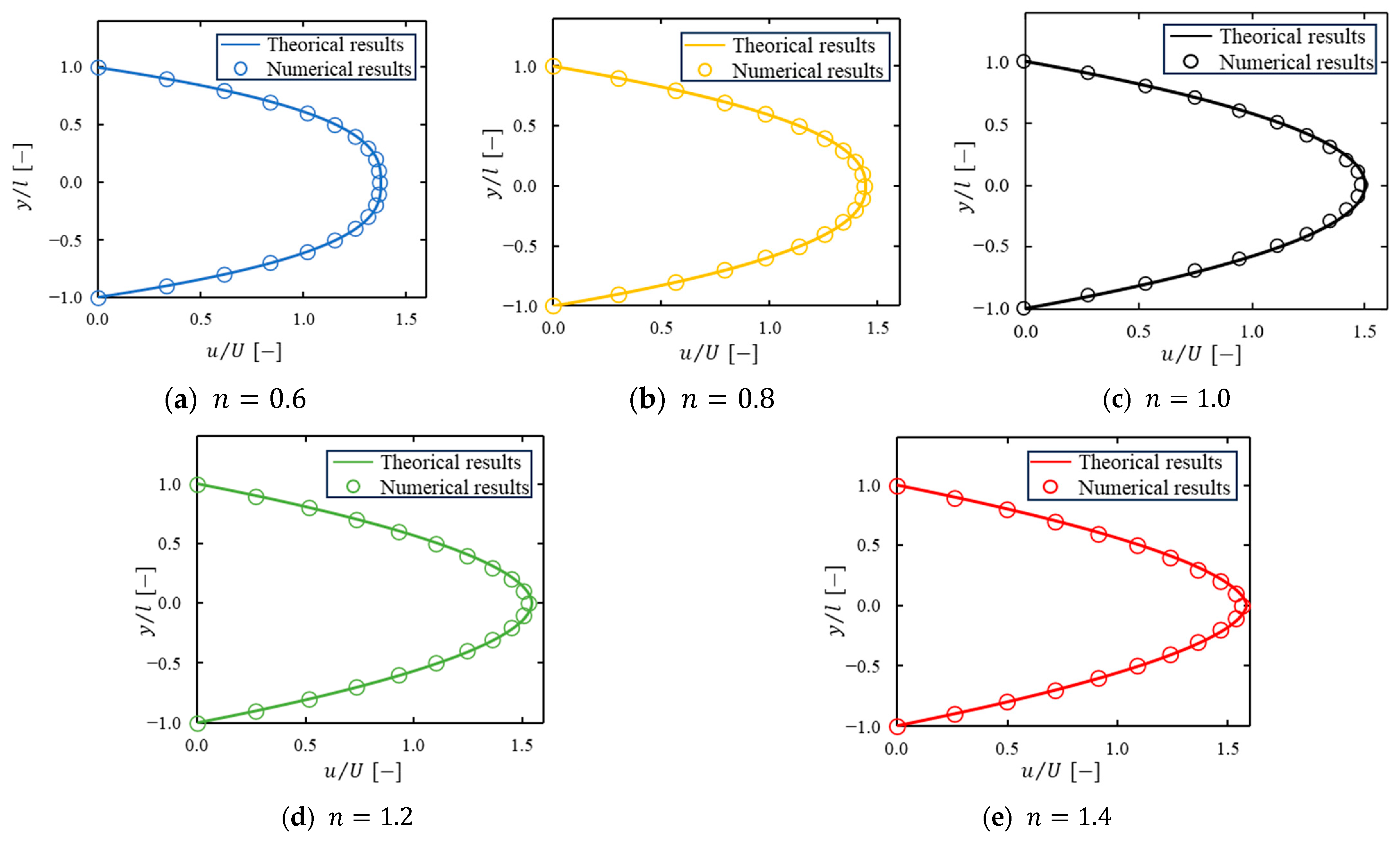
All simulation codes were homemade using Fortran 90/95. Additionally, Intel Fortran Compiler was used for their compilation.

3. Validation

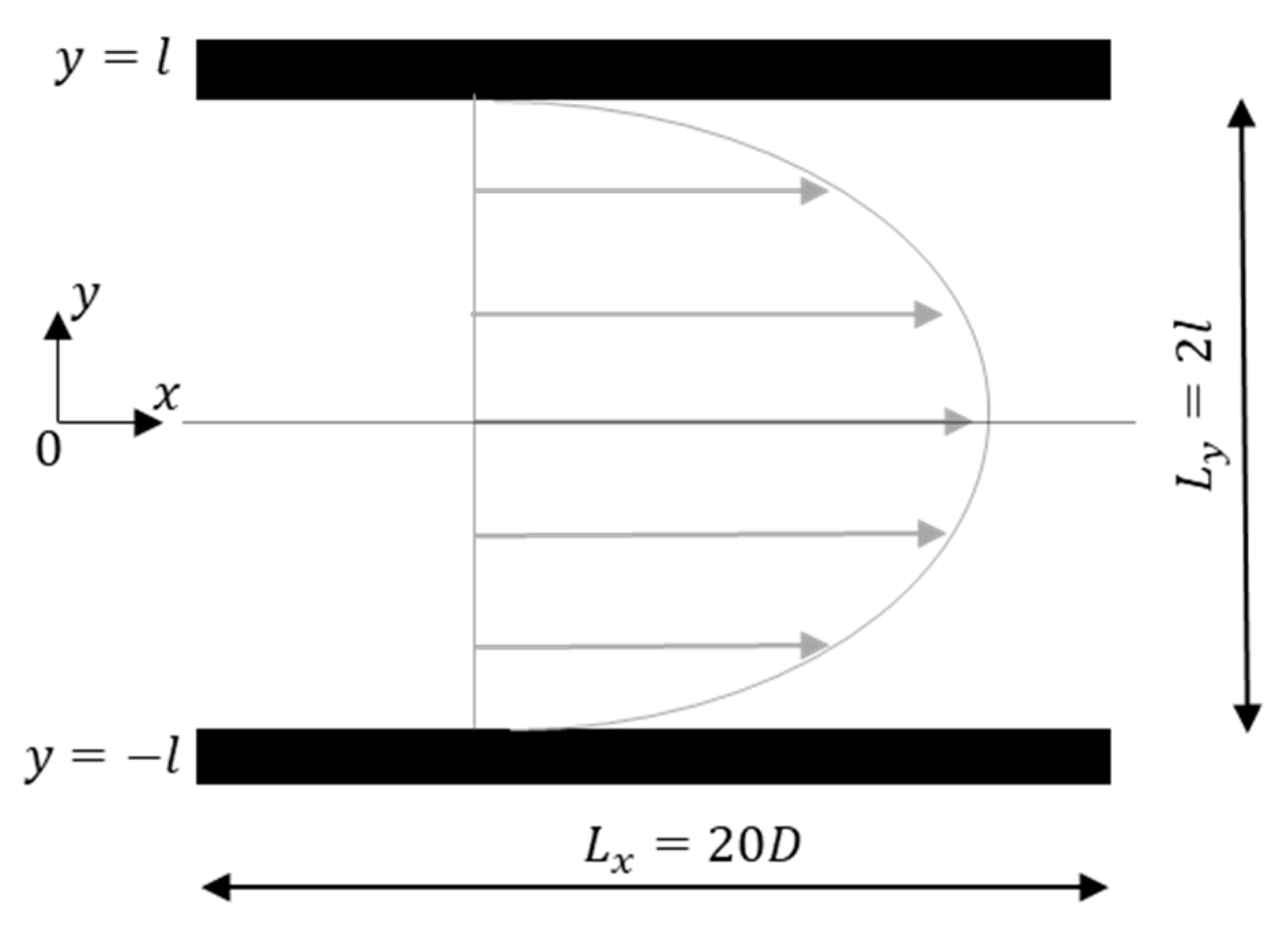
3.1. Simulation Models

The computational model is shown in Figure 4. Five different power-law indices for the solvent phase were used: (a) $n=0.6$, (b) $n=0.8$, (c) $n=1.0$, (d) $n=1.2$, and (e) $n=1.4$.

3.2. Results

Figure 5 shows the velocity distribution at $x/D=15$ when the power-law index is varied in the two-dimensional parallel-plate flow. The $\pm 1$ on the horizontal axis represents the channel walls, and 0 represents the channel center along the $y$-direction. The theoretical velocity of the power-law fluid in the two-dimensional channel is expressed by the following equation:

$$u\left(y\right)={\displaystyle \frac{2n+1}{n+1}}U\left[1-{\left|{\displaystyle \frac{y}{l}}\right|}^{{\displaystyle \frac{n+1}{n}}}\right]$$

(39)

The errors between the analytical results and theoretical values are shown in

Table 1. Mean squared error compared to theoretical values of non-Newtonian fluids for different power-law indices.

$n$	$0.6$	$0.8$	$1.0$	$1.2$	$1.4$
Error [%]	$0.60$	$0.66$	$0.79$	$0.99$	$1.22$

. The error increases with the power-law index. This is because as the power-law index increases, the rate of change in the velocity near the channel center becomes larger, and the number of lattice points used in the analysis is insufficient. Additionally, for all power-law indices, the error between the analytical results and theoretical values is less than 1.5%. Furthermore, since the velocity near the channel center increases and becomes sharper at the peak as the power-law index increases, the physical validity of the results is also confirmed.

4. Results and Discussion

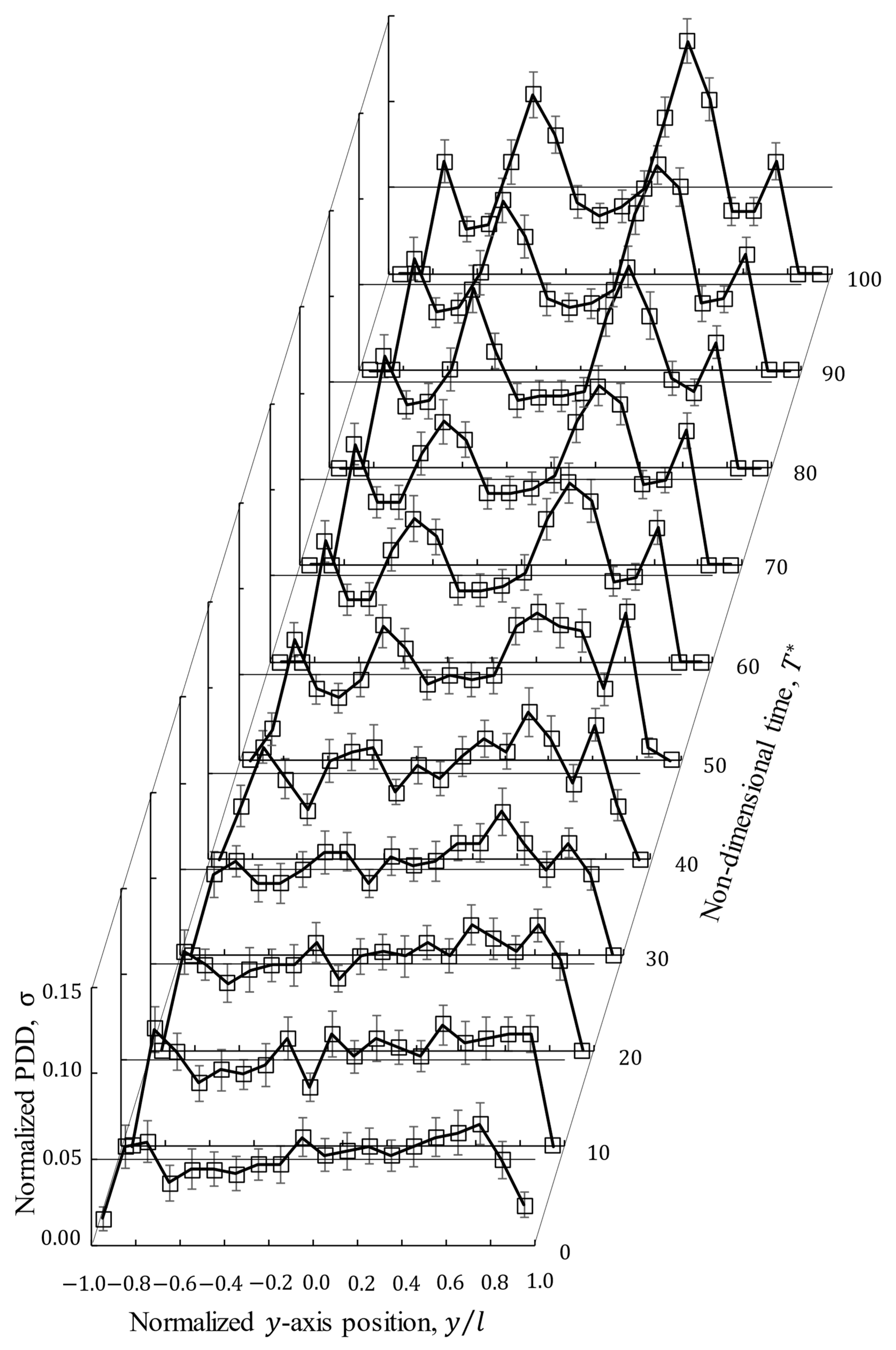
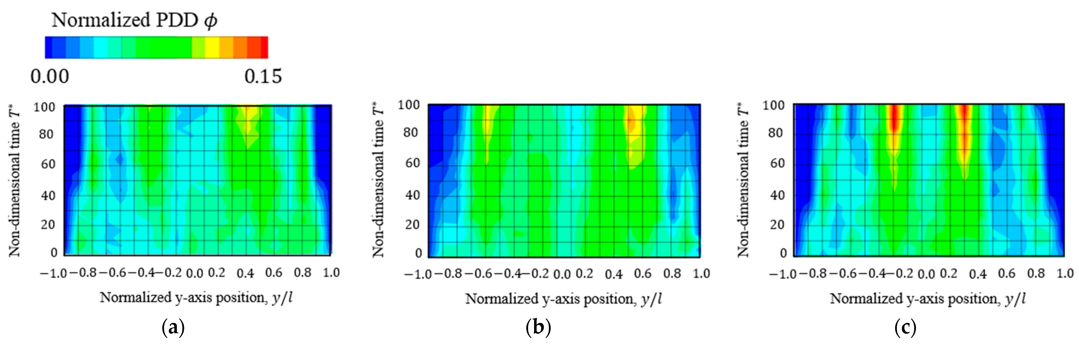
4.1. Concentration Profile

To examine the behavior of multiple particles in a two-dimensional parallel-plate flow, we evaluated the particle density distribution (PDD) [25]. PDD refers to the distribution of particle concentration, defined as the total area occupied by particles in the flow path relative to the total area of the flow path, which is divided into 20 sections along the width.

The normalized change in PDD over time for a power-law index $n=1.0$—where the solvent portion of the suspension behaves as a Newtonian fluid—is shown in Figure 6 at intervals of $T^{*}=10$. Here, $T^{*}=D/U$ represents non-dimensional time. The solid line in the figure represents a homogeneous dispersion state at $0.5$. Additionally, Figure 6 shows that at $T^{*}=0$, the PDD is nearly flat, indicating that the particles are evenly distributed across the width of the channel.

Figure 7 shows a color map of the normalized PDD for various power-law indices. In this map, green represents homogeneous particle dispersion, blue indicates solvent layers, and red signifies areas of particle accumulation. The observed trends are consistent across all power-law indices. Over time, particles migrate toward the channel center, accumulating at two points symmetrical to the center and disappearing near the walls. Moreover, as the power-law index increases, the accumulation shifts closer to the channel center, whereas, with a smaller power-law index, the accumulation occurs nearer to the walls.

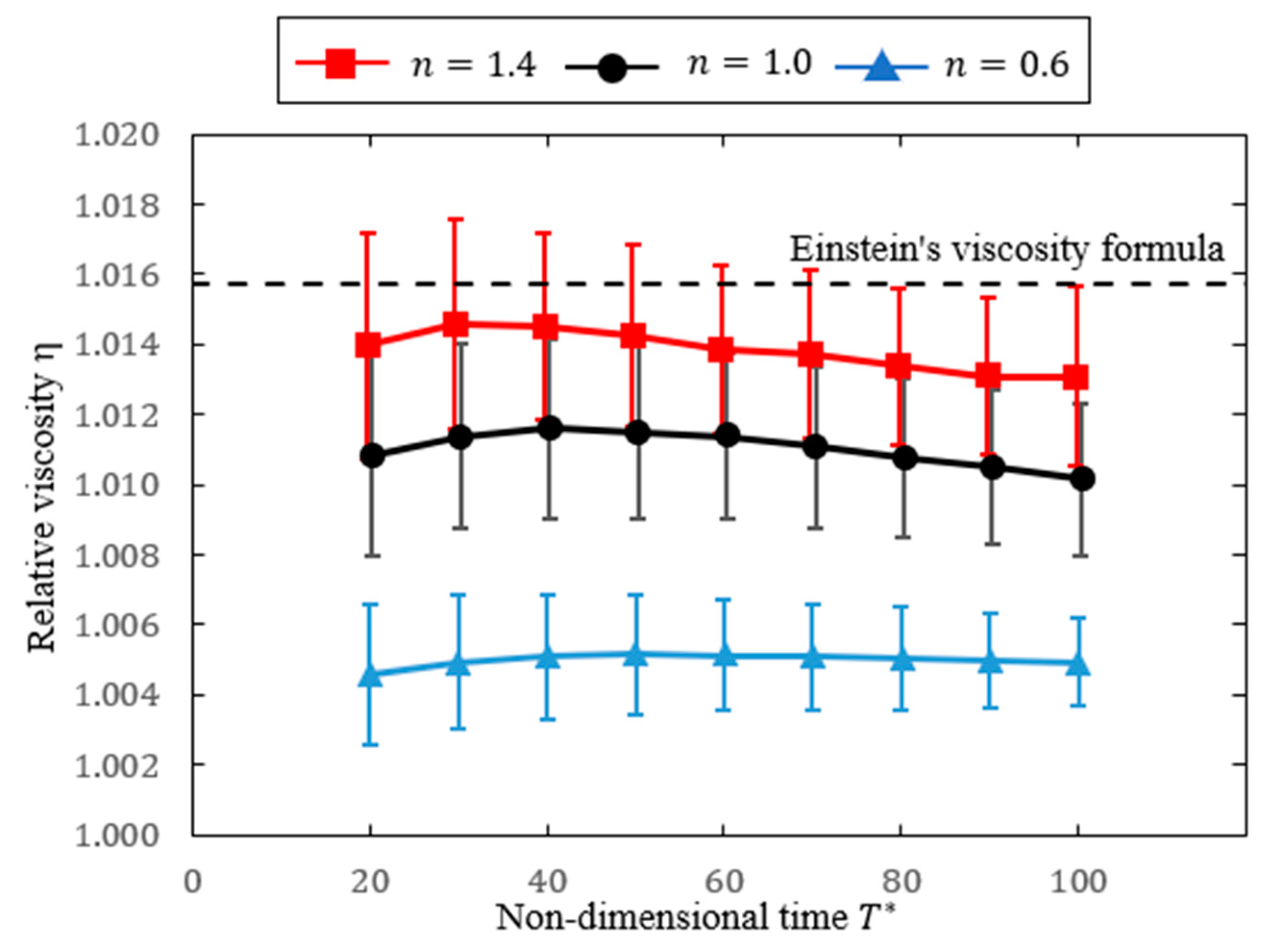
4.2. Relative Viscosity

To examine the rheology of suspensions in a two-dimensional parallel-plate flow, evaluations were performed based on relative viscosity. Figure 8 shows the average of 24 analyses of the time history of relative viscosity. The blue, black, and red colors correspond to power-law indices $n=0.6, 1.0, 1.4$, respectively, while the error bars indicate the standard deviations. The black dotted line represents the results from Einstein’s viscosity formula for this concentration.

The relative viscosity shows similar trends across all power-law indices, and its values are lower than those predicted by Einstein’s viscosity formula. It increases during the non-dimensional time $T^{*}$ = 20–30, and decreases thereafter. During $T^{*}$ = 20–30, the calculated condition is impact departure, leading to an increase in relative viscosity owing to the rise in shear rate. The reasons for the decrease in relative viscosity after $T^{*}=40$ are discussed below.

According to previous studies, Doyeux et al. [12] proposed that macroscopic relative viscosity could be expressed as the sum of individual particle contributions, which depend on their relative positions in the channel. When particles flow near the wall, the relative viscosity increases, even under the same concentration conditions. This phenomenon was also noted by Okamura et al. [13], who indicated that relative viscosity could be estimated by summing the contributions of each particle. As observed in Figure 7 and Figure 8, it can be inferred that the relative viscosity decreases over time as particles migrate toward the center. This microscopic inertial migration of particles in the suspension results in the observed changes in macroscopic relative viscosity.

Here, we present the results for the power-law index $n=1.4$, regarding the time history of relative viscosity. A fluid characterized by a power-law index $n=1.4$ demonstrates shear-thickening behavior. When the solvent of the suspension is a Newtonian fluid, the viscosity can be predicted by the Einstein viscosity formula, but when the solvent is shear-thickening, the suspension’s overall viscosity will also be influenced by shear-thickening effects. Therefore, one would expect the relative viscosity of the suspension to exceed that predicted by Einstein’s viscosity formula. However, the findings show a deviation from this expectation, with the relative viscosity being lower than Einstein’s prediction. This discrepancy may be attributed to the inertial migration of particles, the presence of a non-Newtonian solvent, and particle–particle interactions, none of which are accounted for in Einstein’s viscosity formula. Among these factors, the loss of particles near the walls owing to inertial migration is believed to considerably influence the reduction in relative viscosity. In other words, it appears that the microstructure has a more substantial effect on the flow characteristics of the suspension than the properties of the solvent. Therefore, monitoring changes in the microstructure using PDD is valuable for predicting the flow characteristics of the suspension.

5. Conclusions

In this study, we investigated how the power-law index $n$ of the solvent affects the rheology of a suspension by numerically analyzing a non-Newtonian fluid in a two-dimensional parallel-plate flow. The results for PDD indicate that particles migrate toward the center of the channel owing to inertial effects, with their accumulation becoming increasingly concentrated near the center as the power-law index increases.

The time history results of the relative viscosity show that the microscopic migration of particles results decreases the macroscopic relative viscosity. Moreover, even when the power-law index $n$ is above 1, and the solvent exhibits shear thickening, the apparent viscosity decreases, owing to the inertial migration of particles. Consequently, the relative viscosity falls below the value predicted by Einstein’s viscosity formula, indicating that the suspension behaves in a shear-thinning manner. Therefore, it can be concluded that changes in the microstructure of the suspension have a more considerable influence on its flow characteristics than the properties of the solvent. As a result, the microscopic particle positions obtained through PDD are considered essential for predicting the macroscopic rheology of suspensions.

Finally, this study has several limitations. The two-way coupling scheme places the highest priority on the bidirectionality of suspension flow analysis, and due to its high computational cost, three-dimensional analysis is currently impractical. Therefore, our research group plans to conduct experimental validation.

References

1. Thomas, D.G. Transport characteristics of suspension. A note on the viscosity of Newtonian suspensions of uniform spherical particles. J. Colloid Sci. 1965, 20, 267–277. [Google Scholar] [CrossRef]
2. Matas, J.P.; Morris, J.F.; Guazzelli, É. Inertial migration of rigid spherical particles in Poiseuille flow. J. Fluids Mech. 2004, 515, 171–195. [Google Scholar] [CrossRef]
3. Wen, B.; Chen, H.; Qin, Z.; He, B.; Chang, Z. Lateral migration and nonuniform rotation of suspended ellipse in Poiseuille flow. Comput. Math. 2019, 78, 1142–1153. [Google Scholar] [CrossRef]
4. Gamonpilas, C.; Morris, J.F.; Denn, M.M. Shear and normal stress measurements in non-Brownian monodisperse and bidisperse suspensions. J. Rheol. 2016, 60, 289–296. [Google Scholar] [CrossRef]
5. Einstein, A. Eine neue Bestimmung der Moleküldimensionen. Ann. Phsik 1906, 324, 289–306. [Google Scholar] [CrossRef]
6. Brady, J.F. The Einstein viscosity correction in n dimensions. Int. J. Multiph. Flow 1984, 10, 113–114. [Google Scholar] [CrossRef]
7. Stickel, J.J.; Powell, R.L. Fluid mechanic rheology of dense suspensions. Annu. Rev. Fluid Mech. 2005, 37, 129–149. [Google Scholar] [CrossRef]
8. Morris, J.F. A review of microstructure in concentrated suspensions and its implications for rheology and bulk flow. Rheol. Acta 2009, 48, 909–923. [Google Scholar] [CrossRef]
9. Segré, G.; Silberberg, A. Radial particle displacements in Poiseuille flow of suspensions. Nature 1961, 189, 209–210. [Google Scholar] [CrossRef]
10. Zhang, J.; Li, W.; Alici, G. Inertial Microfluidics: Mechanisms and Applications. Lab Chip 2009, 9, 563–587. [Google Scholar]
11. Inamuro, T.; Maeda, K.; Ogino, F. Flow between parallel walls containing the lines of neutrally buoyant circular cylinders. Int. J. Multiph. Flow 2000, 26, 1981–2004. [Google Scholar] [CrossRef]
12. Doyeux, V.; Priem, S.; Jibuti, L.; Farutin, A.; Ismail, M.; Peyla, P. Effective viscosity of two-dimensional suspension: Confinement effects. Phys. Rev. Fluids 2016, 1, 043301. [Google Scholar] [CrossRef]
13. Okamura, N.; Fukui, T.; Kawaguchi, M.; Morinishi, K. Influence of each cylinder’s contribution on the total effective viscosity of a two-dimensional suspension by a two-way coupling scheme. J. Fluid Sci. Technol. 2021, 16, JFST0020. [Google Scholar] [CrossRef]
14. Hu, X.; Lin, J.; Ku, X. Inertial migration of circular particles in Poiseuille flow of a power-law fluid. Phys. Fluids 2019, 31, 073306. [Google Scholar] [CrossRef]
15. Tomioka, K.; Fukui, T. Numerical Analysis of Non-Newtonian Fluid Effects on the Equilibrium Position of a Suspended Particle and Relative Viscosity in Two-Dimensional Flow. Fluids 2024, 9, 37. [Google Scholar] [CrossRef]
16. Xu, J.; Wang, K.; Li, J.; Zhou, H.; Xie, X.; Zhu, J. ABC Triblock Copolymer Particles with Tunable Shape and Internal Structure through 3D Confined Assembly. Macromolecules 2015, 48, 2628–2636. [Google Scholar] [CrossRef]
17. Yosef, M.; Alex, L. Particle–fluid interaction forces as the source of acceleration PDF invariance in particle size. Int. J. Multiph. Flow 2015, 76, 22–31. [Google Scholar]
18. Izham, M.; Fukui, T.; Morinishi, K. Application of regularized lattice Boltzmann method for incompressible flow simulation at high Reynolds number and flow with curved boundary. J. Fluid Sci. Technol. 2011, 6, 812–822. [Google Scholar] [CrossRef]
19. Fukui, T.; Kawaguchi, M.; Morinishi, K. A two-way coupling scheme to model the effects of particle rotation on the rheological properties of a semidilute suspension. Comput. Fluids 2018, 173, 6–16. [Google Scholar] [CrossRef]
20. Tanno, I.; Morinishi, K.; Matsuno, K.; Nishida, H. Validation of virtual flux method for forced convection flow. JSME Int. J. Ser. B 2006, 49, 1141–1148. [Google Scholar] [CrossRef]
21. Morinishi, K.; Fukui, T. An Eulerian approach for fluid-structure interaction problems. Comput. Fluids 2012, 65, 92–98. [Google Scholar] [CrossRef]
22. Kawaguchi, M.; Fukui, T.; Morinishi, K. Comparative study of the virtual flux method and immersed boundary method coupled with regularized lattice Boltzmann method for suspension flow simulations. Comput. Fluids 2022, 246, 105615. [Google Scholar] [CrossRef]
23. Adachi, H.; Fukui, T. Comparative Study of boundary treatment schemes in lattice Boltzmann method. J. Fluid Sci. Technol. 2024, 19, JFST0025. [Google Scholar] [CrossRef]
24. Boyd, J. A second-order accurate lattice Boltzmann non-Newtonian flow model. J. Phys. A Math. Gen. 2006, 39, 14241–14247. [Google Scholar] [CrossRef]
25. Fukui, T.; Kawaguchi, M. Numerical study of microscopic particle arrangement of suspension flow in a narrow channel for the estimation of macroscopic rheological properties. Adv. Powder Technol. 2022, 33, 103855. [Google Scholar] [CrossRef]
Figure 1. A schematic of the computational model showing circular rigid particles suspended in a two-dimensional channel with random distribution.
Processes 13 00690 g001
Figure 2. D2Q9 model.
Processes 13 00690 g002
Figure 3. Schematic of virtual flux method.
Processes 13 00690 g003
Figure 4. Schematic diagram of particle-free flow in two-dimensional channel.
Processes 13 00690 g004
Figure 5. Velocity profile of particle-free flow in two-dimensional channel for different power-law indices.
Processes 13 00690 g005
Figure 6. Normalized PDD change over time for n = 1.0 , R e = 256 and ϕ = 0.79 . Data are represented as mean ± standard deviation.
Processes 13 00690 g006
Figure 7. Normalized PDD for different power-law indices. (a) n = 0.6 , (b) n = 1.0 , and (c) n = 1.4 .
Processes 13 00690 g007
Figure 8. Relative viscosity changes over time for different power-law indices n = 0.6 ,   1.0 ,   1.4 . Black dotted line represents Einstein’s viscosity formula.
Processes 13 00690 g008