Abstract
Fault detection, classification, and precise location identification in power transmission lines are critical issues for energy transmission and power systems. Accurate fault diagnosis is essential for system stability and safety as it enables rapid problem resolution and minimizes interruptions in electrical energy supply. The characteristic parameters of mixed-conductor power transmission lines connected to the grid were calculated using the relevant line data. Based on these parameters, a dataset was created with computer-derived values. This dataset included variations in arc resistance and the short circuit power of the corresponding bus, facilitating the performance testing of various machine learning algorithms. It was observed that the correct determination of the faulty phase was of high importance in the correct determination of the fault position. For this reason, a gradual structure was preferred. It was achieved with a 100 percent success rate in fault detection with the ensemble bagged algorithm. It was obtained with the neural network algorithm with a 99.97 percent success rate in faulty phase detection. The most successful location results were obtained with the interaction linear algorithm with 0.0066 MAE for phase-to-phase faults and the stepwise linear algorithm with 0.0308 MAE for phase ground faults. Using the proposed algorithm, fault locations were identified with a maximum error of 26 m for phase-to-ground faults and 110 m for phase-to-phase faults on a transmission line with a mixed conductor of approximately 178 km. Additionally, we compared the training and testing results of several machine learning algorithms metrics including the accuracy, total error, mean absolute error, root mean square, and root mean square error to provide informed recommendations based on their performance. The findings aim to guide users in selecting the most effective machine learning models for predicting failures in transmission lines.
1. Introduction
Electricity is one of the most significant discoveries in human history, with a wide range of applications across various sectors such as automotive, tourism, information technology, industry, and medicine. In line with technological advancements, the demand for electrical energy is expected to grow day by day. To meet this increasing energy demand, countries are working to modernize and expand their grid infrastructure [1].
The transmission of electrical energy from production units to consumption units occurs through electrical power systems. The energy transmission line (TL), responsible for transferring energy between electricity generation centers and consumers, forms the backbone of these power systems [2]. The role of electrical energy system management is to ensure the continuous, reliable, stable, and high-quality transmission of electrical energy. Furthermore, it must remain environmentally conscious and operate in alignment with the relevant energy policies [1,2].
Limiting the damage that may be caused by a system fault that will occur in any of the grid elements is of great importance for the stability and security of the electrical energy systems. The accurate diagnosis of faults is crucial for energy transmission and power systems as it enables the swift elimination of issues to minimize interruptions in electric energy [3]. Therefore, getting more accurate information about the fault will speed up the maintenance and commissioning of the defective TL [4]. The numerical distance relays in use today play a key role in isolating the part where the fault is located from the network by detecting the fault of the TL or network elements and initiating the appropriate protection action [5].
The overcurrent protection function becomes inadequate due to fluctuations in the short circuit current of the corresponding bus bar within the electrical system. To address this issue, distance protection relays utilize additional information, including the transmission line’s characteristic data and detailed current and voltage measurements during faults [6]. For this reason, distance protection relays are widely used in ring networks. However, with the continuously growing energy demand, the node points in the electrical system are increasing in number and complexity. Insufficient or inaccurate data used in distance protection relays can compromise their performance, making it difficult to detect faults accurately and reliably [7]. Factors such as incomplete measurements, errors in current and voltage readings, or missing environmental and system parameters can increase the likelihood of malfunctions or disoperation. Numerical distance protection relay algorithms for lines with different characteristic features because of the internal and external disruptive effects may not reduce the error rate of fault classification and location below a certain value.
Today, the concept of a smart grid is gradually evolving, aiming to establish an intelligent system capable of monitoring, controlling, and diagnosing failures effectively. Advances in areas such as measurement transformers with a lower fault tolerance, more sophisticated digital signal processing technology, and artificial intelligence provide an opportunity for researchers to conduct in-depth research on fault detection and location information in the TL [8,9,10].
Due to its potential to greatly increase the accuracy of fault identification and classification, machine learning (ML) has drawn a lot of attention recently for use in TL fault detection [11,12,13]. Numerous ML algorithms, such as ensemble, decision trees, support vector machines, artificial neural networks, and linear and Gaussian models, have undergone extensive research and testing. These algorithms analyze current and voltage signals to identify TL faults and could provide more accurate information about the location and classification of faults. The efficiency of ML techniques in producing accurate predictions for fault classification and fault location has been confirmed by numerous studies.
A study was conducted to use wavelet packet entropy and a radial basis function neural network to detect, classify, and estimate fault locations on transmission lines. The radial basis function neural network had 12 inputs, used a Gaussian radial basis function as its activation function, and achieved a classification accuracy of about 98%. However, the accuracy varied depending on the fault type, with some line ground faults having lower accuracy (~93%) [14].
In a study conducted to estimate fault locations in 154 kV hybrid transmission lines, which include both overhead and underground cable sections, the author used PSCAD software to obtain the necessary data. The most accurate fault location estimation was performed using robust linear regression, with a maximum observed error of 2.4 km [12].
A study was conducted to develop a discrete wavelet transform-based algorithm to detect, classify, and locate faults on high-voltage transmission lines. The method used the Daubechies 6 wavelet for analysis and a ground threshold value for classification. Faults were identified across the entire transmission system, from one terminal to the other. The algorithm successfully handled all 11 types of TL faults by analyzing signal details and locating faults using the discrete wavelet transform technique [15].
Another study realized a new approach that integrated neural networks with distance relays to improve fault location accuracy in transmission lines. This integration significantly reduced the average fault location error of the distance relay from 0.92% to 0.42%, resulting in a significant improvement in accuracy [16].
A method utilizing Elman neural networks was developed to detect failures in power transmission lines. This study leveraged the strong learning capabilities of Elman neural networks to accurately classify and identify faults. Based on the conducted tests and simulations, the proposed method was shown to achieve an error detection accuracy of 82.4% [8].
Another study evaluated three ML classifiers decision tree, K-nearest neighbor, and support vector machine for detecting faults in TL. Among these, decision tree achieved the highest accuracy of 99.42%, followed by K-nearest neighbor at 99.27% and support vector machine at 87.03%. Additionally, the authors combined Discrete Wavelet Transform with support vector machine for fault detection, achieving a fault classification accuracy of 99.4% and a fault detection error of less than 1.5%. The primary goal of the study was to propose an ensemble method for efficient fault detection and classification in TL [9].
The characteristic parameters of energy TL with mixed conductors (954 MCM and 1272 MCM) connected to the grid within the interconnect system were analyzed. Based on these parameters, a dataset was created with Omicron Test Universe 4.40 and Digsilent PowerFactory 01/2024 software. This dataset included variations in arc resistance and the short circuit power of the corresponding bus, facilitating the performance testing of various machine learning algorithms.
In this paper, we proposed a cascade of machine learning algorithms achieving the best results with the ensemble method for fault detection, the neural network method for identifying faulty phases, and linear regression for precise location identification. It was observed that the correct determination of the faulty phase was of high importance in the correct determination of the fault position. For this reason, a gradual structure has been preferred. It has been achieved with a 100 percent success rate in fault detection with the ensemble bagged algorithm. It was obtained with the neural network algorithm with a 99.97 percent success rate in faulty phase detection. The most successful location results were obtained with the interaction linear algorithm with 0.0066 MAE for phase-to-phase faults and the stepwise linear algorithm with 0.0308 MAE for phase ground faults. Using the proposed algorithm, fault locations were identified with a maximum error of 26 m for phase-to-ground faults and 110 m for phase-to-phase faults on a transmission line with a mixed conductor of approximately 178 km. Additionally, we compared the training and testing results of several machine learning algorithms metrics including the accuracy, total error, mean absolute error, root mean square, and root mean square error to provide informed recommendations based on their performance. The findings aim to guide users in selecting the most effective machine learning models for predicting failures in transmission lines. The characteristic parameters of the TL are summarized in Table 1, providing detailed information on the line’s properties and specifications.

Table 1.
The characteristic parameter details of the tested power transmission line.
2. Distance Protection Relays
Distance protection relays are widely used to accurately, quickly, and selectively detect and analyze faults in TL. Distance protection involves identifying the fault location by utilizing the transmission line’s characteristic data and measured current and voltage information, processed through specific algorithms. In simple terms, distance relays calculate impedance using current and voltage measurements [2,17]. They then determine the presence of a fault by comparing the calculated impedance with the TL predefined impedance value. Figure 1 illustrates the connection of the distance protection relay to the system, showing how it connects with the current and voltage transformers. This connection ensures that the relay receives accurate real-time data for fault detection and analysis [18].
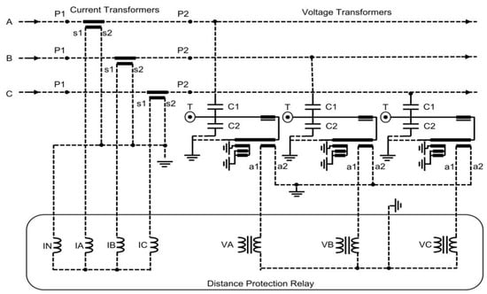
Figure 1.
Distance protection relay connection diagram.
Single-phase-to-ground faults are the most common type of fault in power systems, accounting for approximately 85% of all fault types [19]. The oscillographic representation in Figure 2a illustrates the measured variations in current and voltage for each phase during a single-phase ground short circuit event in the electrical system. A decrease in phase B voltage and an increase in its current indicate a fault in phase B. The similarity between phase B current and neutral current shows a B-phase-to-ground fault.
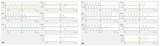
Figure 2.
Oscillographic record of the feeder when faults occur (a) for a B-phase ground fault and (b) for an AC-ground fault.
A two-phase ground fault is a critical type of fault in electrical power systems and usually results in more complex effects. The difference from single-phase-to-ground failure is that two phases come into contact with the ground at the same time [20,21]. This can lead to bigger fault current. In Figure 2b a voltage drop and current increase in phases A and C indicate a malfunction in these phases, while a partial voltage rise in phase B and fault current in the neutral suggest that the fault occurred in the ACN phases.
A phase-to-phase fault is a type of fault that occurs when two phases of a power system come into direct contact with each other, typically due to a short circuit. In this case, there is zero impedance between the two phases involved in the fault, which means the fault path offers no resistance, leading to an extremely high current flow [22,23]. This accounts for approximately 8% of all fault types [19]. The oscillographic representation in Figure 3a illustrates the measured variations in current and voltage for each phase during a phase-to-phase short circuit event in the electrical system. The fault current between phases A and B has a 180-degree phase difference. The decrease in A and B phase voltages, along with the impedance dropping below the threshold, indicates an A-B phase fault.
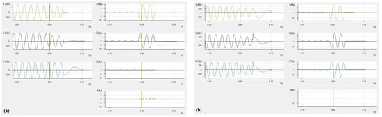
Figure 3.
Oscillographic record of the feeder when fault occur (a) for AB fault and (b) for ABC fault.
A three-phase fault represents one of the most severe disturbances that can occur within a power system. It involves the simultaneous short circuiting of all three phases, either directly or through an arc resistor. This type of fault is distinguished by its exceptionally high fault current magnitudes, posing significant challenges to the stability of the system [24]. The oscillographic representation in Figure 3b illustrates the measured variations in current and voltage for each phase during a three-phase short circuit event in the electrical system. The voltage and current in phases A, B, and C exhibit similar characteristics. With impedance below the threshold and no fault current in the neutral, this indicates a typical three-phase short circuit fault.
Distance protection relays typically consist of three main units: the measuring unit, initiation unit, and directional unit, each performing specific tasks. These relays provide selective protection, which relies on the proper functioning of all three units. Regardless of their structure, distance protection relays operate by comparing impedance values. Using the formula, the relay calculates the line’s impedance [18,25]. During a fault, the voltage decreases while the current increases, resulting in a lower measured impedance than under normal conditions [17,26]. The relay identifies the fault by comparing the measured impedance with a predefined threshold. The impedance value measured by the relay depends on the distance between the relay and the fault location. Theoretically, the impedance is directly proportional to the line length. If the measured impedance is lower than the relay’s set threshold, the relay initiates the start chain. It then determines whether to issue a trip command based on the fault current’s direction and distance [18].
Distance Protection Relay Fault Locator Working Principle
Impedance measurement is performed for each phase by the distance protection relay, and the fault type and related phases or phases are determined after the fault is detected. The calculation algorithm to be used in the relay is selected according to the determined fault type [21,26]. For example, a phase-to-phase cycle is preferred for fault detection in phase-to-phase short circuits. In the case of a single-phase earth short circuit, calculations are made by taking into account the value of the impedance of the earth-return path to calculate the single phase to earth cycle. Determination of the fault location in distance protection relays is based on the evaluation of the imaginary part of the measured short circuit impedance. The fault location is determined by dividing the calculated reactance value by the parameterizable reactance per unit length [17,18]. Figure 4 shows the situation before and during the fault.
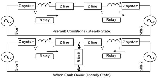
Figure 4.
Prefault and fault conditions (steady state).
In Equation (1) below, and represent the short circuit voltage phasors for phases B and C, respectively. and represent the short circuit current phasors for phases B and C, respectively. The proportional distance to the fault location (m) represents the relative position of a fault location along the length of a TL in terms of Z, which represents line impedance. Figure 5 represent the voltage change when fault occurs.
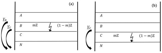
Figure 5.
Voltage change when fault occurs at a distance m (a) for BC ground fault and (b) for C-N fault.
The equation used by the protection element to calculate the short circuit impedance occurring between the B and C phases is given in Equation (1).
represents the short circuit soil resistance, and the fault resistance RBC and fault inductance XBC represent the fault location for the phase-to-phase fault in Equations (2) and (3) [18].
The equation used by the protection element to calculate the short circuit impedance occurring between the C and N phases is given in Equation (4). represents the short circuit current phasors for phases N.
In Equations (5) and (6), and represent the auxiliary quantity. The factors and are obtained solely from the TL constants.
In this case, the line resistance and inductance represent the fault location for the phase-to-ground fault in Equations (7) and (8) [18].
3. Types of Machine Learning Algorithms Used for Classification and Regression
This section offers an overview of the machine learning algorithms employed, highlighting their key features and functionalities.
3.1. Linear Regression
Linear regression is a statistical and ML technique used to estimate the value of an unknown (dependent) variable based on the value of a known (independent) variable. It establishes a relationship between the two variables by modeling them mathematically as a linear equation [27,28].
where y is the dependent variable (the response or predicted value); x is the independent variable (the predictor or input); m is the slope of the line, representing the rate of change of y with respect to x; and b is the intercept, representing the value of y when x = 0.
Linear regression assumes a linear relationship between variables and minimizes the sum of squared errors to find the best fit line. It is widely used for prediction and trend analysis [29].
3.2. Logistic Regression
Logistic regression is a statistical method used to analyze the cause–effect relationship between independent variables and a dependent variable (class variable) that has two or more categories. It builds a classification model using the existing data by estimating the probability of an observation belonging to a particular class. Then it determines the strength and significance of the relationship between the independent variables and the dependent variable [30].
In logistic regression analysis, the importance of these relationships is assessed by examining the significance of the coefficients of the independent variables. Additionally, the model evaluates how well the predicted values match the observed values for the cases where the variable of interest is present in the model. This comparison helps to assess the model’s accuracy and its ability to classify data correctly [31,32].
3.3. Gaussian Process
Gaussian process regression (GPR) is a fully probabilistic approach for modeling nonlinear relationships between variables. It provides not only predictions but also uncertainty estimates for those predictions, making it a powerful tool for regression tasks.
In the Bayesian framework, GPR can be enhanced for robustness by employing heavy-tailed distributions to model noise instead of the standard normal distribution. Heavy-tailed distributions are less sensitive to outliers because they assign lower probabilities to extreme deviations compared with normal distributions [33]. This makes the model more robust in scenarios where the data may include noise or outliers that would otherwise significantly affect the predictions. GP regression is particularly suitable for small to medium-sized datasets, where the computation of covariance matrices remains manageable. Its flexibility and probabilistic nature make it a valuable tool for understanding complex, uncertain systems [34].
3.4. K-Nearest Neighbors
K-nearest neighbors (K-NN) is a classification method that assigns an unclassified instance to a class based on its distance from previously classified data points. The algorithm evaluates the distances between the unclassified instance and all known data points, identifies the K-NN, and assigns the instance to the class most common among those neighbors [35,36]. This method relies heavily on the chosen distance metric and the value of K, which determines the number of neighbors considered [7,36,37].
3.5. Ensemble Methods
Ensemble ML is defined as an element of a set of classifiers in which individual decisions are combined to classify new examples to be experienced. This technique aims to achieve more powerful and effective results by combining the answers of ML algorithms with different characteristics. The main purpose of ensemble ML is to enable it to make more accurate predictions by analyzing a large number of data that have different characteristics. Due to the fact that individual classifiers make independent errors, the collection of a composite multi-classifier in order to minimize the error rate can increase the classifier accuracy [38].
3.6. Neural Networks
Neural networks (NNs) are inspired by the functioning of human and animal brains. They are designed with a large number of interconnected processing elements (artificial neurons) that mimic the elementary functions of biological neurons [39]. They learn by adjusting the weights of connections based on experience, allowing the system to generalize from past experiences to handle new, unseen scenarios [16].
NNs focus on learning patterns and relationships from previously acquired data, referred to as training or learning datasets. Then, they improve and evaluate the performance of the system using the test data. In addition, NNs are versatile tools capable of handling complex problems [9,39].
3.7. Decision Trees
The decision tree algorithm works by recursively dividing the dataset into smaller and smaller subsets, ultimately forming a hierarchical structure. Each decision node in the tree represents a test on a feature, with branches corresponding to the possible outcomes of the test. The process begins at the root node, which is the topmost node in the tree [40].
Decision trees are nonparametric, distribution-independent methods used in supervised learning tasks. Their structure mimics a tree, consisting of root nodes, branches, and leaves. The leaf nodes represent the output, which can be either a class label for classification problems or a numerical value for regression problems [41].
The complexity of the dataset significantly impacts the decision tree’s structure. If the data are intricate, the tree grows deeper and more branched, potentially leading to overfitting. As a result, decision trees are sensitive to the quality of the dataset and may require pruning or other optimization techniques to improve generalization [40].
3.8. Naive Bayes
Naive Bayes is a statistical classification algorithm that estimates the probability of an instance belonging to a particular class. It is based on Bayes’ theorem and, unlike many other learning methods, calculates the likelihood of various combinations of features in the training data. This algorithm assumes that the features are independent of each other [41,42].
The naive Bayes algorithm operates using finite probability calculus, making it computationally efficient and well suited for high-dimensional datasets. Despite the independence assumption, it often performs surprisingly well in practical applications, especially in text classification, spam filtering, and sentiment analysis [43].
3.9. Support Vector Machine
Support vector machine (SVM) is a supervised learning algorithm that constructs a hyperplane or a set of hyperplanes in high- or infinite-dimensional spaces to separate data into distinct classes [44]. The algorithm seeks to maximize the margin, which is the distance between the hyperplane and the nearest data points from each class (support vectors). A larger margin generally leads to lower generalization error and better classification performance. SVM is particularly effective in high-dimensional spaces, making it suitable for complex datasets [45,46].
4. Implementation and Performance Review
4.1. Preparing Dataset for ML Algorithms
It has been observed that the error rate of the fault location increases if it is included in the same dataset with conditions in which there is no fault. For this reason, three different algorithm structures working in series were preferred to obtain the most accurate result:
- Fault detection;
- Fault phase detection;
- Fault location detection.
The current and voltage of each phase were constantly monitored. If a fault occurred and if the fault current was above the specified threshold value, it was detected by the fault detection algorithms. The fault classifying algorithms evaluated the resistance and inductance values of each phase as input, and it determined which phase or phases had a fault. Then, regression algorithms using the resistance and inductance values of the relevant phases determined the fault position depending on which phase or phases the fault occurred from. This situation is summarized in the flowchart diagram in Figure 6.
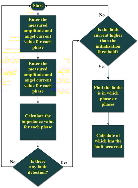
Figure 6.
Flowchart for the proposed methodology in fault classification and location.
The dataset was created with the assumption that the analog data from the current and voltage transformers were accurate. There were records in the dataset with the same fault location but different fault currents and fault arc resistance. These cases were added to reflect the potential impact of multiple fault scenarios or changes in fault conditions at the same location. In Table 2, a fault status is indicated by a value of 1 in the fault detection column. A binary system adaptation is applied to the phase detection column for encoding faults. For instance, the ABC fault in the first two rows is encoded as 8 + 4 + 2 + 0 = 14, while the AB-N fault is encoded as 8 + 4 + 0 + 1 = 13. This encoding method is used to facilitate fault detection. Impedance information for each phase was obtained using the Omicron Test Universe and Digsilent programs, based on the characteristic properties provided in Table 1 for the fault location dataset. A sample from the dataset used during the testing and validation steps of the ML algorithms is presented in Table 2.
Table 2.
Fault, faulty phase, and location dataset.
4.2. Performance Criteria for Precise Fault Location
The assessment of the models employed in this study was conducted using three distinct performance metrics to comprehensively evaluate the accuracy and effectiveness of the predicted outcomes.
4.2.1. Mean Absolute Error
The mean absolute error (MAE) quantifies the deviation between the predicted values, generated by the models, and the actual observed values [47,48]. The formal definition of MAE is provided in Equation (10).
In Equation (10), denotes the actual value of the variable being estimated; represents the corresponding predicted value; and reflects the residual, or the difference between the observed and predicted values.
4.2.2. Mean Squared Error
The mean squared error (MSE) represents the average of the squared differences between the predicted values and the actual observed values, as defined in Equation (11) [49].
4.2.3. Root Mean Squared Error
The root mean squared error (RMSE) is calculated by taking the square root of the MSE, as expressed in Equation (12) [48].
4.3. Findings
4.3.1. Fault Detection
Initially, the fault condition was identified by analyzing the resistance and inductance values of the three phases. The dataset contained 12,768 samples, with half representing the fault state and the other half representing the non-fault state. The dataset was divided into two subsets: 65% was utilized as validation data, while the remaining 35% was allocated for testing. Figure 7a,b show the validation and test confusion matrix of the ensemble bagged trees method.
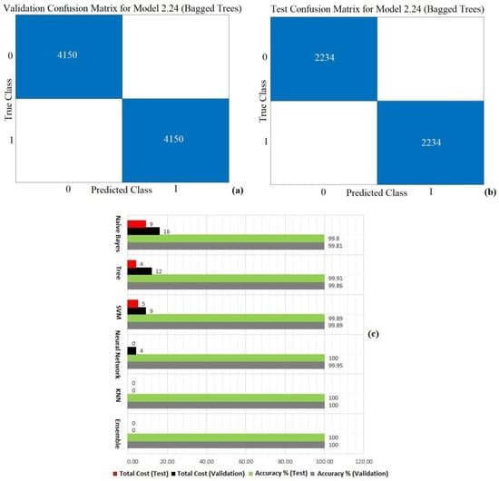
Figure 7.
(a) Confusion matrix for fault detection ensemble bagged trees, validation. (b) Confusion matrix for fault detection ensemble bagged trees, test. (c) Accuracy and total cost value for the ensemble, KNN, NN, SVM, tree, and naive Bayes algorithms.
The accuracy and test results for the ML algorithms used in the analysis are summarized below. The evaluation included validation accuracy, test accuracy, and other relevant performance indicators to assess the effectiveness of the algorithms in identifying fault conditions. Specific values and comparisons for each algorithm are detailed. As illustrated in the Figure 7c, the K-nearest neighbor and ensemble bagged trees algorithms achieved a perfect adaptation to the dataset, demonstrating 100% accuracy in both training and testing phases.
4.3.2. Faulty Phase Detection
Then an algorithm was developed to detect the faulty phase or phases within the system. The dataset contained 12,768 samples, and each failure category contained nearly 908 samples to ensure balanced representation across the dataset. The dataset was divided into two subsets: 67% was utilized as validation data, while the remaining 33% was allocated for testing. Figure 8a,b show the validation and test confusion matrix of the trilayered NN method.
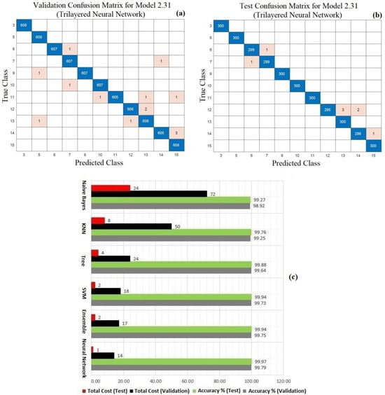
Figure 8.
(a) Confusion matrix for faulty phase detection trilayered neural network, validation. (b) Confusion matrix for faulty phase detection trilayered neural network, test. (c) Accuracy and total cost value for the NN, ensemble, SVM, tree, KNN, and naive Bayes algorithms.
Among the results obtained, the performance of six algorithms, selected from 33 different models, demonstrated the highest prediction accuracy. When the errors made by the trilayered NN algorithm, which was the most successful, were analyzed, it was observed that the highest error rate occurred in three-phase-to-ground faults for validation and AB phase for testing. The accuracy and test results for the ML algorithms used in the analysis are depicted in Figure 8c. These results were summarized, highlighting their effectiveness in identifying the faulty phases. The evaluation included validation accuracy, test accuracy, and other relevant performance indicators to assess the effectiveness of the algorithms in identifying faulty phases. As illustrated in Figure 8a,b, the trilayered NN algorithm achieved a perfect adaptation to the dataset, demonstrating 99.79% accuracy validation and 99.97% accuracy test.
4.3.3. Fault Location Detection
Finally, the goal was to develop an algorithm capable of predicting the fault location accurately. To achieve this, the algorithm selection was guided by identifying which phase or phases were involved in the fault, ensuring that the method could effectively utilize this information for precise fault location. In addition, different algorithms were used for phase-to-phase and phase-to-ground faults to enhance the accuracy of fault location predictions. The significant increase in the error rate in the location detection of phase-to-ground failures was due to the difference in the corresponding fault soil resistance. For this reason, the accuracy rate was increased by using two different algorithms in the regression step in order to obtain a more accurate fault location.
For Phase-to-Phase and Three-Phase Faults
The MAE, MSE, and RMSE values, derived from both the validation and test datasets, are presented for the five ML algorithms that delivered the most accurate outcomes for phase-to-phase and three-phase failure scenarios. As illustrated in Table 3, the interaction linear regression algorithm achieved a perfect adaptation to the dataset, demonstrating 0.0066 MAE, 0.0001 MSE, and 0.0083 RMSE values for validating. Furthermore, the algorithm proved to be a perfect fit for the dataset, showing 0.0071 MAE, 0.0001 MSE, and 0.0089 RMSE values for testing.
Table 3.
Performance evaluation parameters of regression models for validation and test (phase-to-phase failures).
The residual difference plots of the top three most successful algorithms along the line length of phase-to-phase and three-phase faults, based on test and verification data, are presented in Figure 9. The plots in Figure 9 and the data in Table 3 demonstrate that the developed models achieved highly satisfactory distance predictions for both validation and test data. In addition, it was observed that the interactions in the linear regression model provided the most accurate distance estimates for both validation and test data. Upon a detailed examination of Figure 9a,b, it becomes evident, through the aid of the axes, that the system accurately detected the fault location, with a maximum deviation of 25 m, based on a dataset of 456 data points. Table 4 demonstrates key metrics of phase to phase such as the training time, model size, and prediction speed for the machine learning algorithm. The training time represents the duration needed to train the model, the model size indicates the memory footprint of the trained model, and the prediction speed measures how fast the model can generate predictions on new data.
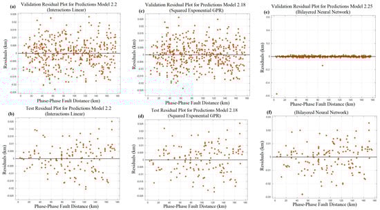
Figure 9.
Residual difference plots at various km points for phase-to-phase failures. (a) Linear regression for validation. (b) Linear regression for testing. (c) Gaussian process for validation. (d) Gaussian process for testing. (e) NN for validation. (f) NN for testing.
Table 4.
Performance evaluation parameters of regression models for phase-to-phase failures.
For Phase-to-Ground Faults
The MAE, MSE, and RMSE values, derived from both the validation and the test datasets, are presented for the five ML algorithms that delivered the most accurate outcomes for phase-to-ground failure scenarios. As illustrated in Table 5, the stepwise linear regression algorithm achieved a perfect adaptation to the dataset, demonstrating 0.0308 MAE, 0.0013 MSE, and 0.0365 RMSE values for validating. Furthermore, the algorithm proved to be a perfect fit for the dataset, showing 0.0319 MAE, 0.0014 MSE, and 0.0372 RMSE values for testing.
Table 5.
Performance evaluation parameters of regression models for validation and test (phase-to-ground failures).
The residual difference plots of the top three most successful algorithms along the line length of phase-to-ground faults, based on test and verification data, are presented in Figure 10. The plots in Figure 10 and the data in Table 5 demonstrate that the developed models achieved highly satisfactory distance predictions for both validation and test data. It was observed that the stepwise linear regression model delivered the most precise distance estimates for the validation dataset, while the squared exponential GPR achieved superior accuracy for the test dataset. Upon a detailed examination of Figure 10a,b, it becomes evident, through the aid of the axes, that the system accurately detected the fault location, with a maximum deviation of 100 m, based on a dataset of 456 data points. The predominant factor contributing to the greater deviation observed in phase-to-ground faults, as opposed to phase-to-phase faults, was the inherent unpredictability of the zero-sequence impedance. Table 6 demonstrates key metrics of phase to ground such as the training time, model size, and prediction speed for the machine learning algorithm.
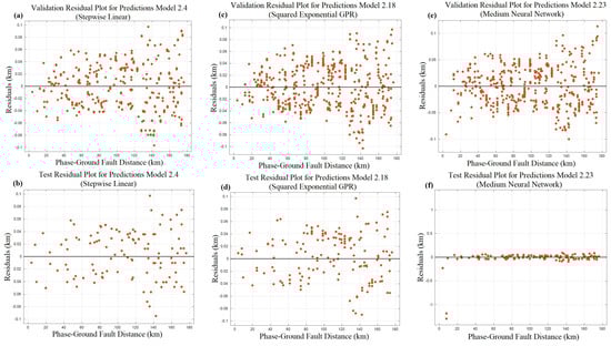
Figure 10.
Residual difference plots at various km points for phase-to-ground failures. (a) Linear regression for validation. (b) Linear regression for testing. (c) Gaussian process for validation. (d) Gaussian process for testing. (e) NN for validation. (f) NN for testing.
Table 6.
Performance evaluation parameters of regression models for phase-to-ground failures.
According to the results presented in Table 7 and Table 8, the prediction percentage errors ranged from a maximum of 98 m to a minimum of 1 m. These outcomes indicated that the algorithm provided a highly accurate fault location prediction as the errors were relatively small and demonstrated the effectiveness of the approach.
Table 7.
Results of fault location prediction for system short circuit currents 25 kA and 35 kA.
Table 8.
Results of fault location prediction for short circuit arc resistances 2 Ω and 10 Ω.
Evaluation of the Overall Performance of the Algorithms Used
It has been observed that models tended to make more errors for phase-earth failures at higher distances (km). The main cause of this was unstable soil resistance. In contrast, for phase-to-phase failures, the error propagation was more uniform. However, on behalf of both cases, due to the presence of two different conductors, failures occurring at these points led to an increased error rate.
The fault location increased in a partially linear relationship with the line’s resistance, and linear regression was well suited to capture this. By preventing overfitting in the dataset, it avoided unnecessary complexity and improved generalization. This reduced the risk of overfitting while yielding more reliable results. Additionally, the feature selection process in linear regression eliminated noise, leading to more stable predictions. All these factors allowed linear regression to perform better on this dataset compared with other algorithms.
5. Conclusions
This study addressed the problem of fault detection, identifying the faulty phase or phases and predicting the exact fault location using various ML algorithms. The primary goal was to achieve more accurate fault detection and classification prediction by developing these classifying algorithms. The ensemble bagged algorithm achieved a 100% success rate in fault detection. The NN algorithm accurately identified faulty phases with 99.97% accuracy. For location estimation, regression algorithms were used, and their performances were compared. To evaluate the algorithms’ performances in validation and testing progress, error residuals were analyzed. The interaction linear algorithm was the most effective for phase-to-phase fault location, 0.0066 MAE, while the stepwise linear algorithm performed best for phase-to-ground faults, 0.0308 MAE. The results demonstrated the effectiveness of the proposed optimization algorithms in improving classification accuracy and more precise fault location definition. Additionally, the study confirmed that the ensemble algorithm exceled in fault detection, the neural network algorithm was superior for fault phase identification, and the linear regression method was the most reliable for precise location prediction.
Future work could explore the integration of deep learning techniques and real-time fault detection systems to further enhance reliability and efficiency. Overall, this research demonstrates the effectiveness of ML-based optimization in improving fault diagnosis in power systems.
Author Contributions
Ö.Ö., R.K., and N.P. contributed to the design and modeling of the system, analysis of the results, and writing of the manuscript. All authors have read and agreed to the published version of the manuscript.
Funding
This research received no external funding.
Data Availability Statement
Data will be made available upon reasonable request. The data are not publicly available due to privacy.
Conflicts of Interest
Author Ömer Özdemir was employed by the company Türkiye Electricity Transmission Company. The remaining authors declare that the research was conducted in the absence of any commercial or financial relationships that could be construed as a potential conflict of interest. The company had no role in the design of the study; in the collection, analyses, or interpretation of data; in the writing of the manuscript, or in the decision to publish the results.
References
- Strielkowski, W.; Civín, L.; Tarkhanova, E.; Tvaronavičienė, M.; Petrenko, Y. Renewable energy in the sustainable development of electrical power sector: A review. Energies 2021, 14, 8240. [Google Scholar] [CrossRef]
- Belu, R. Smart Grid Fundamentals: Energy Generation, Transmission and Distribution; CRC Press: Boca Raton, FL, USA, 2022. [Google Scholar] [CrossRef]
- Jiang, J.; Chuang, C.; Wang, Y.; Hung, C.; Wang, J.; Lee, C.; Member, S.; Hsiao, Y. A hybrid framework for fault detection, classification, and location—Part I: Concept, structure and methodology. IEEE Trans. Power Deliv. 2011, 26, 1988–1998. [Google Scholar] [CrossRef]
- Kumar, S.; Pandey, A.; Goswami, P.; Pentayya, P.; Kazi, F. Analysis of Mumbai Grid Failure Restoration on Oct 12, 2020: Challenges and Lessons Learnt. IEEE Trans. Power Syst. 2022, 37, 4555–4567. [Google Scholar] [CrossRef]
- Fadhel, A.; Tarlochan, S.; Rajiv, V. Performance Comparison of Distance Protection Schemes for Shunt-FACTS Compensated Transmission Lines. IEEE Trans. Power Deliv. 2007, 22, 2116–2125. [Google Scholar] [CrossRef]
- Stefanidou-Voziki, P.; Sapountzoglou, N.; Raison, B.; Dominguez-Garcia, J. A review of fault location and classification methods in distribution grids. Electr. Power Syst. Res. 2022, 209, 108031. [Google Scholar] [CrossRef]
- Vaish, R.; Dwivedi, U.; Tewari, S.; Tripathi, S. Machine learning applications in power system fault diagnosis: Research advancements and perspectives. Eng. Appl. Artif. Intell. 2021, 106, 104504. [Google Scholar] [CrossRef]
- Ertugrul, O.F.; Kurt, M.B. A fast and accurate fault detection approach in power transmission lines by modular neural network and discrete wavelet transform. Comput. Sci. Appl. 2014, 1, 152–157. [Google Scholar]
- Sowah RA Dzabeng, N.A.; Ofoli, A.R.; Acakpovi, A.; Koumadi, K.M.; Ocrah, J.; Martin, D. Design of power distribution network fault data collector for fault detection, location and classification using machine learning. In Proceedings of the IEEE 7th International Conference on Science & Technology (ICAST), Accra, Ghana, 22–24 August 2018; IEEE: Piscataway, NJ, USA, 2018; pp. 1–8. [Google Scholar]
- Hosseini, K. Short circuit fault classification and location in transmission lines using a combination of wavelet transform and support vector machines. Int. J. Electr. Eng. Inform. 2015, 7, 353. [Google Scholar]
- Khan, M.A.; Asad, B.; Vaimann, T.; Kallaste, A.; Pomarnacki, R.; Hyunh, V.K. Improved fault classification and location in power transmission networks using vae-generated synthetic data and machine learning algorithms. Machines 2023, 11, 963. [Google Scholar] [CrossRef]
- Budak, S.; Akbal, B. Fault location estimation by using machine learning methods in mixed transmission lines. Eur. J. Sci. Technol. 2020, 245–250. [Google Scholar] [CrossRef]
- Mukherjee, A.; Kundu, P.K.; Das, A. Transmission line faults in power system and the different algorithms for identification, classification and location a brief review of methods. J. Inst. Eng. India Ser. B 2021, 102, 855–877. [Google Scholar] [CrossRef]
- Patel, B.; Bera, P.; Saha, B. Wavelet packet entropy and RBFNN based fault detection, classification and location on HVAC transmission line. Electr. Power Compon. Syst. 2018, 46, 15–26. [Google Scholar] [CrossRef]
- Saravanababu, K.; Balakrishnan, P.; Sathiyasekar, K. Transmission line fault detection, classification and location using wavelet transform. Int. J. Eng. Adv. Technol. 2019, 8, 1770–1775. [Google Scholar] [CrossRef]
- Linh, H. Integration of neural network and distance relay to improve the fault location on transmission lines. Turk. J. Electr. Eng. Comput. Sci. 2023, 31, 566–580. [Google Scholar] [CrossRef]
- Takagi, T.; Yamakoshi, Y.; Yamaura, M.; Kondou, R.; Matsushima, T. Development of a new type fault locator using the one-terminal voltage and current data. IEEE Trans. Power Appl. Syst. 1982, PAS-101, 2892–2898. [Google Scholar] [CrossRef]
- Siemens Distance and Line Differential Protection Breaker Management for 1-Pole and 3-Pole Tripping 7SA87, 7SD87, 7SL87, 7VK87. 2020 Manual. Available online: https://support.industry.siemens.com/cs/attachments/109742440/SIP5_7SA-SD-SL-VK-87_V09.90_Manual_C011-Q_en.pdf (accessed on 6 February 2025).
- Nhan, N.; Van, L. Fault identification, classification, and location on transmission lines using combined machine learning methods. Int. J. Eng. Technol. Innov. 2022, 12, 91–109. [Google Scholar] [CrossRef]
- Kumari, S.; Mishra, A.; Singhal, A.; Dahiya, V.; Gupta, M.; Gawre, S.K. Fault detection in transmission line using ANN. In Proceedings of the IEEE International Students Conference on Electrical, Electronics and Computer Science (SCEECS), Bhopal, India, 18–19 February 2023; pp. 1–5. [Google Scholar] [CrossRef]
- Farshad, M.; Sadeh, J. Accurate single-phase fault-location method for transmission lines based on k-nearest neighbor algorithm using one-end voltage. IEEE Trans. Power Deliv. 2012, 27, 2360–2367. [Google Scholar] [CrossRef]
- He, Z.; Fu, L.; Lin, S.; Bo, Z.; Member, S. Fault detection and classification in EHV transmission line based on wavelet singular entropy. IEEE Trans. Power Deliv. 2010, 25, 2156–2163. [Google Scholar] [CrossRef]
- Kawady, T.A.; Elkalashy, N.I.; Ibrahim, A.E.; Taalab, A.-M.I. Arcing fault identification using combined Gabor Transform-neural network for transmission lines. Int. J. Electr. Power Energy Syst. 2014, 61, 248–258. [Google Scholar] [CrossRef]
- Ekici, S.; Yildirim, S.; Poyraz, M. Energy and entropy-based feature extraction for locating fault on transmission lines by using neural network and wavelet packet decomposition. Expert Syst. Appl. 2008, 34, 2937–2944. [Google Scholar] [CrossRef]
- Parsi, M.; Crossley, P.; Dragotti, P.L.; Cole, D. Wavelet based fault location on power transmission lines using real-world travelling wave data. Electr. Power Syst. Res. 2020, 186, 106261. [Google Scholar] [CrossRef]
- Price, E.; Einarsson, T. The performance of faulted phase selectors used in transmission line distance applications. In Proceedings of the 2008 61st Annual Conference for Protective Relay Engineers, College Station, TX, USA, 1–3 April 2008; pp. 484–490. [Google Scholar] [CrossRef]
- Panchenko, D. Section 14: Simple Linear Regression. In Statistics for Applications; Massachusetts Institute of Technology: MIT OpenCourseWare: Cambridge, MA, USA, 2006. [Google Scholar]
- Raja, H.A.; Kudelina, K.; Asad, B.; Vaimann, T.; Kallaste, A.; Rassõlkin, A.; Van Khang, H. Signal spectrum-based machine learning approach for fault prediction and maintenance of electrical machines. Energies 2022, 15, 9507. [Google Scholar] [CrossRef]
- Kumari, K.; Yadav, S. Linear regression analysis study. J. Pract. Cardiovasc. Sci. 2018, 4, 33–36. [Google Scholar] [CrossRef]
- Pedregosa, F.; Varoquaux, G.; Gramfort, A.; Michel, V.; Thirion, B.; Grisel, O.; Blondel, M.; Prettenhofer, P.; Weiss, R.; Dubourg, V.; et al. Scikit-learn: Machine learning in python. J. Mach. Learn. Res. 2011, 12, 2825–2830. [Google Scholar]
- Sarker, I.H. Machine learning: Algorithms, real-world applications and research directions. SN Comput. Sci 2021, 2, 160. [Google Scholar] [CrossRef]
- Duan, L.C.; Dong, K. Adaptive compressive sensing and machine learning for power system fault classification. In Proceedings of the 2020 SoutheastCon, Raleigh, NC, USA, 28–29 March 2020; pp. 1–7. [Google Scholar]
- Vasconcelos, J.C.S.; Cordeiro, G.M.; Ortega, E.M.M.; de Rezende, É.M. A new regression model for bimodal data and applications in agriculture. J. Appl. Stat. 2020, 48, 349–372. [Google Scholar] [CrossRef]
- Sarkka, S.; Solin, A.; Hartikainen, J. Spatiotemporal learning via infinite-dimensional bayesian filtering and smoothing: A look at gaussian process regression through kalman filtering. IEEE Signal Process. Mag. 2013, 30, 51–61. [Google Scholar] [CrossRef]
- Cunningham, P.; Delany, S.J. k-Nearest neighbour classifiers-A tutorial. ACM Comput. Surv. 2021, 54, 128. [Google Scholar] [CrossRef]
- Guo, G.; Wang, H.; Bell, D.; Bi, Y.; Greer, K. KNN model-based approach in classification. In On the Move to Meaningful Internet Systems, Proceedings of the OTM Confederated International Conferences CoopIS, DOA, and ODBASE 2003 Catania, Sicily, Italy, 3–7 November 2003; Lecture Notes in Computer Science; Springer: Berlin/Heidelberg, Germany, 2003; pp. 986–996. [Google Scholar]
- Atallah, D.M.; Badawy, M.; El-Sayed, A.; Ghoneim, M.A. Predicting kidney transplantation outcome based on hybrid feature selection and KNN classifier. Multimedia Tools Appl. 2019, 78, 20383–20407. [Google Scholar] [CrossRef]
- Shahid, M.H.B.; Azim, A. Ensemble method for fault detection & classification in transmission lines using ml. In Proceedings of the 2023 IEEE International Systems Conference (SysCon), Vancouver, BC, Canada, 17–20 April 2023; pp. 1–7. [Google Scholar] [CrossRef]
- Qu, Y.; Wang, M.-X. Approximation capabilities of neural networks on unbounded domains. arXiv 2019, arXiv:1910.09293. [Google Scholar]
- Chauhan, H.; Chauhan, A. Implementation of decision tree algorithm C4.5. Int. J. Sci. Res. Publ. 2013, 3, 1–3. [Google Scholar]
- Maydanchi, M.; Ziaei, A.; Basiri, M.; Azad, A.N.; Pouya, S.; Ziaei, M.; Haji, F.; Sargolzaei, S. Comparative study of decision tree, adaboost, random forest, naïve bayes, knn, and perceptron for heart disease prediction. In Proceedings of the 2023 SoutheastCon, Orlando, FL, USA, 1–16 April 2023; pp. 204–208. [Google Scholar] [CrossRef]
- Lewis, D.D. Naive (Bayes) at forty: The independence assumption in information retrieval. In Machine Learning: ECML-98, Proceedings of the 10th European Conference on Machine Learning, Chemnitz, Germany, 21–23 April 1998; Lecture Notes in Computer Science; Springer: Berlin/Heidelberg, Germany, 1998; Volume 1398. [Google Scholar] [CrossRef]
- Amor, N.; Benferhat, S.; Elouedi, Z. Naive bayes vs. decision trees in intrusion detection systems. In Proceedings of the ACM Symposium on Applied Computing, Nicosia, Cyprus, 14–17 March 2004; pp. 420–424. [Google Scholar]
- Bansal, M.; Goyal, A.; Choudhary, A. A comparative analysis of k-nearest neighbor, genetic, support vector machine, decision tree, and long short term memory algorithms in machine learning. Decis. Anal. J. 2022, 3, 100071. [Google Scholar] [CrossRef]
- Awad, M.; Khanna, R. Support vector machines for classification. In Efficient Learning Machines; Apress: Berkeley, CA, USA, 2015. [Google Scholar] [CrossRef]
- Ravikumar, B.; Thukaram, D. Application of support vector machines for fault diagnosis in power transmission system. IET Gener. Transm. Distrib. 2008, 2, 119–130. [Google Scholar] [CrossRef]
- Kim, J.-M.; Bae, J.; Adhikari, M.D.; Yum, S.-G. A study of deep learning algorithm usage in predicting building loss ratio due to typhoons the case of southern part of the Korean Peninsula. Front. Earth Sci. 2023, 11, 1136346. [Google Scholar] [CrossRef]
- Chai, T.; Draxler, R.R. Root mean square error (rmse) or mean absolute error (mae)?–Arguments against avoiding rmse in the literature. Geosci. Model Dev. 2014, 7, 1247–1250. [Google Scholar] [CrossRef]
- Lin, Z. Comparative study of lstm and transformer for a-share stock price prediction. In Proceedings of the International Conference on Artificial Intelligence, Internet and Digital Economy, Chengdu, China, 21–23 April 2023. [Google Scholar]
Disclaimer/Publisher’s Note: The statements, opinions and data contained in all publications are solely those of the individual author(s) and contributor(s) and not of MDPI and/or the editor(s). MDPI and/or the editor(s) disclaim responsibility for any injury to people or property resulting from any ideas, methods, instructions or products referred to in the content. |
© 2025 by the authors. Licensee MDPI, Basel, Switzerland. This article is an open access article distributed under the terms and conditions of the Creative Commons Attribution (CC BY) license (https://creativecommons.org/licenses/by/4.0/).