Abstract
This paper presents a numerical model based on the extended finite element method (XFEM) to tackle the problems of hydraulic fracturing and frictional contact in rock cracks. By considering the water pressure distribution on the crack surfaces and the virtual work principle of frictional contact on the crack surfaces, the governing equations for analyzing hydraulic fracturing and frictional contact problems using the XFEM are derived, and the implementation method of the XFEM with frictional contact and water pressure distribution on the crack surfaces is presented. Taking a single-edge-cracked flat plate as an example, the interaction integral method is employed to compute the stress intensity factor in the case of water pressure distribution on the crack surface. Subsequently, a comparative analysis is carried out between the obtained results and the exact solutions. It is demonstrated that this method can yield highly accurate calculation results. Taking a flat plate with a through crack as an example, the nonlinear complementary method is adopted to solve the frictional contact problem. This contact algorithm can effectively prevent the crack surfaces from interpenetrating, and its results are consistent with those calculated by the finite-element penalty function method. Based on the XFEM, the hydraulic fracturing analysis of a flat plate with a central crack under uniaxial compression is carried out. The critical water pressure decreases as the crack length increases, and the critical water pressure increases as the external axial pressure increases. Taking a gravity dam with an initial crack as an example, the calculation results show that hydraulic fracturing will increase the mode I stress-intensity factor at the crack’s tip and reduce the stability of the crack located in the dam foundation of the gravity dam.
1. Introduction
Hydraulic fracturing is defined as the process where the fractures present in rock masses are enlarged and extended under the influence of high-pressure water flow or other liquids [1]. Hydraulic fracturing was first applied in the petroleum industry to increase the output of oil wells and was later used in fields such as in situ stress measurement, nuclear waste storage, and geothermal development [2]. Meanwhile, hydraulic fracturing can also have serious consequences for engineering projects. For example, rock slopes may slide under the action of groundwater, high-pressure water conveyance structures and reservoir dams may crack, and water gushing may occur during tunnel construction. Therefore, the problem of hydraulic fracturing in rock masses has become an issue that urgently needs to be solved at present.
Numerical simulation methods provide important tools for studying the mechanism of hydraulic fracturing in rocks [3]. Among these methods, the extended finite element method is a rather effective numerical simulation approach for analyzing discontinuous problems [4]. When this method is used to analyze fracture problems, its computational grid is independent of the physical boundaries or the internal geometry of the structure. It overcomes the need for high-density meshing in the crack tip region, and there is no need to re-mesh when simulating crack propagation. Therefore, it can conveniently analyze the problem of hydraulic fracturing in rocks. Sheng Mao et al. [5] used the extended finite element method to simulate the propagation of a single hydraulic crack under the action of a constant water pressure. Shi Luyang et al. [6] introduced the uncoupled model of hydraulic fracturing into the extended finite element method to simulate the propagation of hydraulic fractures and natural fractures. Zhang et al. [7] combined the phase-field method with the extended finite element method to simulate the hydraulic fracturing process of natural fractures in shale formations. Lecampion et al. [8] used the extended finite element method based on the uncoupled model to simulate the crack width and pressure distribution in hydraulic cracks. Shi Fang et al. [9] proposed an efficient numerical model for three-dimensional hydraulic fracturing simulation based on the extended finite element method, which takes into account the crack front segmentation. Zeng Qingdong et al. [10] used the extended finite element method to study the problem of hydraulic fracturing in elastoplastic porous media under thermos-hydraulic coupling conditions. At present, there are relatively few studies on the mechanism of hydraulic fracturing of rock compression cracks using the extended finite element method.
In this paper, a numerical model for solving the problems of hydraulic fracturing and frictional contact of rock cracks using the extended finite element method is established. The computational model is applied to the analysis of hydraulic fracturing of specimens with central cracks and gravity dams with initial cracks under the action of axial pressure, so as to study the influence of axial compressive stress and initial crack length on the critical water pressure of hydraulic fracturing of specimens, as well as the influence of hydraulic fracturing on the crack stability of gravity dams.
2. The Hydraulic Fracturing Model and Contact Model of the Extended Finite Element Method
2.1. The Approximate Displacement Function of the Extended Finite Element Method
Based on the partition-of-unity concept, the extended finite element method adds additional functions to the approximate displacement function of the traditional finite element method. These additional functions reflect the singularity at the crack tip and the discontinuity of the crack surface. The approximate displacement function is as follows [11]:
where is the nodal degrees of freedom of a conventional element; is the additional degrees of freedom of a crack-penetrating element; is the additional degrees of freedom of a crack-tip element; is the set of all nodes within the computational domain; is the set of nodes of the crack-penetrating element; is the set of nodes of the crack-tip element; and is the shape function of the node.
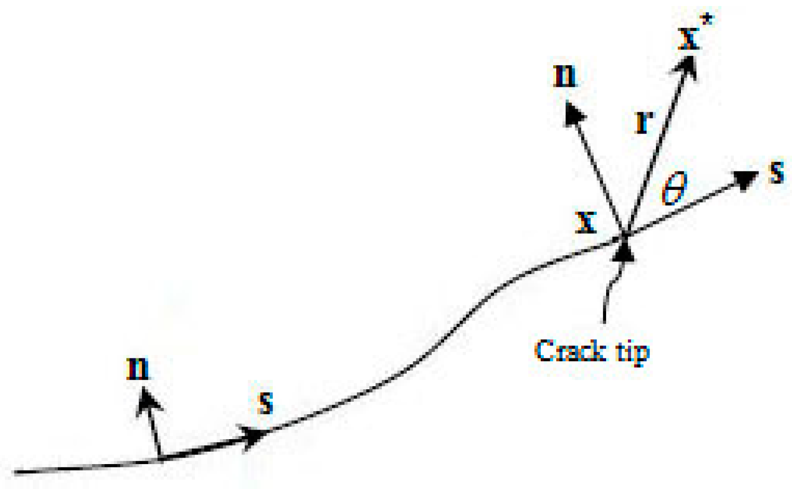
is a jump function used to characterize the displacement discontinuity within the crack-penetrating element:
where x is a Gauss point in the computational domain, x* is the closest point on the crack surface to x, and n is the unit-utward normal vector to the crack at x*.
is an additional function of the crack-tip element that reflects the singularity at the crack tip [12]:
where represent the local polar coordinates at the crack tip (as shown in Figure 1).
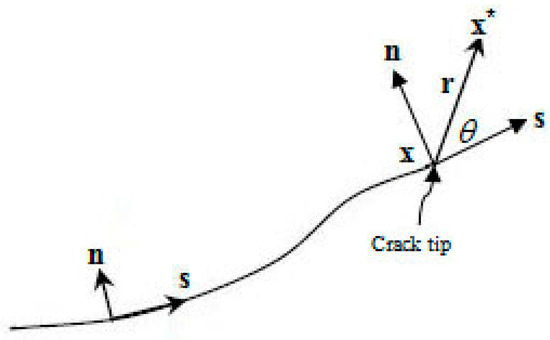
Figure 1.
Local polar coordinates.
For the elements containing cracks, the relative displacement of the same point on the crack surfaces can be obtained from Equation (1):
where represents the relative displacement of the same point on the crack surfaces.
2.2. Discrete Equations for Hydraulic Fracturing
After the displacement mode is constructed, the extended finite element governing equations for the hydraulic fracturing problem are derived through the principle of virtual work:
where is the water pressure on the crack surface ; is the external force on the boundary ; is the body force on the computational domain ; , , and are the Cauchy stress tensor, virtual displacement, and virtual strain, respectively.
Substituting the extended finite element approximate displacement expressions (1) and (4) into the extended finite element governing Equation (5), the discrete equations for hydraulic fracturing can be obtained:
The global stiffness matrix is formed by the assembly of the element stiffness matrices
the functional expressions of the strain matrices , , and can be found in Reference [13].
is the node displacement vector:
is the equivalent nodal load vector of the body force , the external force , and the water pressure , and it can be expressed as:
where l = 1, 2, 3, 4.
2.3. Contact Model
The extended finite element governing equations for the frictional contact problem can be obtained from the principle of virtual displacement as follows:
where represents the contact force vector acting on the crack surface within the global coordinate system.
It can be obtained from the governing Equation (11), Formula (5), and the discrete Equation (6):
where is the equivalent nodal load vector of the contact force vector on the crack surface.
The above formula can be written in the following form:
where , , and denote the relative displacements induced by the external load on the crack surface.
With
Equation (13) can be reformulated as follows:
where , , and are the global transformation matrices.
The above-mentioned formula represents the relationship between the relative displacements and forces on the contact surface.
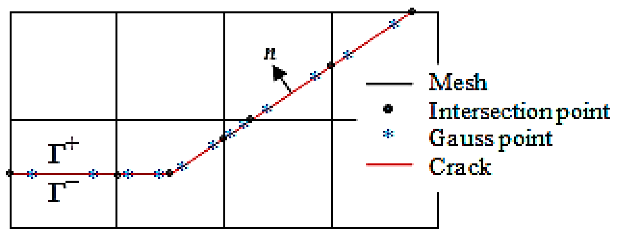
When addressing contact problems via the conventional finite element method, two conditions must be met. Firstly, the crack surface should align with the element boundary, and secondly, nodes must be present on the crack surface. In contrast, when employing the extended finite element method to tackle contact problems, the crack surface can traverse through the interior of the element, and there is no need for nodes on the crack surface. In this paper, the contact relationship on the crack surface is characterized by leveraging the relationship between the displacements and forces at the Gaussian points on the crack surface (as depicted in Figure 2).
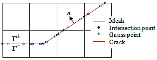
Figure 2.
Gaussian points on the crack surface.
The Gaussian points serve as contact point pairs. When considering the i-th contact point pair, it must adhere to both the geometric compatibility condition and the friction condition (as detailed in Reference [14]). These contact conditions can be formulated as the following non-smooth equations of the nonlinear complementary type:
where is the Coulomb friction coefficient.
It can be seen from Equation (15) that the vector is a function of the vector . Therefore, Equations (16) and (17) can be written as non-smooth equations of the nonlinear complementary type with as the variable:
The above formula is a non-smooth equation system model of the nonlinear complementary type for the plane friction contact problem. In this paper, the non-smooth damped Newton method proposed in Reference [14] is employed to directly resolve the aforementioned non-smooth equation system.
3. Stress Intensity Factor Calculation and Crack Propagation Criterion
3.1. Calculation of Stress Intensity Factor
The interaction integral method is employed to compute the stress intensity factor at the crack tip. The expression of the interaction integral is as follows:
where , , and are the displacement vector, stress tensor, and strain tensor, respectively; is the integral region around the crack tip; is the Kronecker delta; is the weight function; is the water pressure on the crack surface; the superscript 1 represents the real state and takes the numerical solution of the extended finite element method; and the superscript 2 represents the auxiliary state and takes the crack-tip asymptotic field.
is the interaction strain energy density of states 1 and 2, and its expression is as follows:
The stress intensity factor and the interaction integral are related as follows:
for plane strain, ; for plane stress, .
By choosing state 2 as the asymptotic fields of mode I and mode II, the stress-intensity factors of mode I and mode II corresponding to state 1 can be derived: , .
3.2. Crack Propagation Criterion
The maximum circumferential stress criterion is utilized as the crack propagation criterion to determine the crack propagation angle :
The equivalent stress intensity factor is calculated according to the following formula:
4. Numerical Examples
4.1. A Plate with a Single-Edge Crack
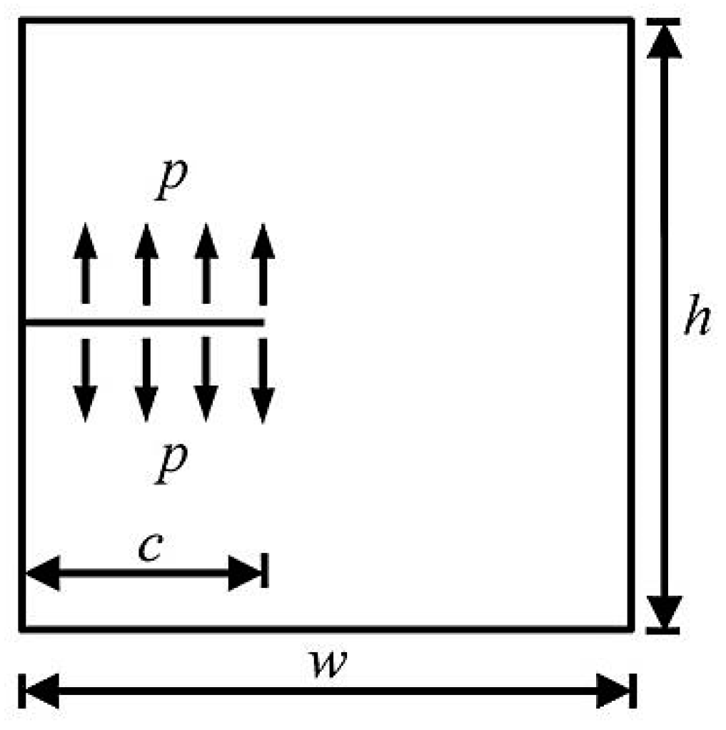
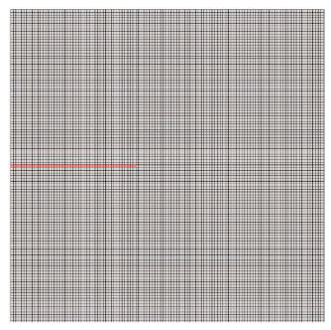
The rectangular plate with the length of a single-edge crack being is shown in Figure 3. The width of the flat plate is , the height is , and the uniformly distributed water pressure acts on the crack surface. The elastic modulus of the material of the rectangular plate is , and the Poisson’s ratio is . The finite element meshing is shown in Figure 4, the red line in the figure is crack.

Figure 3.
A rectangular plate with edge crack.
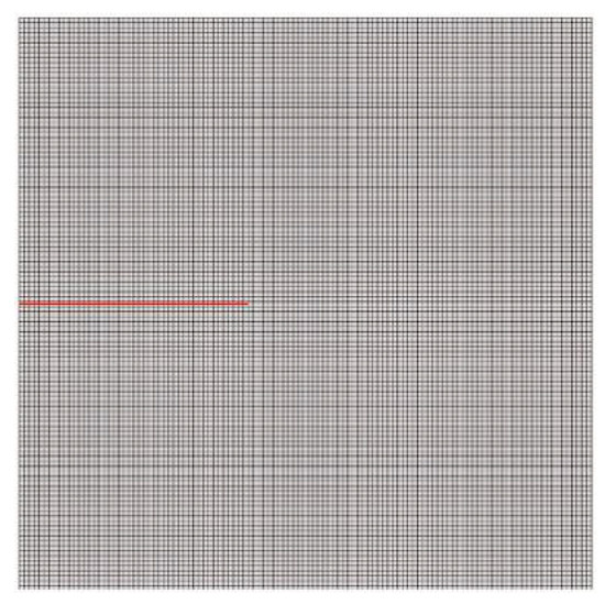
Figure 4.
Mesh generation.
Based on the superposition principle reported in Reference [15], the precise solution for the stress intensity factor under the action of uniformly distributed water pressure on the crack surface is as follow:
Define the normalized stress intensity factor
where is the stress intensity factor calculated by the method proposed in this paper. The normalized stress intensity factor for different elements are given in Table 1.

Table 1.
Normalized SIF values for different elements.
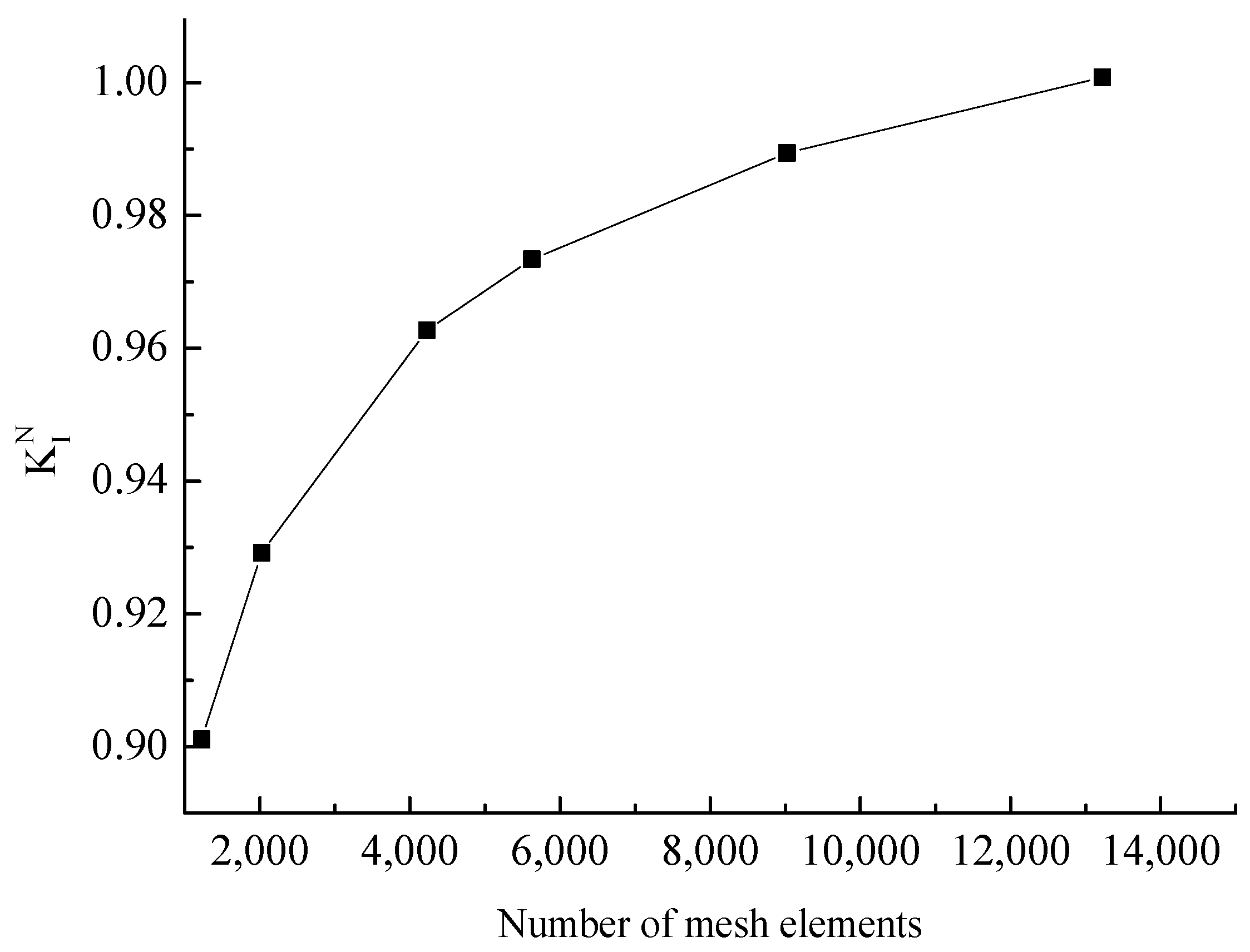
Figure 5 illustrates the impact of the quantity of mesh elements on the value of the normalized stress intensity factor. As can be observed from the figure, high computational precision can be attained even when the number of elements is comparatively small. As the number of elements increases, the computational error gradually decreases. When the number of mesh elements is around 10,000, the influence of the number of mesh elements on computational accuracy can be neglected.
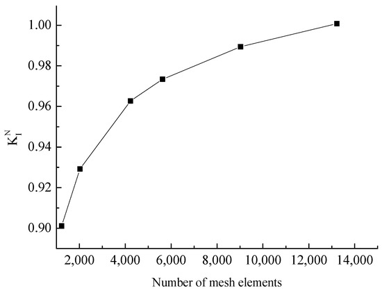
Figure 5.
The effect of mesh elements on normalized SIF.
Figure 6 presents the stress-intensity factors when the crack surface is subjected to different water pressures, with the number of mesh elements set at 13,225. From this figure, it is evident that the values of the stress-intensity factors computed by the method proposed in this paper are in good agreement with the exact solutions. This finding suggests that the method introduced in this paper can accurately calculate the stress-intensity factors under the action of uniformly distributed water pressures on the crack surface.
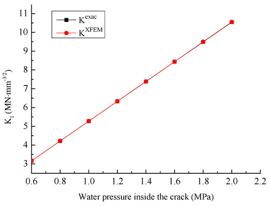
Figure 6.
The SIFs under different water pressures on the crack.
4.2. A Plate with a Through Crack
Figure 7 shows a rectangular plate with a through crack. The friction coefficient of the crack surface is , the bottom is under fixed constraints. Both the length and width of the flat plate are 10 m. Its top is subjected to the tangential uniformly distributed shear force and the normal uniformly distributed pressure . The elastic modulus is , and the Poisson’s ratio is .
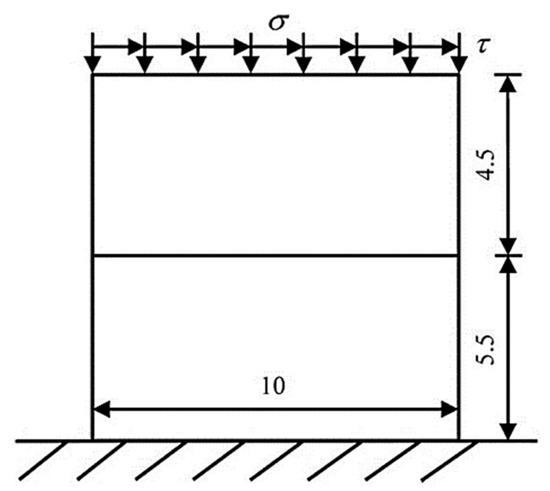
Figure 7.
Rectangular plate with through crack.
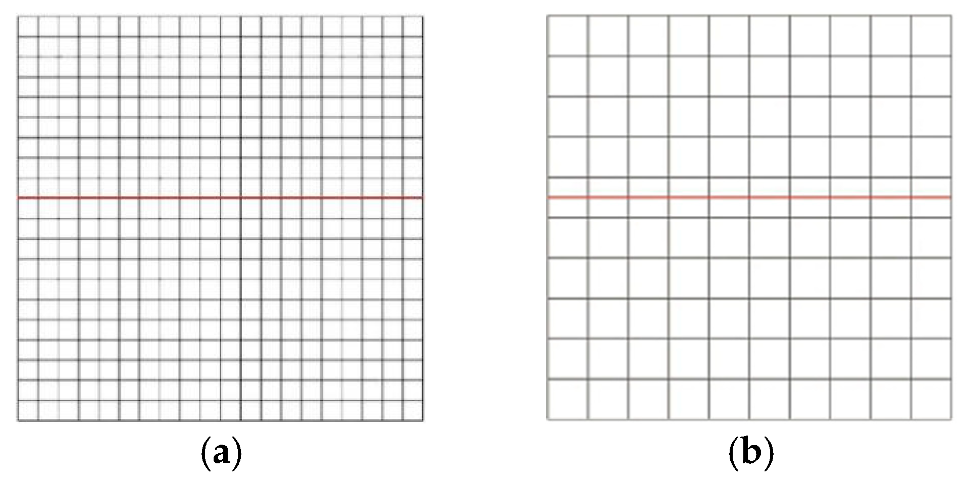
To validate the accuracy of the contact algorithm proposed in this paper, a comparison is made between this algorithm and the finite-element penalty function method. The finite-element mesh generation is illustrated in Figure 8a, where the computational model is partitioned into a total of 400 elements. Figure 8b shows the extended finite element mesh, which adopts four-node isoparametric elements. The computational model is divided into 100 elements in total. The red line in the Figure 8 is crack. The numerical example has undergone five iterations of calculation and met the convergence requirements, with a tolerance of 9.1104 × 10⁻⁹. Figure 9 shows the displacement contour plot. It can be seen from the figure that under the action of compressive-shear stress, the horizontal and vertical displacements of the upper and lower parts of the crack surface are continuous, indicating that the contact algorithm in this paper is effective. The stress contour plot is shown in Figure 10. As can be seen from the figure, the normal stress on the crack surface is continuous, while the tangential normal stress is discontinuous, which conforms to the conditions of the compressive stress contact surface.
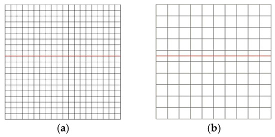
Figure 8.
Mesh generation. (a) Extended finite element mesh; (b) finite element mesh.
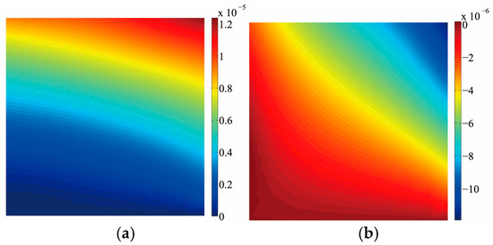
Figure 9.
Displacement contour (Unit: m). (a) Horizontal displacement; (b) vertical displacement.
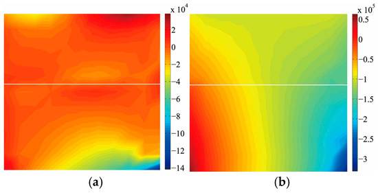
Figure 10.
Stress contour (Unit: Pa). (a) Normal stress ; (b) normal stress .
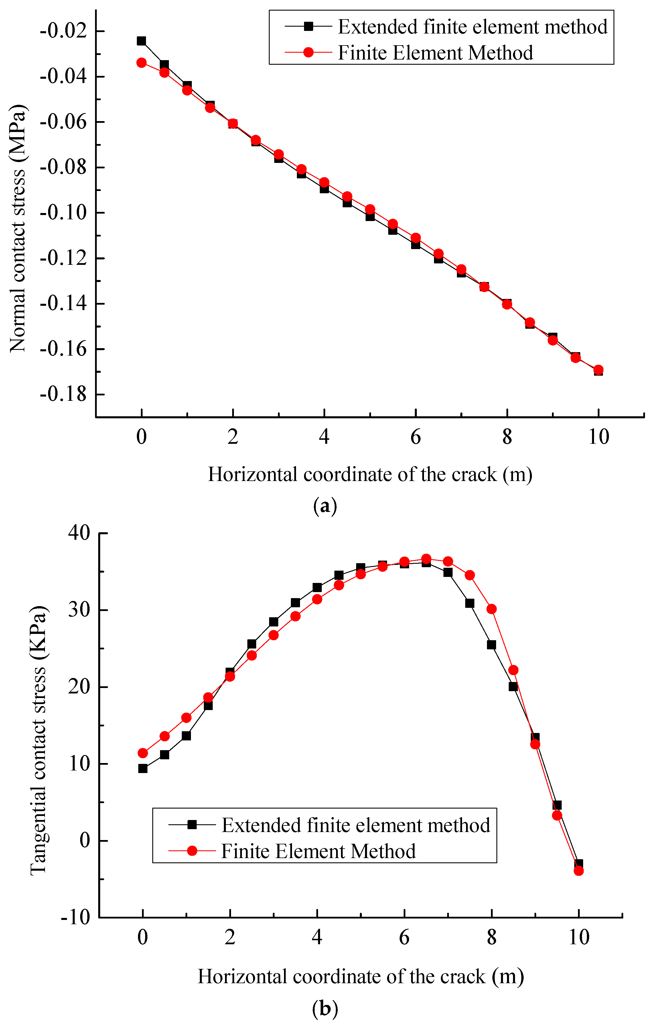
Figure 11 depicts the contact stresses on the crack surface computed by the finite-element penalty function method and the contact algorithm presented in this paper. From this figure, it is clear that the calculation results of the contact algorithm in this paper are in good agreement with those of the finite-element penalty function method, which implies that the contact algorithm in this paper is accurate. Table 2 showcases the normal contact forces, normal relative displacements, tangential contact forces, and tangential relative displacements of Gaussian points 1 to 20 on the crack surface.
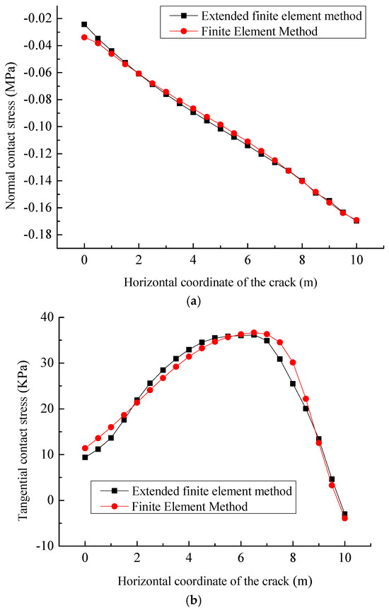
Figure 11.
Contact stresses on the crack surface. (a) Normal contact stress; (b) tangential contact stress.
Table 2.
Computational results of the slipping contact points 1–20.
4.3. A Plate with a Central Crack
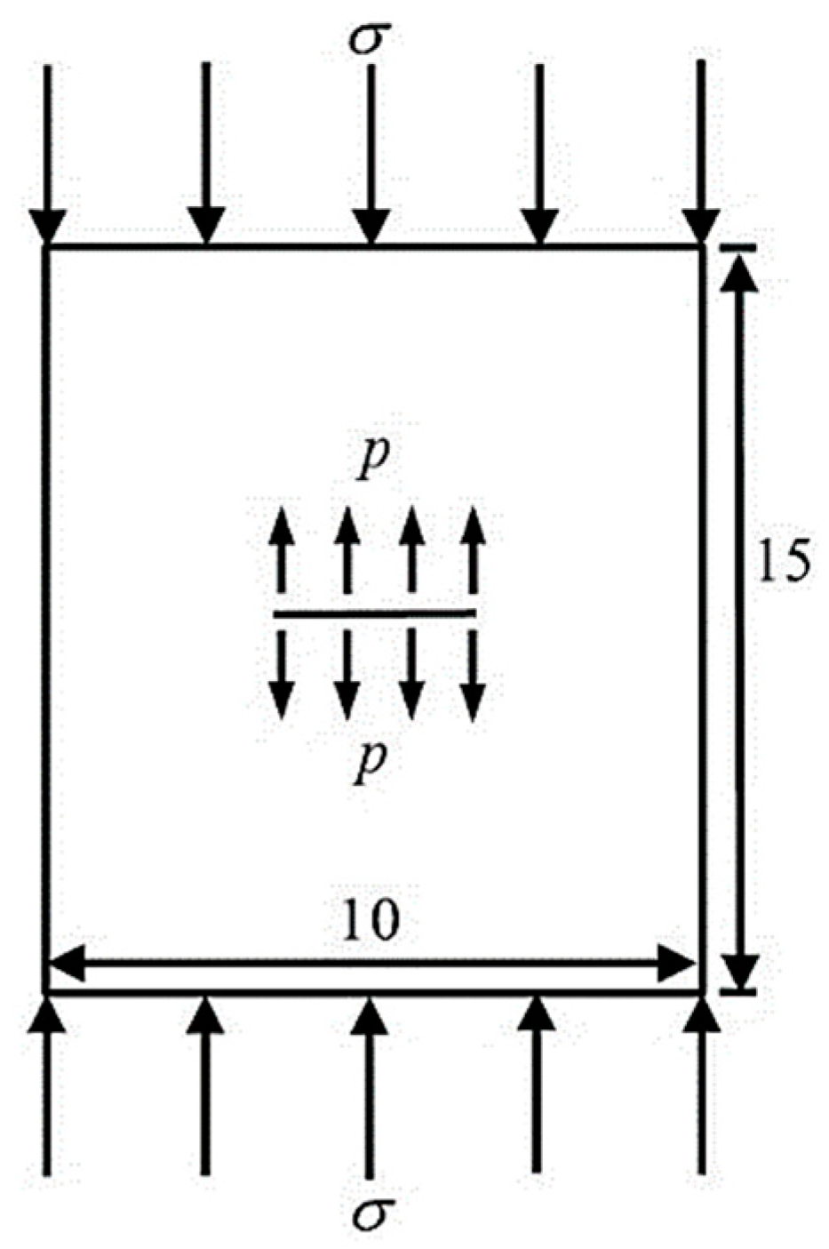
Figure 12 shows a rock specimen with a central crack. The length of the central crack is 2 m, the height of the specimen is 15 m, and the width is 10 m. The top of the specimen is subjected to an external axial pressure , and the crack surface is acted upon by a uniformly distributed water pressure . The elastic modulus of the rock specimen is , the Poisson’s ratio is , the fracture toughness is , and the friction coefficient of the crack surface is .
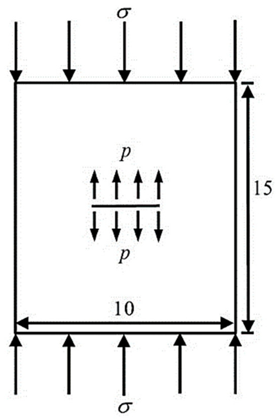
Figure 12.
Specimen with center crack.
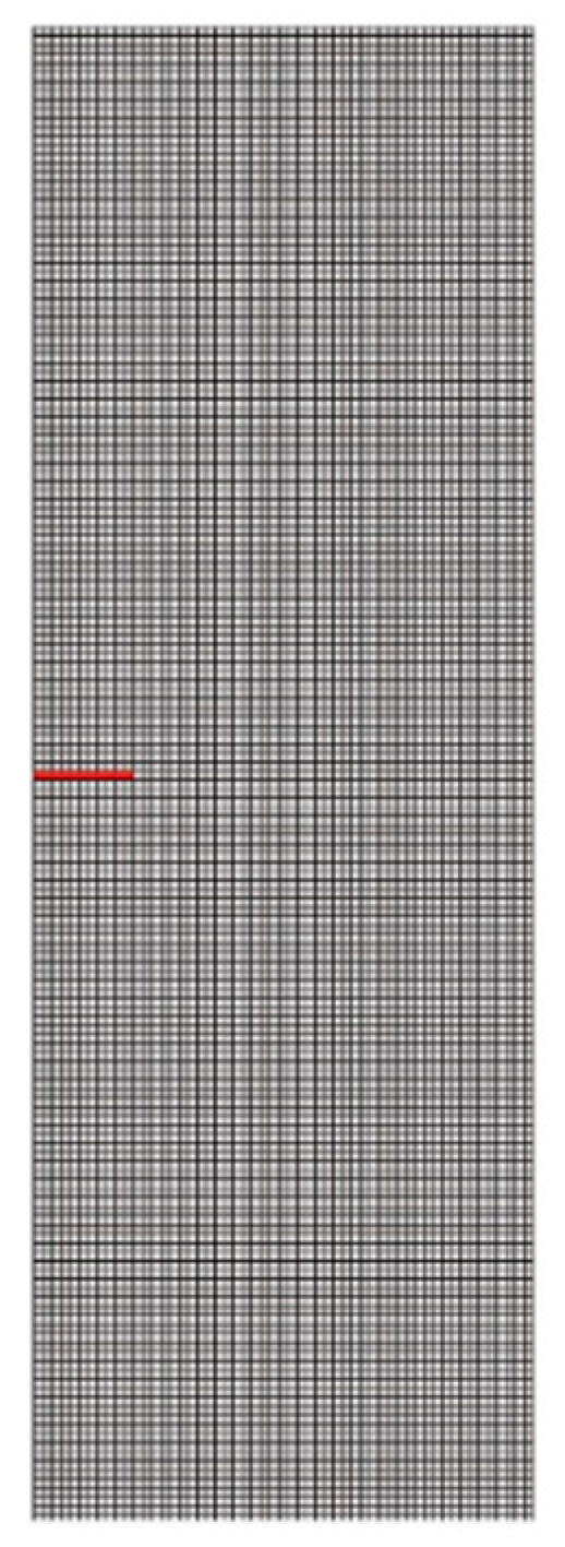
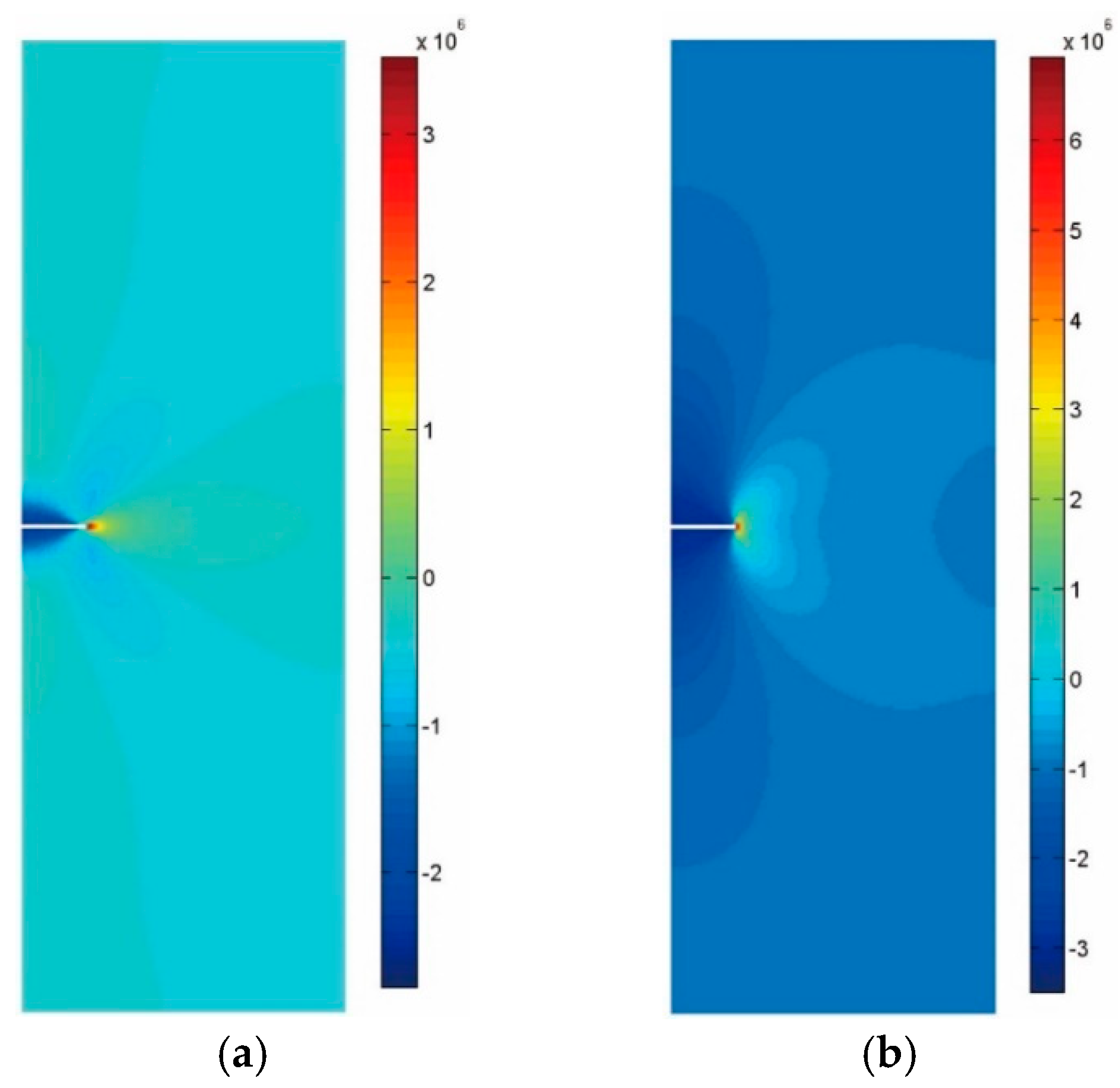
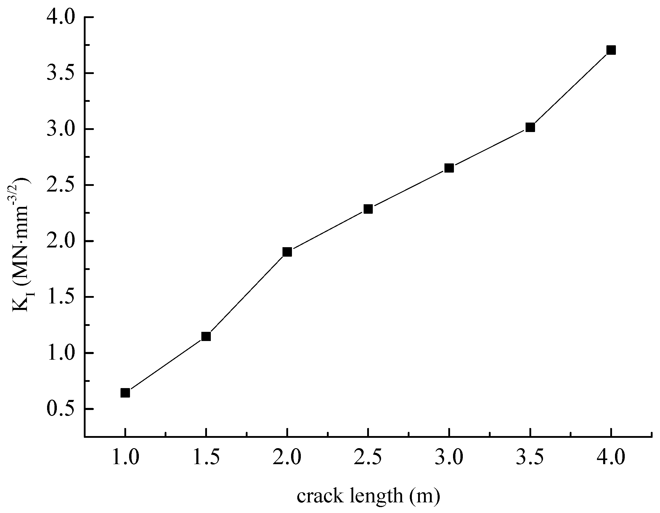
Considering the structural symmetry of the specimen, the right half of the specimen is taken. The mesh generation is shown in Figure 13, the red line in the figure is crack. The computational model is divided into 12,675 elements in total. The numerical example has undergone four iterations of calculation and met the convergence requirements, with a tolerance of 1.1586 × 10⁻¹⁰. Figure 14 shows the stress contour plot. It can be seen from the figure that under the combined action of the external axial pressure and the internal water pressure, an obvious stress concentration phenomenon appears at the crack tip of the rock specimen with a central crack. The stress-intensity factors under different crack lengths are shown in Figure 15, indicating that under the combined action of the external axial pressure and the internal water pressure, the stress intensity factor at the crack tip of the rock specimen increases as the crack length increases.
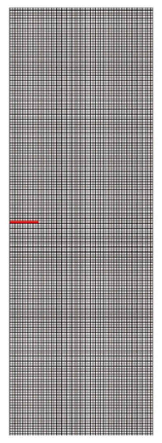
Figure 13.
Mesh generation.
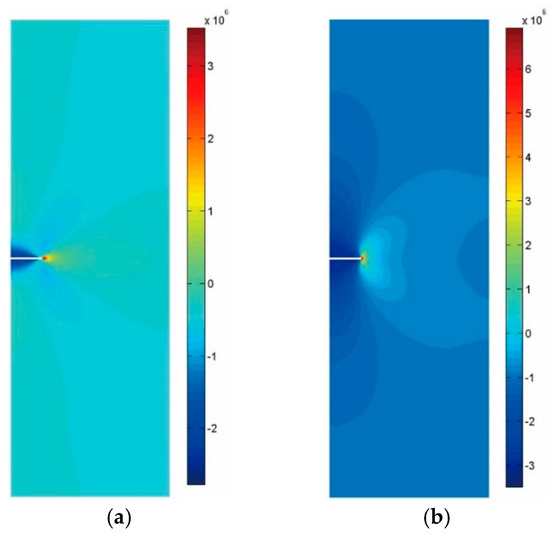
Figure 14.
Stress contour (Unit: Pa). (a) Normal stress ; (b) normal stress .

Figure 15.
The SIFs under different crack lengths.
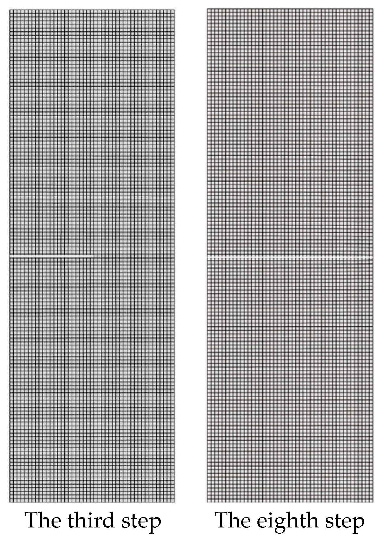
The water pressure within the crack commences at 0 MPa and steadily rises with an increment of 0.1 MPa. When the stress intensity factor at the crack tip surpasses the fracture toughness, the water pressure inside the crack at that moment is regarded as the critical water pressure. Figure 16 displays the crack propagation path under the influence of a critical water pressure of 3 MPa. The number of crack propagation steps amounts to eight, and the crack propagation step-length is set at 0.5 m. The crack propagation criterion employed is the maximum circumferential stress criterion. As can be discerned from the figure, the crack initiates propagation from the tip and extends in the horizontal direction. The numerical calculation results are in accordance with the experimental results reported in Reference [16].
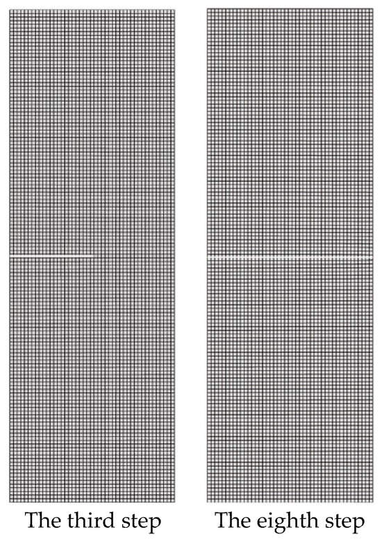
Figure 16.
The crack propagation path.
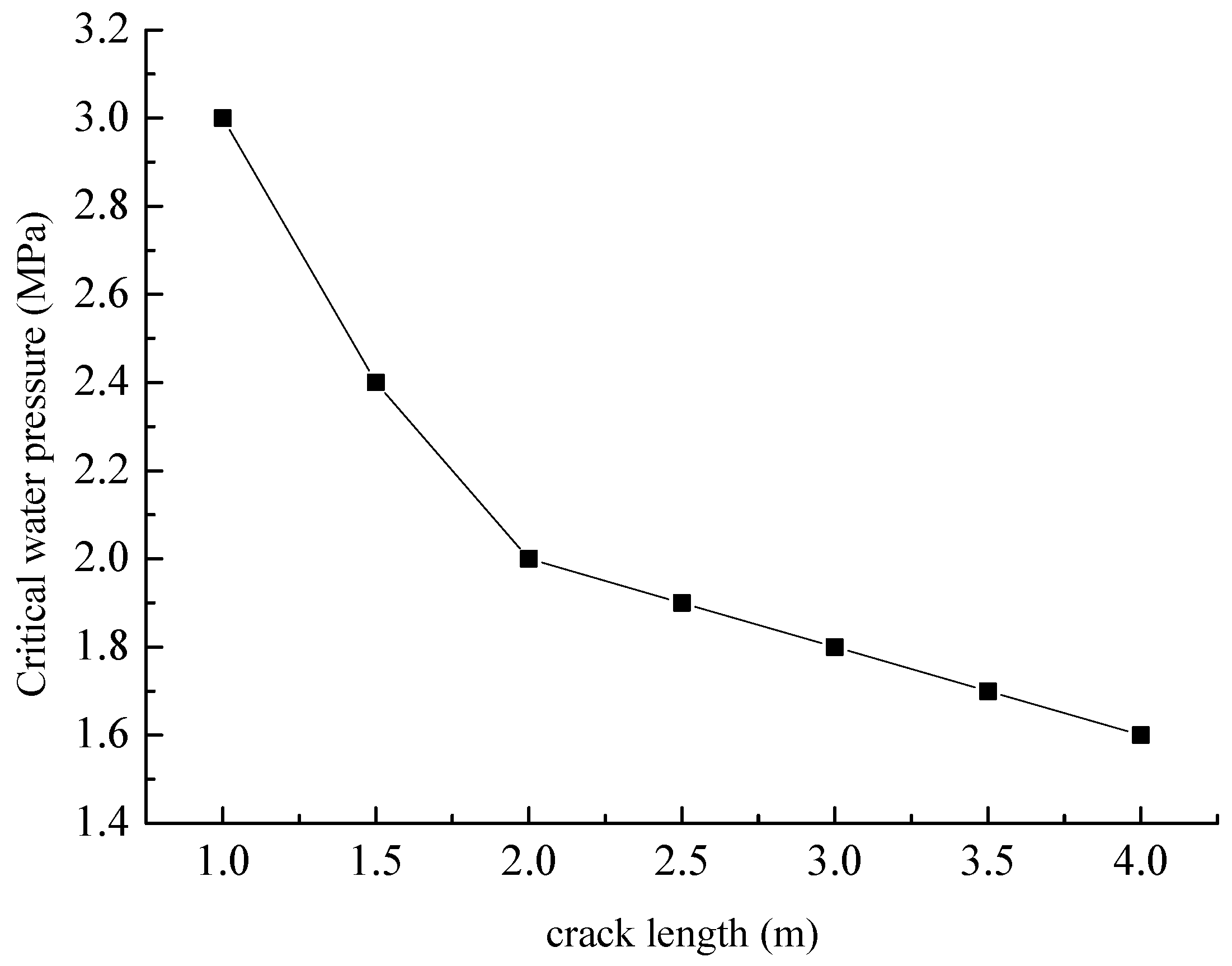
Figure 17 illustrates the critical water pressures corresponding to different crack lengths. From this figure, it is apparent that the critical water pressure declines as the crack length grows. Figure 18 presents the critical water pressures under varying external axial pressures. As can be observed from the figure, the critical water pressure rises in tandem with the increase in external axial pressure. The calculation outcomes are in agreement with the experimental findings reported in Reference [16]. The axial pressure exerts an inhibitory influence on crack initiation, leading to an increase in the critical water pressure.

Figure 17.
Critical internal water pressure under different crack lengths.
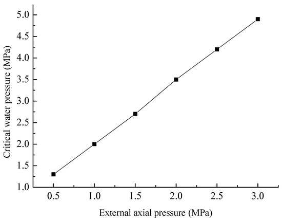
Figure 18.
Critical internal water pressure under different external axial pressures.
4.4. A Gravity Dam with an Initial Crack
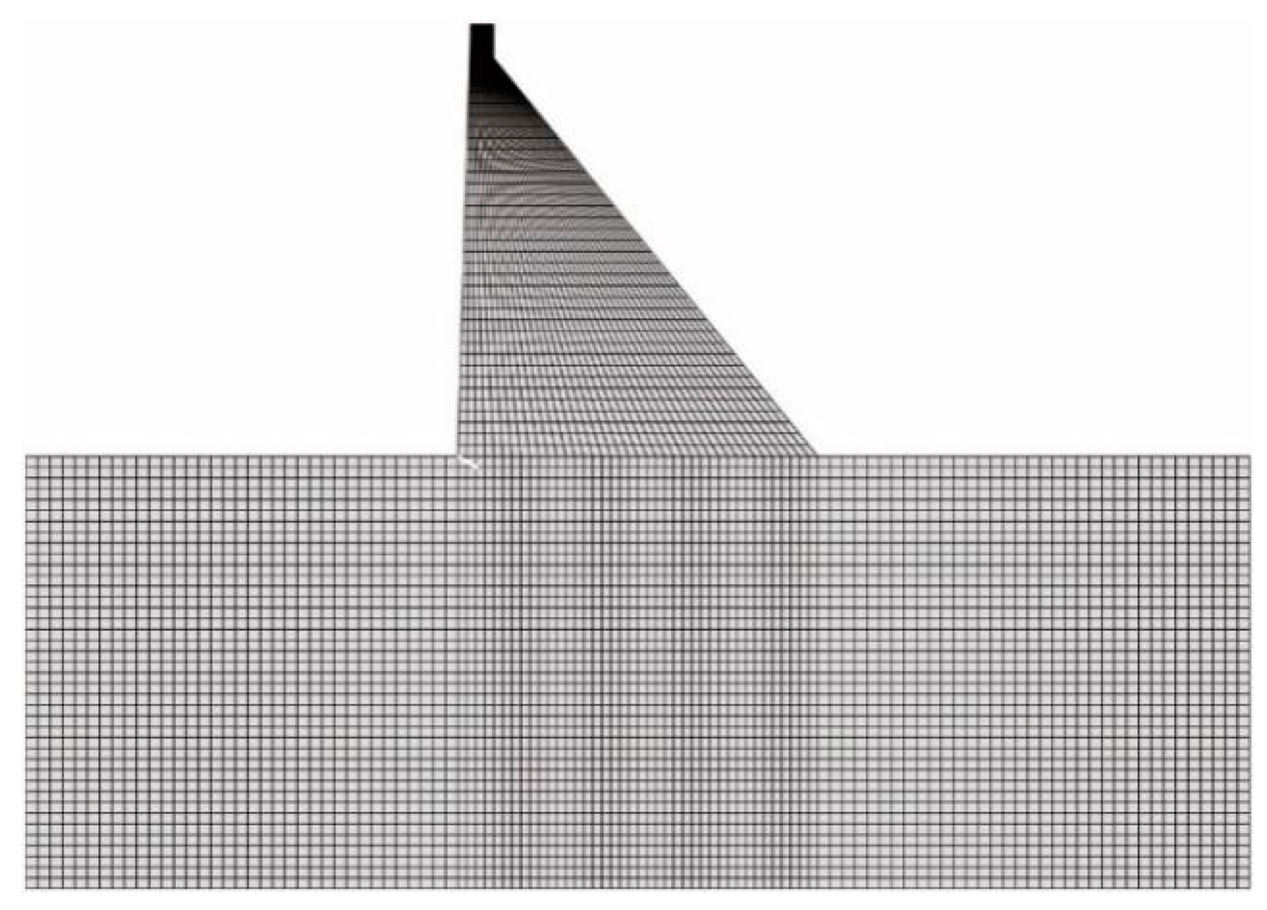
There is an initial crack with a length of 10 m at the foundation of a concrete gravity dam. The angle between this crack and the horizontal section of the dam heel is 30°. The height of the dam is 192 m, the width at the bottom of the dam is 159.8 m, and the width at the top of the dam is 10 m. The scope of the dam foundation extends 192 m upstream, downstream, and in the depth of the dam foundation, respectively, as shown in Figure 19. The upstream and downstream boundaries of the dam foundation are under normal constraints, and the bottom of the dam foundation is under fixed constraints. The computational parameters related to the materials of the gravity dam are shown in Table 3. The quadrilateral isoparametric elements are adopted for numerical analysis. The mesh generation is shown in Figure 20, with the number of elements being 5920 and the number of nodes being 6109.
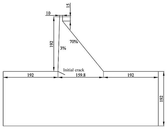
Figure 19.
Gravity dam with initial crack (unit: m).
Table 3.
Mechanical parameters of gravity dam materials.
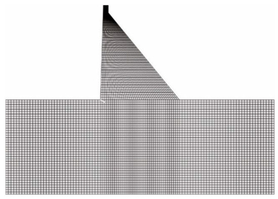
Figure 20.
Mesh division.
The main loads considered in the calculation include the self-weight of the dam, the upstream hydrostatic pressure, and the water pressure inside the crack. For the hydrostatic pressure, the method of gravity overload is adopted. Only the water gravity is increased while the water level remains at 192 m. The overload coefficient is the ratio before and after the increase in the water pressure. In this example, the overload coefficient is taken as 2.5.
The maximum circumferential stress criterion is adopted as the crack propagation criterion, and the crack propagation step length is taken as 3 m. There are a total of 12 crack propagation steps. Figure 21 shows the stress contour plot of the gravity dam obtained by the extended finite element calculation. It can be seen from the figure that stress concentration phenomena occur in both the dam heel and the crack tip areas, and the stress value in the dam heel area is significantly lower than that in the crack tip area.
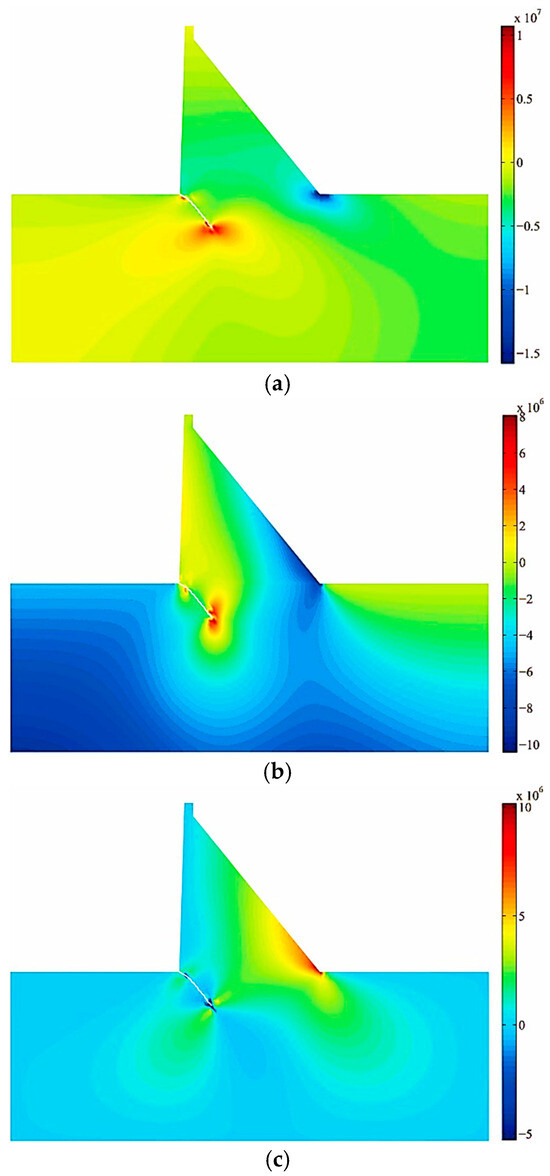
Figure 21.
Stress contour for gravity dam (Unit: Pa). (a) stress; (b) stress; (c) stress.
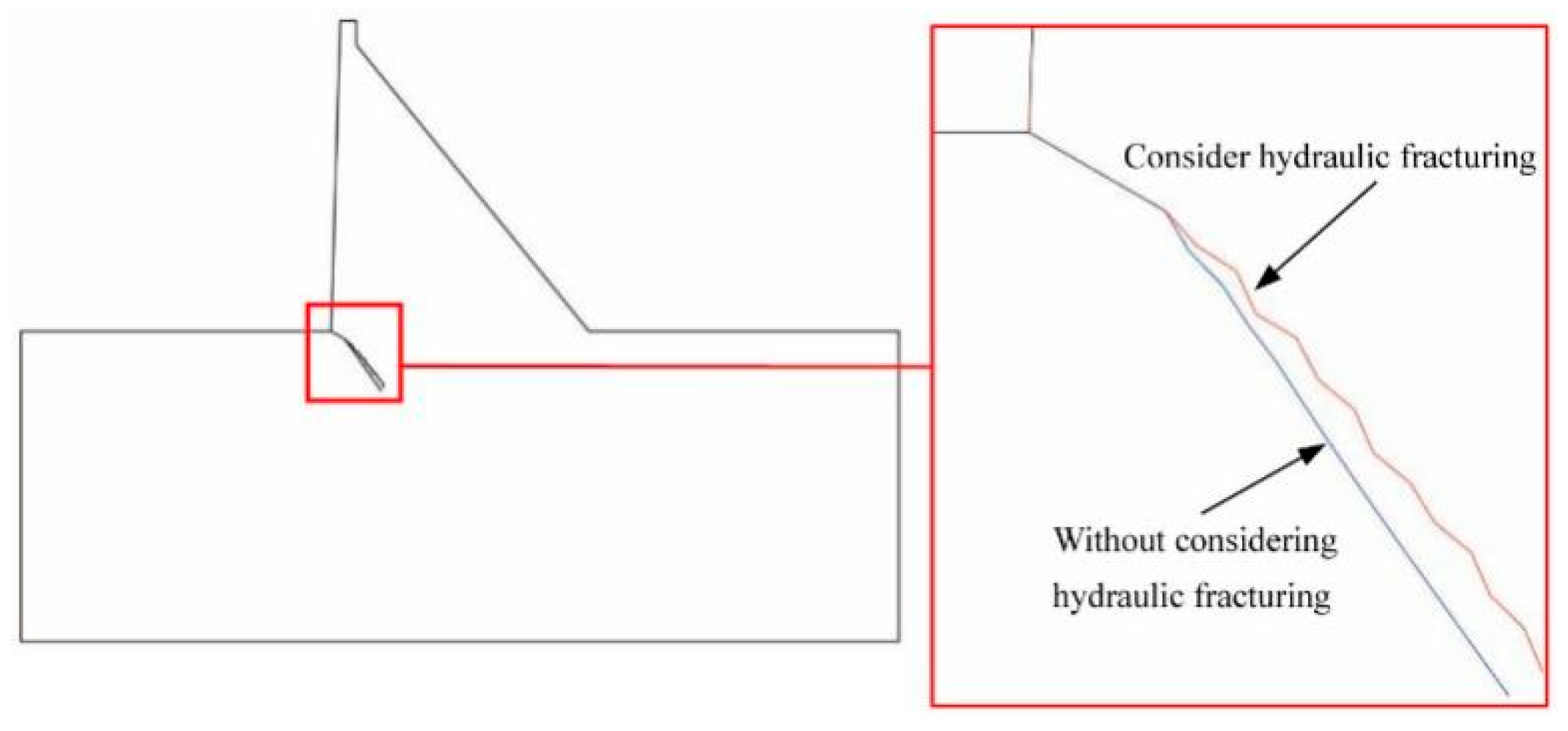
The crack propagation paths with and without considering hydraulic fracturing are shown in Figure 22. The crack propagation angle in the case of considering hydraulic fracturing is smaller than that in the case of not considering hydraulic fracturing.
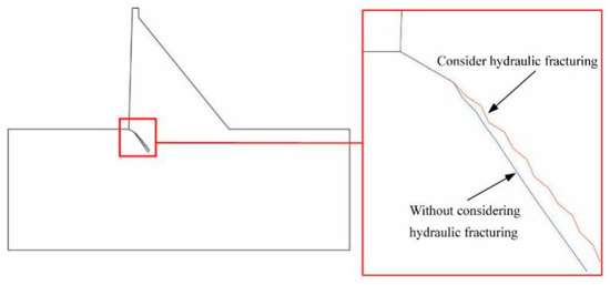
Figure 22.
Crack extension path of gravity dam.
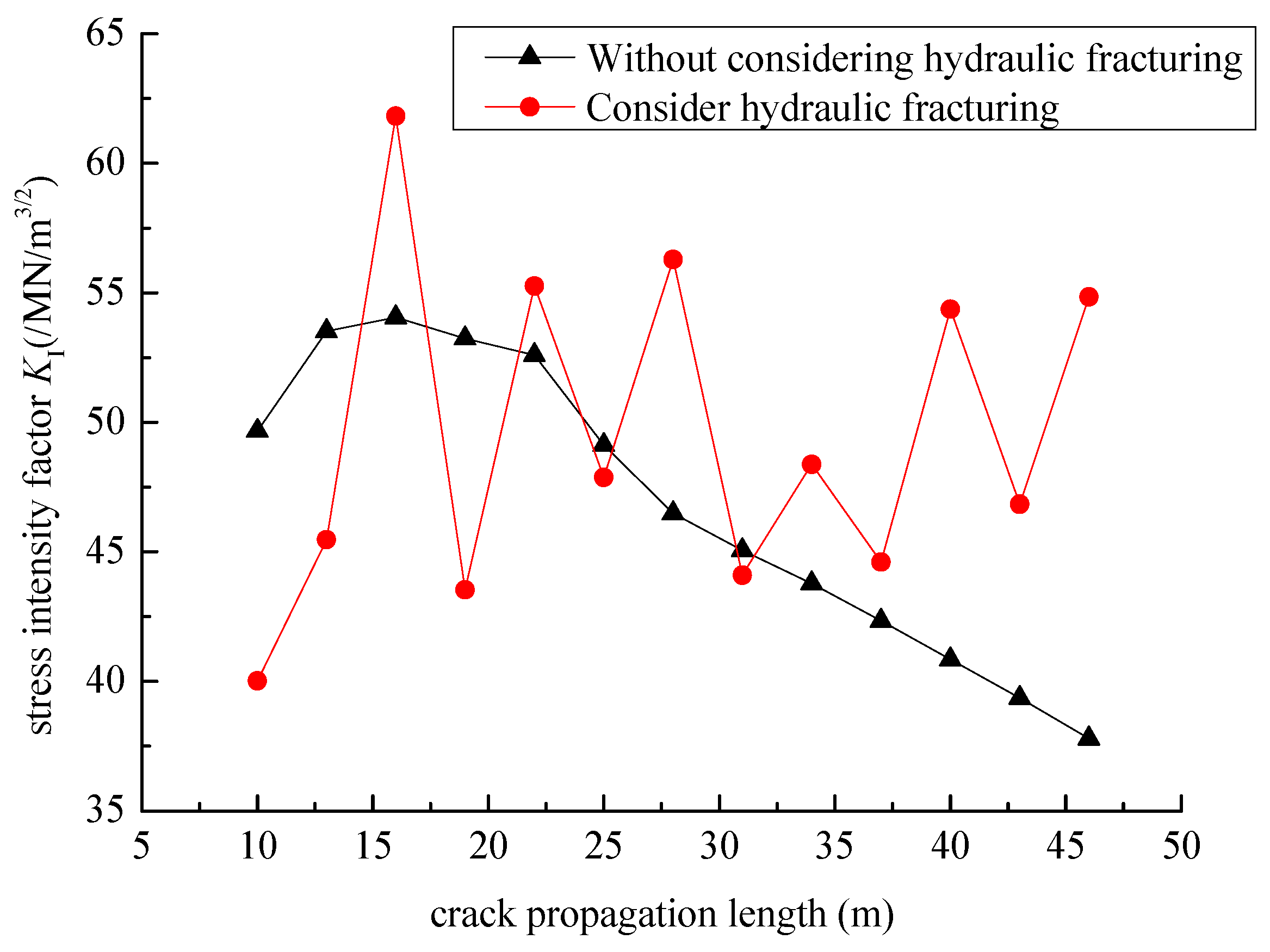
Figure 23 presents the relationship curve between the stress intensity factor and the crack length. When hydraulic fracturing is considered, the mode I stress-intensity factor fluctuates. Conversely, when crack hydraulic fracturing is not taken into account, the mode I stress-intensity factor remains relatively stable. As the crack propagates further, the mode I stress-intensity factor in the scenario where hydraulic fracturing is considered exceeds that in the scenario without considering it. This indicates that hydraulic fracturing can enhance the mode I stress-intensity factor at the crack tip. Consequently, the stability of the crack at the foundation of the gravity dam is diminished.
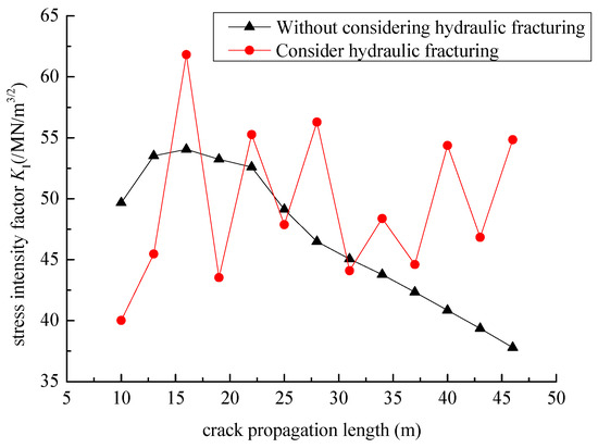
Figure 23.
Relationship curve between stress intensity factor and crack length.
5. Conclusions
This paper takes advantage of the extended finite element method in solving problems on moving discontinuous surfaces. By taking into account the virtual work principle of the water pressure distribution on the crack surface as well as the frictional contact of the crack surface, the governing equations for analyzing hydraulic fracturing and frictional contact problems via the extended finite element method are deduced. A numerical model based on the extended finite element method is developed to address the problems of hydraulic fracturing and frictional contact of rock cracks. The calculation model is applied to the hydraulic fracturing analysis of the specimens with central cracks and the gravity dams with initial cracks under the action of axial pressure. The following conclusions are obtained:
- (1)
- The values of the stress-intensity factors calculated by the method in this paper are consistent with the exact solutions, indicating that the method in this paper is accurate in calculating the stress-intensity factors when the crack surface is subjected to the action of uniformly distributed water pressures. Moreover, as the number of elements increases, the computational error gradually decreases.
- (2)
- The contact algorithm in this paper can effectively prevent the crack surfaces from interpenetrating. Its results are consistent with the calculation results of the finite-element penalty function method, indicating that the contact algorithm in this paper is accurate.
- (3)
- Under the combined action of the external axial pressure and the internal water pressure, the stress intensity factor at the crack tip of the rock specimen increases as the crack length increases. The critical water pressure decreases as the crack length increases; the critical water pressure increases as the external axial pressure increases. The axial pressure has an inhibitory effect on crack initiation, and the critical water pressure will increase.
- (4)
- Hydraulic fracturing will increase the mode I stress-intensity factor at the crack tip and reduce the stability of the cracks at the foundation of the gravity dam.
Author Contributions
Conceptualization, A.Z.; data curation, A.Z.; formal analysis, A.Z.; funding acquisition, A.Z.; software, A.Z.; writing—original draft preparation, A.Z.; writing—review and editing, A.Z. All authors have read and agreed to the published version of the manuscript.
Funding
This work was supported by the Joint Funds of the Zhejiang Provincial Natural Science Foundation of China under Grant No. LZJWY22E090008, the Nanxun Scholars Program of ZJWEU under Grant No. RC2023010814, and the National Natural Science Foundation of China under Grant No. 51279100.
Data Availability Statement
The original contributions presented in the study are included in the article, further inquiries can be directed to the corresponding author.
Conflicts of Interest
The authors declare no conflict of interest.
References
- Andree, G. Brittle Failure of Rock Materials Test Results and Constitutive Models; A. A. Balkema: Rotterdam, The Netherlands, 1995; pp. 1–5. [Google Scholar]
- Xu, Y.Q.; Zhan, D.Y. An Introduction to Rock Mass Hydraulics; Southwest Jiaotong University Press: Chengdu, China, 1995. [Google Scholar]
- Ahmad, D.; Parancheerivilakkathil, M.S.; Kumar, A.; Goswami, M.; Ajaj, R.M.; Patra, K.; Jawaid, M.; Volokh, K.; Zweiri, Y. Recent developments of polymer-based skins for morphing wing applications. Polym. Test. 2024, 135, 108463. [Google Scholar] [CrossRef]
- Qing, L.B.; Yu, K.L.; Xu, D.Q. Numerical analysis of macro-meso fractures in concrete gravity dams using extended finite element method. J. Hydroelectr. Eng. 2017, 36, 94–102. [Google Scholar]
- Shen, M.; Li, G.S. Extended finite element modeling of hydraulic fracture propagation. Eng. Mech. 2014, 31, 123–128. [Google Scholar]
- Shi, L.Y.; Li, J.; Xu, X.R.; Yu, T.T. Influence of hydraulic fracturing on natural fracture in rock mass. Rock Soil Mech. 2016, 37, 3003–3010. [Google Scholar]
- Zhang, J.N.; Yu, H.; Xu, W.L.; Lv, C.S.; Micheal, M.M.; Shi, F.; Wu, H.A. A hybrid numerical approach for hydraulic fracturing in a naturally fractured formation combining the XFEM and phase-field model. Eng. Fract. Mech. 2022, 271, 108621. [Google Scholar] [CrossRef]
- Lecampion, B. An extended finite element method for hydraulic fracture problems. Commun. Numer. Meth. Eng. 2009, 25, 121–133. [Google Scholar] [CrossRef]
- Shi, F.; Wang, D.B.; Li, H. An XFEM-based approach for 3D hydraulic fracturing simulation considering crack front segmentation. J. Pet. Sci. Eng. 2022, 214, 110518. [Google Scholar] [CrossRef]
- Zeng, Q.D.; Yao, J.; Shao, J.F. An extended fnite element solution for hydraulic fracturing with thermo-hydro-elastic–plastic coupling. Comput. Methods Appl. Mech. Engrg. 2020, 364, 112967. [Google Scholar] [CrossRef]
- Moës, N.; Dolbow, J.; Belytschko, T. A finite element method for crack growth without remeshing. Int. J. Numer. Methods Eng. 1999, 46, 131–150. [Google Scholar] [CrossRef]
- Fleming, M.; Chu, Y.A.; Moran, B.; Belytschko, T. Enriched element-free Galerkin methods for crack tip fields. Int. J. Numer. Methods Eng. 1997, 40, 1483–1504. [Google Scholar] [CrossRef]
- Zheng, A.X.; Luo, X.Q.; Chen, Z.H. Hydraulic fracturing coupling model of rock mass based on extended finite element method. Rock Soil Mech. 2019, 40, 799–808. [Google Scholar]
- Zheng, A.X.; Luo, X.Q. A mathematical programming approach for frictional contact problems with the extended finite element method. Arch. Appl. Mech. 2016, 86, 599–616. [Google Scholar] [CrossRef]
- Wang, J.; Shi, J.Q. Calculation of stress intensity factor for crack in a finite plate. Chin. J. Rock Mech. Eng. 2005, 24, 963–968. [Google Scholar]
- Xu, L.Q.; Tao, Y.C.; Liu, D.T. Hydraulic fracture test of rock-like materials under uniaxial compression. Adv. Sci. Technol. Water Resour. 2018, 38, 28–34. [Google Scholar]


Disclaimer/Publisher’s Note: The statements, opinions and data contained in all publications are solely those of the individual author(s) and contributor(s) and not of MDPI and/or the editor(s). MDPI and/or the editor(s) disclaim responsibility for any injury to people or property resulting from any ideas, methods, instructions or products referred to in the content. |
© 2025 by the author. Licensee MDPI, Basel, Switzerland. This article is an open access article distributed under the terms and conditions of the Creative Commons Attribution (CC BY) license (https://creativecommons.org/licenses/by/4.0/).