Improved Fruit Fly Algorithm to Solve No-Idle Permutation Flow Shop Scheduling Problem

Abstract

The no-idle permutation flow shop scheduling problem (NIPFSP), as a current hot topic, is widely present in practical production scenarios in industries such as aviation and electronics. However, existing methods may face challenges such as excessive computational time or insufficient solution quality when solving large-scale NIFSSP instances. In this paper, a discrete fruit fly optimization algorithm (DFFO) is proposed for solving the NIPFSP. DFFO consists of three phases, i.e., the smell search phase based on the variable neighborhood, the visual search phase based on the probabilistic model, and the local search phase. In the smell search phase, multiple perturbation operators are constructed to further expand the search range of the solution; in the visual search phase, a probabilistic model is constructed to generate a series of positional sequences using some elite groups, and the concept of shared sequences is adopted to generate new individuals based on the positional sequences and shared sequences. In the local search stage, the optimal individuals are refined with the help of an iterative greedy algorithm, so that the fruit flies are directed to more promising regions. Finally, the test results show that DFFO’s performance is at least 28.1% better than other algorithms, which verifies that DFFO is an efficient method to solve NIPFSP.

1. Introduction

Production scheduling plays a crucial role in achieving advanced manufacturing, and the modeling and optimization of production scheduling are important topics in the field of systems engineering. This paper investigates the no-idle permutation flow shop scheduling problem (NIPFSP), which is an extension of the classical permutation flow shop scheduling problem. In NIPFSP, each machine must operate continuously from the beginning until the completion of the final job without any interruption [1]. The application areas of NIPFSP include casting production and fiberglass processing, among others [2,3].

Implementing no-idle shop scheduling can effectively reduce idle energy consumption of machine tools, making it an effective approach for energy conservation and emission reduction in the machining industry. Given the engineering and academic significance of NIPFSP, researchers at home and abroad have conducted a series of studies on this topic. Yin et al. [4] addressed NIPFSP with the objective of minimizing makespan by employing the fruit fly optimization algorithm as the main framework and incorporating the immune algorithm’s stimulation mechanism to enhance the algorithm’s search capabilities. Yan et al. [5], inspired by the concepts of variable neighborhood search and iterative greedy algorithms, proposed a new hybrid bird swarm algorithm to minimize the maximum completion time for NIPFSP. Experimental tests demonstrated the effectiveness of the algorithm. Zhao et al. [6] investigated NIPFSP with the objective of minimizing total tardiness under release time constraints. They designed an iterative greedy algorithm to solve the problem, and extensive experiments validated the improved algorithm’s effectiveness. Zhao et al. [7] studied a multi-objective hybrid NIPFSP with the objectives of minimizing maximum completion time and minimizing maximum tardiness. They proposed a multi-objective discrete sine optimization algorithm. Pei et al. [8], targeting NIPFSP with the goal of minimizing total tardiness, proposed a hybrid evolutionary algorithm based on the critical block structure.

The fruit fly optimization algorithm (FFO), proposed by Pan [9] based on the foraging behavior of fruit flies, is an evolutionary algorithm. Wang et al. [10] compared the FFO with more than ten metaheuristic algorithms, including artificial bee colony, ant colony optimization, and fish swarm algorithms, using benchmark instances. The results verified the strong optimization capability of FFO, attracting widespread attention. FFO has been widely utilized across multiple domains, including electric load prediction and parameter estimation. Ibrahim et al. [11] implemented a wind-driven FFO for identifying parameters in photovoltaic cell models. Similarly, Saminathan and Thangavel [12], along with their team, integrated the whale algorithm with FFO to tackle energy-saving challenges involving delays. Hu et al. [13] applied a combination of FFO and deep reinforcement learning to forecast energy usage in datasets from three extensive pipelines in China. In recent years, the straightforward design of FOA, and its parallel search framework, has facilitated its integration with various problem-specific search mechanisms, driving its redevelopment and achieving significant results in addressing production scheduling problems. Zhu et al. [14] proposed a discrete knowledge-guided learning FFO to address no-wait distributed flow shop scheduling problems. Guo et al. [15] designed an FFO based on a differential flight strategy to solve distributed flow shop scheduling problems with sequence-dependent setup times. Furthermore, Guo et al. [16] introduced an FFO to minimize the total flow time in distributed flow shop scheduling problems. This algorithm employed an initialization method that considered both population quality and diversity, and its effectiveness was validated through experimental testing.

In summary, metaheuristic algorithms possess general applicability, making them suitable for various optimization problems. However, this generality also introduces certain limitations, as they often overlook the unique structures and characteristics of specific problems. For flow shop scheduling problems, such algorithms frequently fail to design operators tailored to problem-specific features, such as job processing sequences. Consequently, their search efficiency and solution quality may be suboptimal. This paper proposes a discrete fruit fly optimization algorithm (DFFO) to solve the NIPFSP with the objective of minimizing makespan. The main contributions of this paper are as follows.

(1)

Using the characteristics of specific problems, multiple perturbation operators are designed to enhance the global search ability of the algorithm.

(2)

A probabilistic model based on elite subsets is constructed, and the concept of common sequence is introduced. The evolution of fruit flies is achieved through location sequences and common sequences.

(3)

The iterative greedy algorithm is used to conduct local searches for the best individuals and guide the fruit fly population to move to a more promising area.

(4)

Finally, the experiment verifies that DFFO is an effective method to solve NIPFSP.

The rest of this article is organized as follows. The objectives and constraints of the NIPFSP are set out in Section 2. Section 3 describes the specific steps that DFFO takes to address NIPFSP. Section 4 presents numerical analysis and comparison. Section 5 summarizes this paper and provides prospects for further research.

2. Problem Description

The NIPFSP can be described as follows [5]: A set of $n$ jobs $J=\{J_1,J_2,\dots ,J_n\}$ needs to be processed on $m$ machines $M=\{M_1,M_2,\dots ,M_m\}$ following the same routing sequence. Each job consists of m operations, and the i-th operation can only be performed on machine M_i. Notably, there must be no idle time between two consecutive jobs on the same machine. Once an operation starts, it cannot be interrupted midway, and each machine can process at most one job at a time. This study aims to minimize the maximum completion time (makespan) $C_{\max }$. The meanings of the symbols used in this paper are shown in

Table 1. Meaning of symbols.

Symbol	Implication
i	$\mathrm{Machine} \mathrm{index}, i\in \{1,2,\dots k\dots ,m-1\}$
j	$\mathrm{Job} \mathrm{index}, j\in \{1,2,\dots ,n\}$
$\pi =[\pi (1),\pi (2),\dots ,\pi (n)]$	Represents a complete job ordering
${\pi }^q(j)$	Represents a partial sequence of $\pi$
$G({\pi }^q(j),k.k+1)$	Represents the difference in completion times between machines k and k + 1 after completing sequence ${\pi }^q(j)$
$P(\pi (j),k)$	Denotes the processing time of job $\pi (j)$ on machine k
$C_{\max }$	The makespan

.

The maximum completion time $C_{\max }$ is calculated as follows:

$$\begin{array}{l}G({\pi }^q(1),k,k+1)=P(\pi (1),k+1),\\ k=1,2,\dots ,m-1\end{array}$$

(1)

$$\begin{array}{l}G({\pi }^q(j),k,k+1)=\max \{G({\pi }^q(j-1),k,k+1)\\ -P(\pi (j),k\}+P(\pi (j),k+1)\\ j=2,3,\dots ,n,k=1,2,\dots ,m-1\end{array}$$

(2)

$$\begin{array}{l}{C}_{\max }=\\ {\displaystyle \sum _{k=1}^{m-1}G({\pi }^q(n),k,k+1)+{\displaystyle \sum _{j=1}^{n}P(\pi (j),1)}}\end{array}$$

(3)

Equation (1) is the difference between the time to complete the first job on machine k and machine k + 1. Equation (2) is the difference in time between the completion of job ${\pi }^q(j)$ on machine k and machine k + 1. Equation (3) is the makespan of NIPFSP.

3. DFFO Algorithm

This section provides a detailed description of the DFFO, which comprises four main phases: population initialization, smell search based on variable neighborhood search, visual search using a probability model, and a local search phase to refine the current best solution. Figure 1 presents the flowchart of the DFFO algorithm.

3.1. Population Initialization

This paper adopts a job sequence-based encoding method, where each fruit fly represents a complete job sequence, and a feasible solution $\pi =\{\pi (1),\pi (2),\dots ,\pi (n)\}$ corresponds to a scheduling plan. A high-quality initial population can facilitate rapid optimization in subsequent sub-populations, thereby improving the algorithm’s performance. The NEH (Nawaz–Enscore–Ham) heuristic [17] is a widely used method for obtaining good solutions quickly. Therefore, this paper combines two initialization strategies: 50% of the individuals are generated using the NEH heuristic, and the other 50% are generated using a random initialization approach.

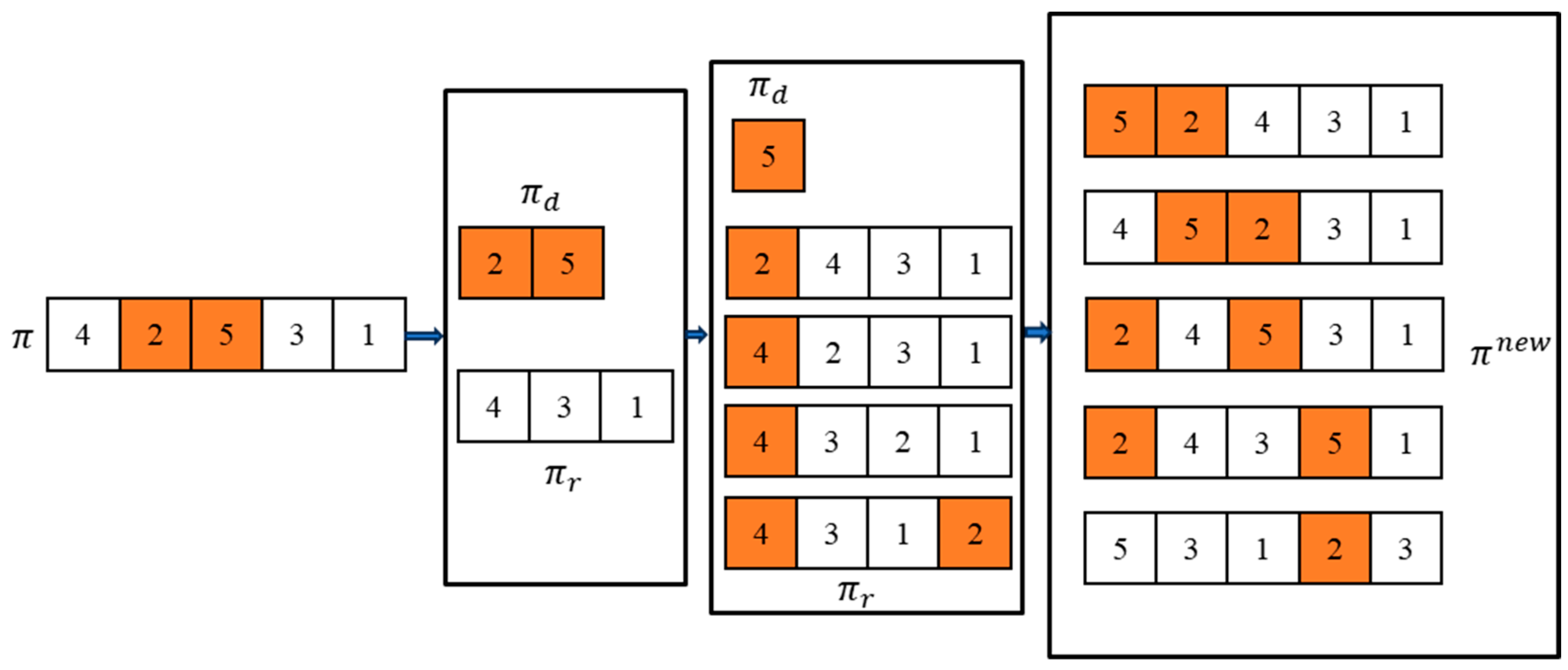
3.2. Smell Search Phase Based on Variable Neighborhoods

The smell search phase represents the evolutionary phase of fruit flies. According to the literature [18], no single neighborhood structure is universally applicable to solve all problems. In the DFFO algorithm, a set of neighborhood structures is specifically designed based on the unique characteristics of NIPFSP. This neighborhood structure set is used to develop various local search operators, including swap, double swap, bundle insertion, and reverse-block insertion. The neighborhood structures are described as follows:

S₁ (swap): randomly swaps the positions of two different jobs.

S₂ (double swap): performs two consecutive swap operations.

S₃ (bundle insertion): randomly removes two jobs from the solution and inserts them as a bundle into all possible positions in the remaining sequence.

S₄ (insert-reverse block insertion): randomly selects multiple jobs from the solution, bundles them, shuffles their order, and inserts them into all possible positions in the remaining sequence.

The DFFO algorithm employs a variable neighborhood descent (VND) strategy [5] to explore potential search regions. Each individual sequentially applies S₁ through S₄. If a neighborhood solution improves upon the previous solution, it replaces the latter. To illustrate the process clearly, a detailed example is presented in Figure 2.

3.3. Visual Search Phase Based on a Probability Model

In traditional FFO algorithms, there is only a single central fruit fly, and all fruit flies fly towards it during the visual search phase. However, this approach provides limited information and may lead to suboptimal algorithm performance [16]. To address this, this study extends the single central fruit fly to multiple elite individuals. By collecting feature information from these elite fruit flies, a probability model is established. Fruit flies evolve by continuously learning from the probability model. In summary, this paper proposes a visual search phase based on a probability model, as described by Equation (4).

$${\pi }_{new}={\pi }_{old}\otimes \{R(p\circ {\pi }_{center})\leftarrow {\pi }_{com}\}$$

(4)

where ${\pi }_{new}, {\pi }_{old}$ represents the new solution and the old solution before and after the update, respectively. ${\pi }_{com}$ is the common sequence shared by the average elite individuals. $\otimes$ denotes the crossover operation. $R(p\circ {\pi }_{center})$ is the position of all jobs generated using the probability model. $R(p\circ {\pi }_{center})\leftarrow {\pi }_{com}$ refers to the new sequence obtained by inserting the positions generated by $R(p\circ {\pi }_{center})$ into ${\pi }_{com}$. The crossover method employs partial matching crossover (PMX). The detailed steps of the visual search phase based on the probability model are as follows:

(1) Construction of the probability model. The current population is sorted based on fitness values, and the top $\lambda \times PS$ individuals are selected to form the elite population, where the population size is PS. $\lambda \in (0,1)$ is used to control the size of the elite population. Based on the elite population, a probability model is constructed. Let $P(t)$ denote the probability matrix for the t-th generation, and $p_{i,j}$ represents the probability of job i appearing in position j. The calculation of $p_{i,j}$ is as follows:

$$\begin{array}{l}{p}_{i,j}(t)=(1-\alpha )[(1-\beta )p_{i,j}(t-1)\\ +{\displaystyle \frac{\beta }{j\times PS\times \lambda }}{\displaystyle \sum _{k=1}^{PS\times \lambda }{I}_{i,j}^k}]+{\displaystyle \frac{\alpha }{j}}{I}_{i,j}^{best}\end{array}$$

(5)

$$I_{i,j}^k=\left\{\begin{array}{ll}1\hfill & The i\text{-}th job in k appears at or before position j \hfill \\ 0\hfill & \mathit{else}\hfill \end{array}\right.$$

(6)

$$I_{i,j}^{\mathit{best}}=\left\{\begin{array}{ll}1\hfill & The i\text{-}th job in the optimal entity appears at or before position j\hfill \\ 0\hfill & \mathit{else}\hfill \end{array}\right.$$

(7)

where $p_{i,j}(0)={\displaystyle \frac{1}{n}}$, $I_{\mathrm{i},\mathrm{j}}^k,I_{i,j}^{best}$ are the indicator functions for the k-th individual and the optimal individual in the fruit fly population, respectively. $\alpha ,\beta \in (0,1)$ represents a parameter, and $\alpha =\beta =0.1$. The optimal individual is the smallest makespan in the group.

(2) Calculation of the common sequence. The common sequence reflects the frequency with which a job appears in a specific position. Based on this concept, the DFFO algorithm introduces the idea of a common sequence, facilitating the evolution of fruit flies through interactions between position sequences and the common sequence. In this phase, the Borda method is employed to calculate the total score (votes) for each job appearing in each position within the common sequence. Jobs are then sequentially assigned to positions based on their scores. If multiple jobs have the same score, one is randomly selected from those with equal scores to be placed in that position.

(3) Model sampling. Reference [19] proposed the following sampling method: Use the roulette wheel method to select a job i and place it in position j in the sequence. Normalize the probability matrix P. Repeat the above process until a complete sequence is generated. However, during the normalization of the probability matrix P, the entire matrix needs to be traversed continuously, resulting in high time complexity. To address this, this study adopts a job-centric approach. The roulette wheel method is applied to select the position of each job in the common sequence. Then, based on the generated position information, all jobs are inserted into a new sequence.

First, for each job in ${\pi }_{com}$, generate a random number r between 0 and 1. Assign the position with the smallest probability greater than r as the current job’s position. Let $Rp$ represent the generated position sequence, and $\pi$ denote the newly generated sequence. For each job ${\pi }_{com}(i)$ in ${\pi }_{com}$, if $\pi (Rp(i))$ does not contain the job, perform $\pi (Rp(i))={\pi }_{com}(i)$. Otherwise, find the nearest vacant position after $Rp(i)$ and insert ${\pi }_{com}(i)$ into that position. If no vacant position exists after $Rp(i)$, find the nearest vacant position before $Rp(i)$ and insert.

To provide a detailed example illustrating the above process, assume the population consists of five fruit flies: $[4,3,1,0,2]$, $[0,3,4,2,1]$, $[1,2,4,3,0]$, $[1,0,4,3,2]$, and $[4,0,2,1,3]$, where $[4,3,1,0,2]$, $[0,3,4,2,1]$, and $[1,2,4,3,0]$ are elite individuals, and $[4,3,1,0,2]$ is the best individual.

First, calculate the probability model P.

① Initialize P and calculate I and I^best.

$$\begin{gathered} P(0)=\left(\begin{array}{ccccc}0.2& 0.2& 0.2& 0.2& 0.2\\ 0.2& 0.2& 0.2& 0.2& 0.2\\ 0.2& 0.2& 0.2& 0.2& 0.2\\ 0.2& 0.2& 0.2& 0.2& 0.2\\ 0.2& 0.2& 0.2& 0.2& 0.2\end{array}\right) \\ I=\left(\begin{array}{ccccc}1& 1& 1& 2& 3\\ 1& 1& 2& 2& 3\\ 0& 1& 2& 2& 3\\ 0& 2& 2& 3& 3\\ 1& 1& 2& 3& 3\end{array}\right) \\ {I}^{best}=\left(\begin{array}{ccccc}0& 0& 0& 1& 1\\ 0& 0& 1& 1& 1\\ 0& 0& 0& 0& 1\\ 0& 1& 1& 1& 1\\ 1& 1& 1& 1& 1\end{array}\right) \end{gathered}$$

② Calculate P

$$P=\left(\begin{array}{ccccc}0.192& 0.177& 0.172& 0.202& 0.2\\ 0.192& 0.177& 0.215& 0.202& 0.2\\ 0.162& 0.177& 0.182& 0.177& 0.2\\ 0.162& 0.242& 0.215& 0.210& 0.2\\ 0.162& 0.227& 0.215& 0.210& 0.2\end{array}\right)$$

Normalization process:

$$P=\left(\begin{array}{ccccc}0.203& 0.187& 0.182& 0.214& 0.212\\ 0.195& 0.179& 0.218& 0.205& 0.203\\ 0.180& 0.197& 0.203& 0.197& 0.223\\ 0.157& 0.235& 0.209& 0.204& 0.194\\ 0.255& 0.198& 0.188& 0.183& 0.175\end{array}\right)$$

Next, calculate the common sequence ${\pi }_{com}$.

$$\begin{array}{l}[4,3,1,0,2]\\ [0,3,2,4,1]\\ [1,2,4,3,0]\Rightarrow \theta =[2.0,1.6,2.6,2.2,1.6]\\ [1,0,4,3,2]\\ [4,0,2,1,3]\end{array}$$

$$\Rightarrow \left\{\begin{array}{l}{\pi }_{com}(1)=0\\ {\pi }_{com}(4)=1\\ {\pi }_{com}(0)=2\\ {\pi }_{com}(3)=3\\ {\pi }_{com}(2)=4\end{array}\right.$$

Afterward, calculate Rp based on P and ${\pi }_{com}$.

(1) ${\pi }_{com}(0)=2$, $p_{pos[0]}=0.18$, $p_{pos[1]}=0.377$, $p_{pos[3]}=0.574$, $p_{pos[2]}=0.774$, $p_{pos[4]}=1$, if r = 0.35, then $r<p_{pos[1]}$, $Rp(2)=1$.

(2) ${\pi }_{com}(1)=0$, $p_{pos[2]}=0.182$, $p_{pos[1]}=0.369$, $p_{pos[0]}=0.572$, $p_{pos[4]}=0.784$, $p_{pos[3]}=1$, if r = 0.60, then $r<p_{pos[4]}$, $Rp(0)=4$.

(3) ${\pi }_{com}(2)=4$, $p_{pos[4]}=0.175$, $p_{pos[3]}=0.358$, $p_{pos[2]}=0.546$, $p_{pos[1]}=0.744$, $p_{pos[0]}=1$, if r = 0.54, then $r<p_{pos[2]}$, $Rp(4)=2$.

(4) ${\pi }_{com}(3)=3$, $p_{pos[0]}=0.157$, $p_{pos[4]}=0.351$, $p_{pos[3]}=0.555$, $p_{pos[2]}=0.764$, $p_{pos[1]}=1$, if r = 0.25, then $r<p_{pos[4]}$, $Rp(3)=4$.

(5) ${\pi }_{com}(4)=1$, $p_{pos[1]}=0.179$, $p_{pos[0]}=0.374$, $p_{pos[4]}=0.577$, $p_{pos[3]}=0.782$, $p_{pos[2]}=1$, if r = 0.04, then $r<p_{pos[1]}$, $Rp(1)=1$.

Finally, combine the position sequence to insert ${\pi }_{com}$ into $\pi$.

Insert ${\pi }_{com}(0)=2$ into position 1 $\Rightarrow$$\pi =[0,2,0,0,0]$

Insert ${\pi }_{com}(1)=0$ into position 1 $\Rightarrow$$\pi =[0,2,0,0,0]$

Insert ${\pi }_{com}(2)=4$ into position 2 $\Rightarrow$$\pi =[0,2,4,0,0]$

Insert ${\pi }_{com}(3)=3$ into position 4 $\Rightarrow$$\pi =[0,2,4,3,0]$

Insert ${\pi }_{com}(4)=1$ into position 1 $\Rightarrow$$\pi =[1,2,4,3,0]$.

3.4. Local Search

The iterative greedy algorithm (IG) [20] is a highly effective algorithm for local searches, as verified by RUIZ. In this study, the IG algorithm is applied to perform a local search on the best individual in the population. First, identify the best individual $\pi =\left[4,2,5,3,1\right]$ in the population. Next, randomly remove d jobs from the best individual, dividing the job sequence into two parts: ${\pi }_{\mathit{d}}$ and ${\pi }_{\mathit{r}}$. Then, sequentially insert the d jobs from ${\pi }_{\mathit{d}}$ into their optimal positions in ${\pi }_{\mathit{r}}$, thereby obtaining the locally optimized best individual ${\pi }^{\mathit{n}\mathit{e}\mathit{w}}$. Figure 3 illustrates an example of the local search process.

3.5. Complexity Analysis

The DFFO algorithm consists of three phases: the smell search phase based on variable neighborhoods, the visual search phase based on a probability model, and the local search phase. After a detailed description of these phases, this section analyzes the time complexity of the DFFO algorithm. Smell search phase: in this phase, a variable neighborhood search is employed, and its time complexity is denoted as $O(PS\times n)$. Visual search phase: First, the complexity of constructing the probability model depends on the population size and the size of the position matrix, with a time complexity of $O(PS\times n^2)$. Then, the time complexity for sampling and updating the positions of individuals is $O(n^2)$. Local search phase: the IG algorithm is used to optimize the best individual, with a time complexity of $O(PS\times d\times n)$. In conclusion, the total time complexity of the DFFO algorithm is $O(PS\times n)+O(PS\times n^2)+O(n^2)+O(PS\times d\times n)$.

4. Numerical Results and Comparison

4.1. Experimental Setup

To test the performance of the DFFO algorithm, the standard test set for NIPFSP proposed in reference [21] was used for validation. The configuration of these instances was as follows:$n\in \{50,100,150,200,250,300\}$, $m\in \{10,20,30\}$, with processing times randomly generated between [1, 99]. Each instance was independently run 10 times, with a termination condition of $T_{\max }=30\times n\times (m/2)$ milliseconds. The evaluation metrics used were the average relative percentage deviation (ARPD) and standard deviation (SD), and their detailed calculation methods are as follows:

$$ARPD={\displaystyle \frac{1}{R}}{\displaystyle \sum _{i=1}^R\frac{C_i-C^{*}}{C^{*}}}\times 100\%$$

(8)

$$SD=\sqrt{{\displaystyle \frac{1}{R}}{\displaystyle \sum _{i=1}^R{\left[\frac{C_i-C^{*}}{C^{*}}\times 100-ARPD\right]}^2}}$$

(9)

where C_i represents the solution obtained by a specific algorithm during the i-th run on a given test instance. C^* denotes the best-known solution currently discovered. R is the number of runs the algorithm performs on a single test instance.

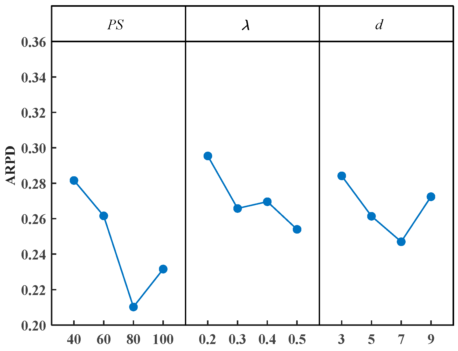
4.2. Parameter Configuration

The parameters of the DFFO algorithm include the population size PS, the elite population ratio $\lambda$, and the job length d. The parameter configurations are as follows: $PS\in \{40,60,80,100\}$, $\lambda \in \{0.2,0.3,0.4,0.5\}$, and $d\in \{3,5,7,9\}$. These three parameters result in a total of 4 × 4 × 4 = 64 different combination configurations. Using the same examples for algorithm calibration can lead to overfitting. To calibrate the parameters of the DFFO algorithm, the Taillard benchmark set [22] is used in this section. This dataset includes 12 groups of varying sizes, and each test instance is independently run 10 times. Additionally, a multivariate analysis of variance (ANOVA) method is employed to analyze the results.

Table 2. Results of multivariate analysis of variance parameters.

Source	Sum of Squares	Degrees of Freedom	Mean Square	F-Ratio	p-Value
$PS$	0.39	3	0.1894	1.32	0.0000
$\lambda$	181.26	3	35.2652	266.32	0.0000
$d$	5.32	3	0.8365	6.01	0.0000
$PS\ast \lambda$	2.03	9	0.2156	0.48	0.5489
$PS\ast d$	2.89	9	0.4856	0.52	0.6629
$\lambda \ast d$	4.16	9	0.2769	0.09	0.8413

presents the results of the multivariate analysis of variance, and Figure 4 shows the main effects plot for the parameters.

From Table 2, it can be observed that the p-values for the parameters PS, $\lambda$, and $d$ are all less than the 0.05 confidence level. This indicates that these three parameters significantly influence the algorithm’s performance. Based on the multivariate analysis of variance results in Table 2 and the F-ratio, it is evident that $\lambda$ has the greatest impact on the performance of the DFFO algorithm. This is because the proportion of the elite population contributes to enhancing the algorithm’s performance. The next most influential parameters are $d$ and PS. In combination with the main effects plot shown in Figure 4, the DFFO parameters are selected as follows: PS = 80, $\lambda$ = 0.3, and $d$ = 7.

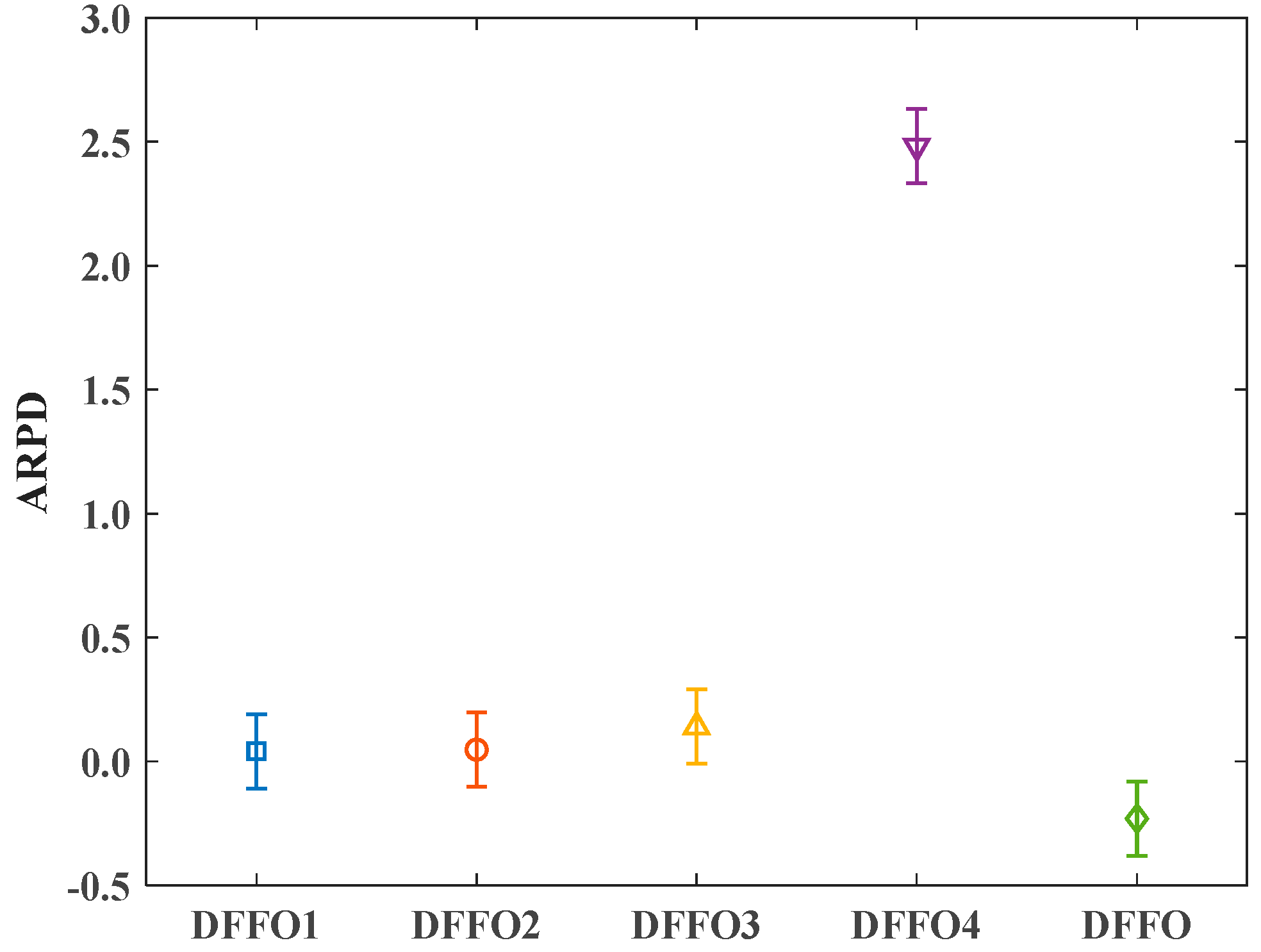
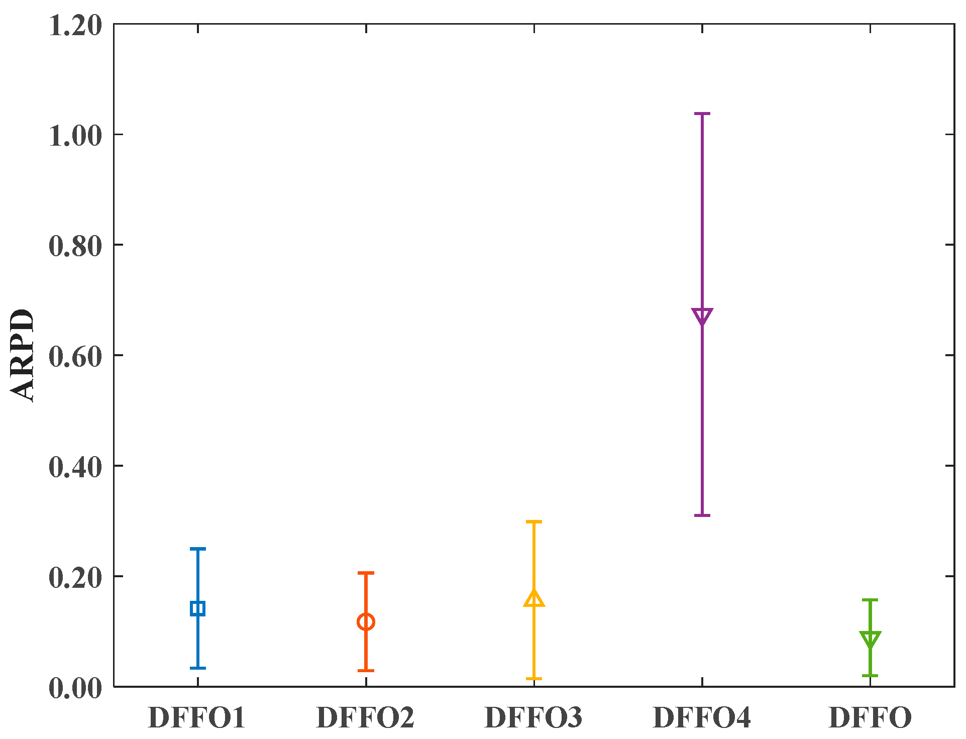
4.3. Performance Analysis of DFFO Components

This section validates the effectiveness of each component of the DFFO algorithm through experimental design. The DFFO algorithm mainly consists of the initialization strategy, the olfactory search phase based on variable neighborhoods, the visual search phase based on a probability model, and the local search strategy. To evaluate these components, the following variants are designed:

(1)

DFFO1: random initialization of the fruit fly population’s central positions.

(2)

DFFO2: replacing variable neighborhood search with single neighborhood search.

(3)

DFFO3: removing the visual search phase based on the probability model and using the original update mechanism of the algorithm.

(4)

DFFO4: removing the local search strategy.

The experimental setup remains the same as described earlier.

Table 3. APRD and SD values of DFFO and variant algorithms.

n	m	DFFO1		DFFO2		DFFO3		DFFO4		DFFO
		ARPD	SD	ARPD	SD	ARPD	SD	ARPD	SD	ARPD	SD
	10	0.184	0.091	0.214	0.221	0.417	0.218	3.446	0.965	0.123	0.095
50	20	0.080	0.130	0.008	0.107	0.452	0.273	4.241	1.235	0.036	0.128
	30	0.021	0.372	0.025	0.205	0.521	0.518	1.354	0.025	−0.070	0.190
	10	0.102	0.060	0.123	0.072	0.150	0.045	2.154	0.681	0.062	0.070
100	20	0.060	0.168	−0.018	0.231	0.156	0.184	3.050	1.201	−0.085	0.130
	30	−0.154	0.331	−0.133	0.296	0.276	0.405	4.903	1.201	−0.310	0.210
	10	0.004	0.002	0.008	0.003	0.008	0.002	0.717	0.356	0.003	0.002
150	20	0.093	0.150	0.185	0.093	0.232	0.167	3.265	0.686	0.001	0.088
	30	0.006	0.258	0.132	0.221	0.049	0.232	3.425	0.814	−0.178	0.165
	10	0.004	0.014	−0.001	0.010	0.022	0.055	0.472	0.252	−0.005	0.002
200	20	0.143	0.146	0.060	0.138	0.080	0.103	2.204	0.594	−0.001	0.108
	30	−0.096	0.235	−0.025	0.145	−0.011	0.239	3.394	0.701	−3.478	0.156
	10	0.004	0.014	−0.003	0.007	−0.005	0.004	0.478	0.256	−0.005	0.004
250	20	0.088	0.124	0.079	0.079	0.088	0.085	2.023	0.591	−0.010	0.005
	30	−0.020	0.165	−0.021	0.121	−0.059	0.126	3.381	1.083	−0.158	0.129
	10	0.001	0.001	0.003	0.004	0.006	0.012	0.628	0.254	0.000	0.002
300	20	0.098	0.095	0.112	0.056	0.046	0.012	2.364	0.487	−0.016	0.040
	30	0.132	0.195	0.116	0.108	0.099	0.140	3.175	0.745	−0.046	0.072
Mean		0.044	0.142	0.048	0.118	0.140	0.157	2.481	0.699	−0.230	0.088

presents the average relative percentage deviation (APRD) and standard deviation (SD) values obtained by the DFFO algorithm and its variants. To verify whether the conclusions are statistically significant, a multivariate analysis of variance (MANOVA) was conducted to test the differences in the experimental results in Table 3. Figure 5 shows the 95% confidence interval plot for each variant, and Figure 6 illustrates the variance interval plot for each variant.

From Table 3, it can be observed that the ARPD of the DFFO algorithm is −0.230, which is better than those of the other variants: DFFO1 (0.044), DFFO2 (0.048), DFFO3 (0.140), and DFFO4 (2.481). This demonstrates that each strategy contributes positively to the algorithm’s performance. Additionally, the DFFO algorithm has the smallest standard deviation, indicating that the combination of these strategies enhances the robustness of the algorithm. Furthermore, as shown in Figure 5, the intervals of DFFO and its variants do not overlap, and in Figure 6, the variance intervals of the variants show the smallest fluctuations. These observations validate the above conclusions.

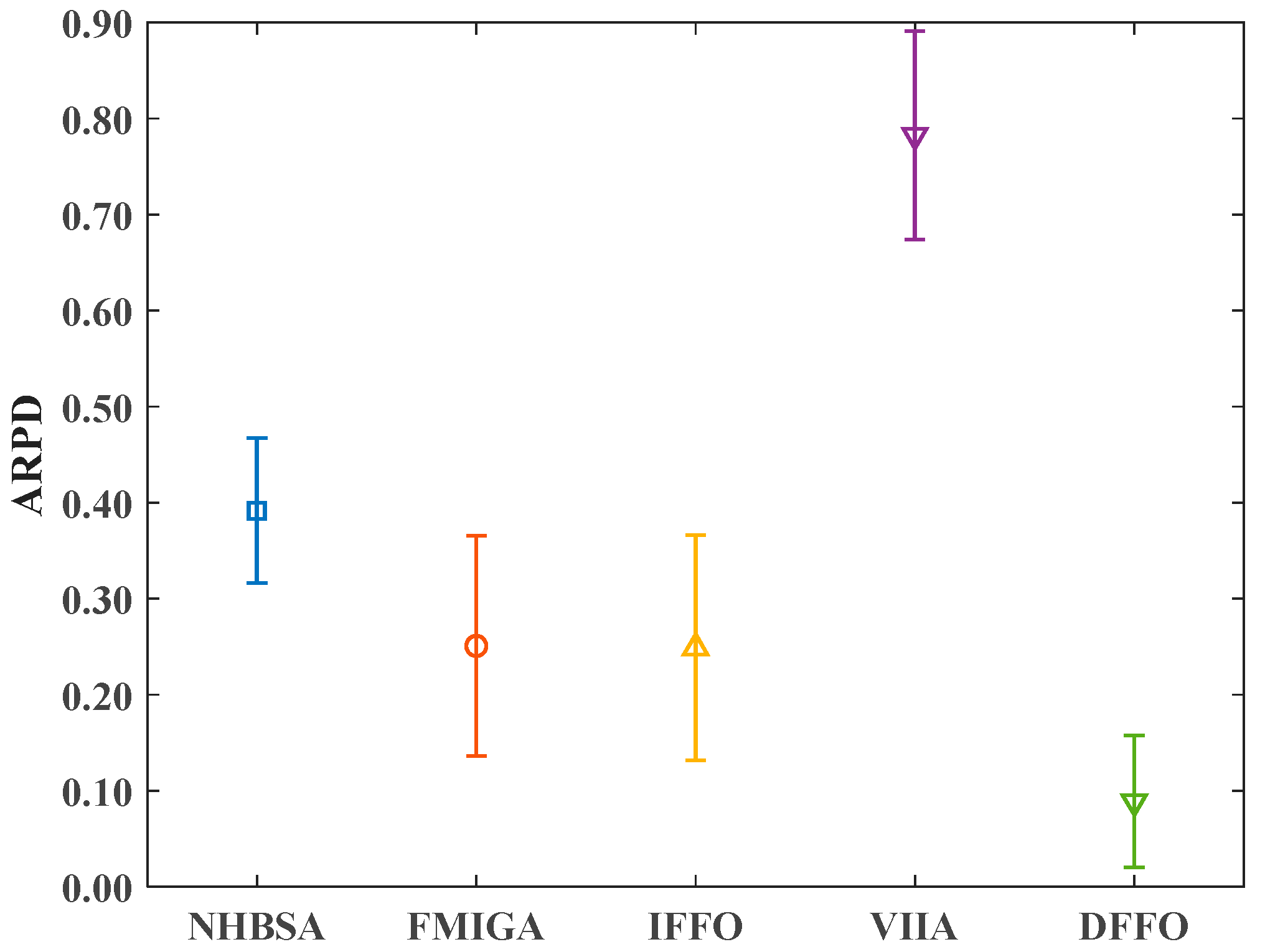
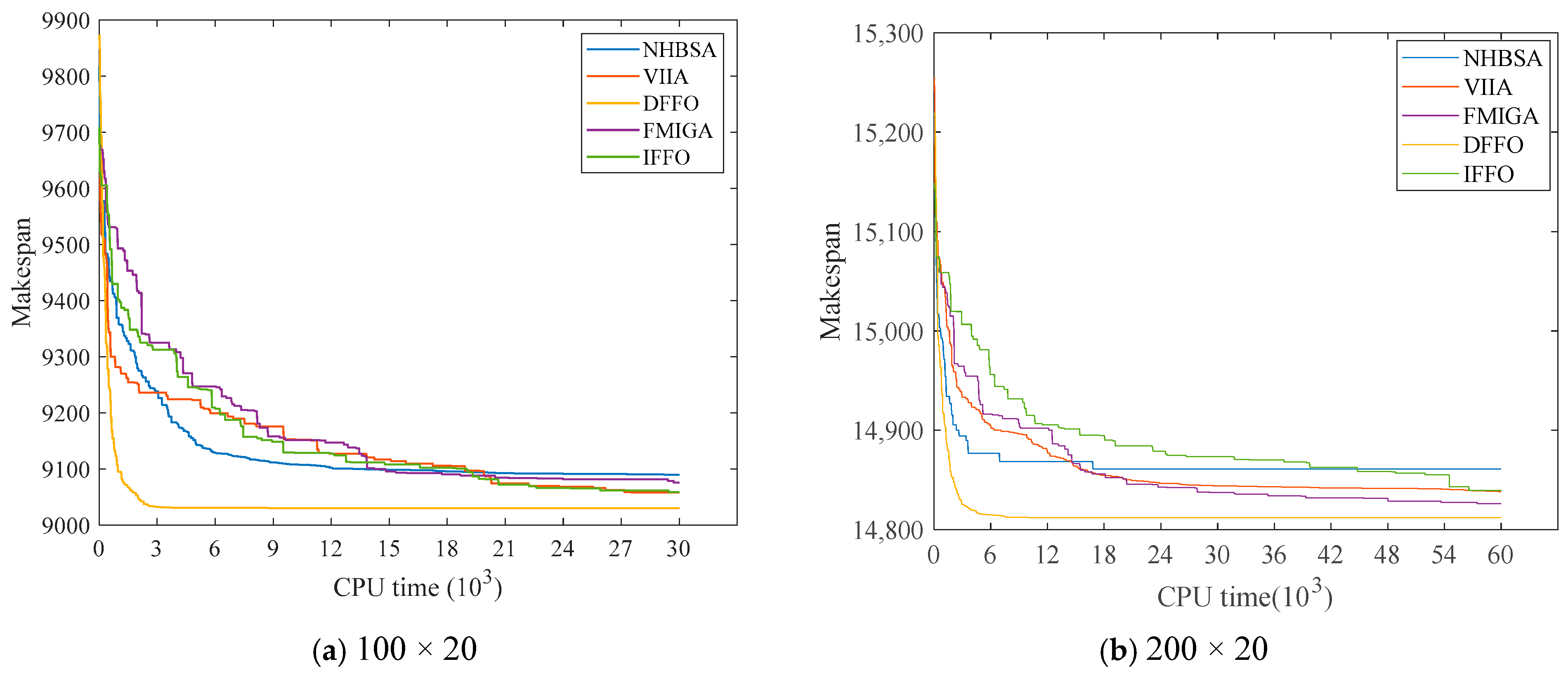
4.4. Comparative Analysis with Related Algorithms

In this section, DFFO is compared with more advanced algorithms for solving flow shop scheduling problems, such as novel hybrid bird swarm algorithm (NHBSA) [5], the forward-moving iterative greedy algorithm (FMIGA) [6], the improved fruit fly optimization algorithm (IFFO) [4], and the variable internal iterative algorithm (VIIA) [23]. In order to ensure the fairness of comparison, the parameter values of the comparison algorithm have been calibrated like those of the DFFO algorithm. For detailed values, see

Table 4. Parameter values of DFFO and comparison algorithm.

Algorithm	Parameter Value
NHBSA	PS = 80, learning factor c1 = 0.5, and learning factor c2 = 0.5
FGMIGA	PS = 80 and $d$ = 7
IFFO	PS = 80 and local search times LS = 10
VIIA	PS = 80 and $d$ = 7
DFFO	PS = 80, $\lambda$ = 0.3, and $d$ = 7

. The experimental setup remains the same as described previously.

Table 5. DFFO and APRD values of the comparison algorithm.

n	m	NHBSA		FMIGA		IFFO		VIIA		DFFO
		ARPD	SD	ARPD	SD	ARPD	SD	ARPD	SD	ARPD	SD
	10	0.479	0.415	0.442	0.299	0.353	0.289	0.542	0.709	0.123	0.095
50	20	1.586	0.284	0.387	0.186	0.321	0.183	1.158	0.673	0.036	0.128
	30	0.583	0.344	0.574	0.180	0.792	0.188	0.216	0.801	−0.070	0.190
	10	0.154	0.435	0.243	0.195	0.187	0.169	0.090	0.855	0.062	0.070
100	20	0.319	0.302	0.299	0.192	0.177	0.157	0.158	0.563	−0.085	0.130
	30	0.508	0.343	0.631	0.202	0.210	0.210	0.243	0.805	−0.310	0.210
	10	0.005	0.346	0.034	0.229	0.009	0.559	0.020	0.753	0.003	0.002
150	20	0.394	0.479	0.385	0.247	−0.044	0.283	−0.127	0.919	0.001	0.088
	30	0.257	0.349	0.287	0.577	0.184	0.195	0.194	0.819	−0.178	0.165
	10	0.006	0.463	0.058	0.283	0.010	0.337	0.000	0.907	−0.005	0.002
200	20	0.103	0.455	0.274	0.178	0.192	0.221	0.124	0.931	−0.001	0.108
	30	0.119	0.319	0.250	0.194	0.091	0.164	0.001	0.699	−3.478	0.156
	10	0.006	0.406	0.051	0.195	0.040	0.188	0.035	0.941	−0.005	0.004
250	20	0.135	0.316	0.181	0.190	0.089	0.233	0.067	0.597	−0.010	0.005
	30	0.124	0.434	0.350	0.330	0.070	0.300	−0.012	0.816	−0.158	0.129
	10	0.001	0.486	0.044	0.226	0.414	0.199	0.103	0.803	0.000	0.002
300	20	0.162	0.326	0.223	0.154	0.129	0.162	0.087	0.754	−0.016	0.040
	30	0.239	0.348	0.420	0.156	0.155	0.147	0.181	0.741	−0.046	0.072
Mean		0.288	0.142	0.285	0.118	0.188	0.157	0.171	0.699	−0.230	0.088

presents the ARPD values of DFFO and the other comparative algorithms.

To verify the statistical significance of these conclusions, ANOVA was conducted on the experimental results in Table 5. Figure 6 shows the 95% confidence interval plot for each algorithm variant.

From Table 5, it can be observed that the ARPD of the DFFO algorithm is −0.230, which outperforms NHBSA (0.288), FMIGA (0.285), IFFO (0.188), and VIIA (0.171). This indicates that the DFFO algorithm is superior to the compared algorithms.

As shown in Figure 7, the intervals of DFFO and the comparative algorithms do not overlap, demonstrating that the DFFO algorithm exhibits statistically significant differences from the other algorithms. Additionally, from Figure 8, the variance intervals of DFFO and the comparative algorithms show the smallest fluctuations, further indicating that the DFFO algorithm has better robustness compared with the other algorithms.

Additionally, Figure 9 presents the convergence curves of DFFO, NHBSA, FMIGA, VIIA, and IFFO algorithms on large-scale test instances. From Figure 9, it can be observed that the overall performance of the DFFO algorithm is significantly better than that of NHBSA, FMIGA, VIIA, and IFFO on the two large-scale test instances. Moreover, as the problem scale increases, the advantages of DFFO become increasingly pronounced. Based on the experimental results mentioned above, the DFFO algorithm demonstrates greater competitiveness compared with other peer algorithms.

4.5. Experimental Summary

This section focuses on a summary of the above experiments. In order to demonstrate the effectiveness of the DFFO algorithm, the parameters of the DFFO algorithm are first calibrated (Section 4.2), then the performance of the components of the DFFO algorithm is analyzed (Section 4.3), and finally the accuracy and stability of the most advanced algorithms are tested (Section 4.4). After the above operation, it is proved that the DFFO algorithm is superior to the NHBSA, FMIGA, VIIA, and IFFO algorithms in convergence speed, precision, and robustness. Especially when solving the actual production scheduling problem, all the algorithms are under the same stopping criterion. The experimental results show that the performance of the DFFO algorithm is at least 28.1% better than the other algorithms, thus verifying the effectiveness of the DFFO algorithm.

Based on the above experimental results, the effectiveness of the DFFO algorithm is verified. On the one hand, DFFO guides bees to approach the real optimal solution by using specific problem operators and effective strategies. On the other hand, the evolutionary mechanism of DFFO can ensure the distribution of solutions as much as possible. Finally, the experimental results show that the MABC algorithm is more competitive than the other algorithms.

5. Conclusions

This paper proposes a DFFO algorithm to solve the NIPFSP. DFFO consists of three phases, i.e., the smell search phase based on the variable neighborhood, the visual search phase based on the probabilistic model, and the local search phase. In the smell search phase, multiple perturbation operators are constructed to further expand the search range of the solution; in the visual search phase, a probabilistic model is constructed to generate a series of positional sequences using some elite groups, and the concept of shared sequences is adopted to generate new individuals based on the positional sequences and shared sequences. In the local search stage, the optimal individuals are refined with the help of an iterative greedy algorithm, so that the fruit flies are directed to more promising regions. Finally, the test results show that DFFO’s performance is at least 28.1% better than other algorithms, which verifies that DFFO is an efficient method to solve the NIPFSP.

Since the DFFO algorithm’s evolutionary operators were designed based on the specific characteristics of the problem, it has certain limitations and may not be directly applicable to other scheduling problems. However, it provides valuable insights for solving other scheduling challenges.

For future research, we aim to integrate different strategies, such as combining deep reinforcement learning, into the fruit fly optimization framework to address multi-objective scheduling problems, path planning problems, and integrated scheduling issues. This is one of the directions we are actively pursuing.

References

1. Fernandez-Viagas, V.; Molina-Pariente, J.M.; Framinan, J.M. Generalised accelerations for insertion-based heuristics in permutation flowshop scheduling. Eur. J. Oper. Res. 2020, 282, 858–872. [Google Scholar] [CrossRef]
2. Bagheri Rad, N.; Behnamian, J. Recent trends in distributed production network scheduling problem. Artif. Intell. Rev. 2022, 55, 2945–2995. [Google Scholar] [CrossRef]
3. Huang, J.P.; Pan, Q.K.; Gao, L. An effective iterated greedy method for the distributed permutation flowshop scheduling problem with sequence-dependent setup times. Swarm Evol. Comput. 2020, 59, 100742. [Google Scholar] [CrossRef]
4. Yin, R.X.; Feng, X.Q.; Wu, T. Improved fruit fly algorithm for no idle flow shop scheduling problem. Modul. Mach. Tool Autom. Manuf. Technol. 2022, 32, 142–150. [Google Scholar]
5. Yan, H.C.; Tang, W.; Yao, B. New hybrid bird swarm Algorithm for no idle flow shop scheduling Problem. Microelectron. Comput. 2022, 39, 98–106. [Google Scholar]
6. Zhao, Z.M.; Wang, J.H.; Zhu, K. Minimum iterative greedy algorithm for total delay in no-idle permutation flow shop. Modul. Mach. Tool Autom. Process. Technol. 2023, 3, 177–182. [Google Scholar]
7. Zhao, R.; Lang, J.; Gu, X.S. Hybrid no-idle permutation flow shop scheduling based on multi-objective discrete sine optimization algorithm. J. East China Univ. Sci. Technol. (Nat. Sci. Ed.) 2022, 48, 76–86. [Google Scholar]
8. Pei, X.B.; Li, Y.Z. Application of improved hybrid evolutionary Algorithm to no-idle permutation flow shop scheduling problem. Oper. Res. Manag. 2019, 29, 204–212. [Google Scholar]
9. Pan, W.T. A new fruit fly optimization algorithm: Taking the financial distress model as an example. Knowl.-Based Syst. 2012, 26, 69–74. [Google Scholar] [CrossRef]
10. Wang, L.; Xiong, Y.N.; Li, S.; Zeng, Y.R. New fruit fly optimization algorithm with joint search strategies for function optimization problems. Knowl.-Based Syst. 2021, 176, 77–96. [Google Scholar] [CrossRef]
11. Ibrahim, I.A.; Hossain, M.J.; Duck, B.C. A hybrid wind driven-based fruit fly optimization algorithm for identifying the parameters of a double-diode photovoltaic cell model considering degradation effects. Sustain. Energy Technol. Assess. 2022, 50, 101685. [Google Scholar] [CrossRef]
12. Saminathan, K.; Thangavel, R. Energy efficient and delay aware clustering in mobile adhoc network: A hybrid fruit fly optimization algorithm and whale optimization algorithm approach. Concurr. Comput. Pract. Exp. 2022, 34, 6867. [Google Scholar] [CrossRef]
13. Hu, G.; Xu, Z.; Wang, G.; Zeng, B.; Liu, Y.; Lei, Y. Forecasting energy consumption of long-distance oil products pipeline based on improved fruit fly optimization algorithm and support vector regression. Energy 2021, 224, 120153. [Google Scholar] [CrossRef]
14. Zhu, N.; Zhao, F.; Wang, L.; Ding, R.; Xu, T. A discrete learning fruit fly algorithm based on knowledge for the distributed no-wait flow shop scheduling with due windows. Expert Syst. Appl. 2022, 198, 116921. [Google Scholar] [CrossRef]
15. Guo, H.W.; Sang, H.Y.; Zhang, B.; Meng, L.L.; Liu, L.L. An effective metaheuristic with a differential flight strategy for the distributed permutation flowshop scheduling problem with sequence-dependent setup times. Knowl.-Based Syst. 2022, 242, 108328. [Google Scholar] [CrossRef]
16. Guo, H.W.; Sang, H.Y.; Zhang, X.J.; Duan, P.; Li, J.Q.; Han, Y.Y. An effective fruit fly optimization algorithm for the distributed permutation flowshop scheduling problem with total flowtime. Eng. Appl. Artif. Intell. 2023, 123, 106347. [Google Scholar] [CrossRef]
17. Namaz, M.; Enscore, E.; Ham, I. A heuristic algorithm for the m-machine, n-job flow-shop sequencing problem. Omega 1983, 11, 91–95. [Google Scholar]
18. Ceberio, J.; Irurozki, E.; Mendiburu, A.; Lozano, J.A. A distance-based ranking model estimation of distribution algorithm for the flowshop scheduling problem. IEEE Trans. Evol. Comput. 2014, 18, 286–300. [Google Scholar] [CrossRef]
19. Wang, S.Y.; Wang, L.; Liu, M.; Xu, Y. An order-based estimation of distribution algorithm for stochastic hybrid flow-shop scheduling problem. Int. J. Comput. Integr. Manuf. 2014, 28, 307–320. [Google Scholar] [CrossRef]
20. Ruiz, R.; Thoama, S. A simple and effective iterated greedy algorithm for the permutation flowshop scheduling problem. Eur. J. Oper. Res. 2007, 177, 2033–2049. [Google Scholar] [CrossRef]
21. Ruiz, R.; Vallada, E.; Fernandez-Martinez, C. Scheduling in flowshops with no-idle machines. In Computational Intelligence in Flow Shop and Job Shop Scheduling; Springer: Berlin/Heidelberg, Germany, 2009; pp. 21–51. [Google Scholar]
22. Taillard, E. Benchmarks for basic scheduling problems. Eur. J. Oper. Res. 1993, 64, 278–285. [Google Scholar] [CrossRef]
23. Li, J.; Li, Y.W. Variable block internal iteration algorithm for no idle flow shop problem. Appl. Res. Comput. 2022, 39, 3667–3672. [Google Scholar]
Figure 1. DFFO flow chart.
Processes 13 00476 g001
Figure 2. Four kinds of neighborhood perturbation operators.
Processes 13 00476 g002
Figure 3. Local search process.
Processes 13 00476 g003
Figure 4. Main effect diagram of DFFO parameters.
Processes 13 00476 g004
Figure 5. The 95% confidence intervals for DFFO and variants.
Processes 13 00476 g005
Figure 6. Variogram of DFFO and each variation.
Processes 13 00476 g006
Figure 7. The 95% confidence interval diagram of DFFO and comparison algorithm.
Processes 13 00476 g007
Figure 8. Variance interval diagram of DFFO and comparison algorithm.
Processes 13 00476 g008
Figure 9. Convergence diagram on a DFFO large-scale test instance.
Processes 13 00476 g009