Abstract
When a single-phase grounding fault occurs in a resonant grounding system, due to the compensation effect of the arc coil on the system, there are problems such as the fault signal amplitude and the signal waveform being close, which leads to difficulties in line selection. This paper proposes a fault line selection discrimination method based on MCEEMD-MPE normalization and a k-means clustering analysis algorithm. The method is applied to the single-phase grounding fault of a resonant grounding system. The zero-sequence current is obtained and decomposed by MCCEEMD to obtain a number of components. The components with obvious characteristics are selected for normalization calculation by multi-scale permutation entropy, which not only avoids mode aliasing, but also highlights the characteristics of the fault signal at different scales. Finally, the k-means clustering analysis algorithm is used to correctly distinguish the fault and non-fault lines. The effectiveness of the method is verified in a real test field case. The results of the calculation show that the method can accurately identify the fault line under different faults when a single-phase grounding fault occurs. The recognition accuracy is 100%, which effectively improves the grounding fault line selection rate of the resonant grounding.
1. Introduction
Among the common faults in distribution networks, single-phase grounding faults are the most frequent [1]. When a single-phase grounding fault occurs in a 6–35 kV resonant grounding (neutral point grounded an arc suppression coil) system [2], the distribution system is affected, resulting in line damage. The capacitive current to ground each phase increases accordingly, this also increases the capacitive current to ground at the fault point, resulting in the system line being prone to arc overvoltage [3]. In order to effectively prevent resonance overvoltage and arc hazards, the overcompensation method is used to solve these problems [4]. Due to the brief transient process that occurs after a single-phase grounding fault in a resonant grounding system, the fault current changes very little, especially when a high-resistance grounding fault occurs. The fault characteristics become very weak and the state is mixed, which not only increases the difficulty in line selection, but also causes difficulties in selecting appropriate technologies [5]. Therefore, when a grounding fault occurs, the steady-state and transient processes of the fault signal are analyzed separately. First, due to the influence of the arc suppression coil, the fault steady-state current is weak, unstable, and easily disturbed. The traditional state electrical quantity fault detection method cannot accurately identify the fault line, which can easily lead to the fault quantity feature change not being prominent enough. Because the change is not obvious, significant detection result errors, etc., can occur [6]. However, there is a significant amount of transient information in the transient process, which is more conducive for line selection [7]. It is common to use signal processing to deal with fault signals in research. In [8,9], diagnosis and processing were used when faults occurred in subsea production systems. The former proposed a fault diagnosis framework that was both digital and model-driven, which was used obtain status times when the subsea production system failed, in order to ensure the smooth production of oil and gas. The latter combined extracted data to establish a fault diagnosis model and effectively judge faults in system operation through the processing of fault data. Therefore, effective signal processing methods can be used to extract fault characteristics and quickly find the fault line, which greatly saves the time of line selection and the success rate of fault line selection [10].
In fault line selection, methods such as empirical mode decomposition (EMD), Fourier transform (FT), wavelet transform (WT), and Hilbertuang transform (HHT) are used to extract fault factors from time-domain and frequency-domain information [11]; however, there are disadvantages to these methods such as unstable decomposition and unclear changes when processing nonlinear and nonstationary signals [12].
Reference [13] introduced the use of empirical mode decomposition (EMD) to decompose the transient characteristics of the line; however, when the line appears to be noise-intensive, mode aliasing can occur, which is not suitable for resolving the line content. Integrated empirical mode decomposition (EEMD) is an improved version of EMD [14]; however, its ability to reduce mode aliasing is limited, and the signal after decomposition may also have some residual errors. Complementary ensemble empirical mode decomposition (CEEMD) is based on the integration of empirical mode decomposition (EEMD) to increase the inverse white noise and the integration of average processing [15]; although this can alleviate the reconstruction error, error accumulation caused by too many decomposition components results in the low accuracy of the IMF as a whole. The improved complementary ensemble empirical mode decomposition (MCEEMD), based on CEEMD, is used to reconstruct frequency and amplitude similar components [16]. It can accurately show the decomposition integrity of the fault line because it can successfully inhibit mode aliasing and reduce the pseudo-component, eliminate the unnecessary integration average in CEEMD, and reduce the computational scale of CEEMD, thereby avoiding the component reconstruction error in the decomposition process. References [17,18] demonstrated the outstanding efficacy of the MCEEMD technique. According to the extracted oscillatory instance signals, signals were decomposed by EMD, EEMD, CEEMD and MCEEMD, respectively. The results of the research showed that MCEEMD exhibited improved power levels, reduced noise disturbances, and had significant advantages in suppressing mode splitting and noise residuals. Reference [19] used the MCEEMD algorithm to decompose and compare a fault signal at different degrees, which effectively verified the effectiveness of the algorithm at suppressing modal decomposition mixing.
Entropy, which can reflect the complexity of a signal, is generally used as an index to construct nonlinear and non-stationary data feature vectors [20] such as PE or MPE. The PE algorithm has the capability to identify complexity and mutations within time series and to quantize time complexity into entropy to realize phase space reconstruction; it is characterized by a fast calculation time and strong anti-interference ability [21]; however, the permutation entropy algorithm has some limitations and is only suitable for detecting single-scale randomness [22]. MPE is a kind of sample entropy that analyzes different scales in time series [23]. MPE possesses the benefits of straightforward calculation, formidable interference resistance and flexibility, and can measure the randomness of different scales [24]. Fault signals contain different important information at different scales; therefore, it is more suitable to analyze the fault signal by choosing the best parameters of the MPE to calculate the analysis signal skew mean as the fault characteristic parameter.
After extracting the feature vector effectively in different fault cases, a fault pattern can be recognized using a high-performance multi-classifier. Cluster analysis is a classical mathematical statistics method in common use [25]. Cluster analysis is mainly used in the classification range according to the characteristics of the object classification [26]. The k-means clustering analysis algorithm is both straightforward and rapid [27] and adheres to a distinct partition concept, converting data clustering into a nonlinear optimization challenge. According to the principle of minimum distance from the initial center point, all the data are divided into classes where the centers are located. Solutions are obtained mainly by solving the problem of the distance between the initial fault clusters [28].
Based on the above description, this paper proposes a method of line selection that combines MCEEMD-MPE normalization with a k-means clustering algorithm. The method first suppresses the modal splitting and noise residue generated by the grounding fault signal by combining the median and mean operators in the ensemble process using the MCEEMD algorithm, avoiding the mode aliasing caused by data reconstruction. Second, the MPE algorithm is used to extract the fault signal information and reconstruct the signal entropy value, which is normalized to better reflect the characteristics of the fault signal. Finally, the k-means clustering analysis algorithm is used to correctly distinguish the fault and non-fault lines. The effectiveness of the method was verified in a real test field case. The paper is organized as follows: Section 2 introduces the decomposition principle of the algorithm and the fault line selection flow chart; Section 3 outlines the principle of the transient analysis of single-phase grounding in a resonant grounding system and the simulation experiment of the established model; Section 4 introduces the verification of the proposed method in a real test field case as well as a comparative analysis with other algorithms; and Section 5 is the conclusion.
2. Algorithm Principle
2.1. MCEEMD Decomposition Principle
The MCEEMD decomposition steps are shown below.
(1) Set the initial data to 0 white noise and add it to the original signal to obtain the following expression:
The amplitude of the noise is , for setting the logarithm of the white noise, . The calculated and are decomposed by EMD, and the first-order IMF components and are obtained, which are .
(2) The IMF component is obtained by the integrated mean decomposition step (1).
(3) If the entropy value of the actual signal does not exceed , it is considered to be stable; If the signal entropy value exceeds , it is regarded as an anomaly. The calculation of the repeated step (1) tends to make the IMF component stable and is regarded as a non-anomaly, as follows:
(4) The original signal is subtracted from the pre-p-1 IMF component of the integrated mean decomposition to obtain the residual component .
(5) The residual signal is repeated in steps (1) and (2), and the obtained parts of the decomposition are arranged according to the frequency from high to low.
2.2. MPE Standardized Decomposition Principle
MPE is an improvement of PE, which is used to coarsen the time series at multiple scales and then calculate the PE value of each coarseained time series. Compared with the ability to distinguish the irregularity and complexity of different granularities of linear signals, it can better distinguish the feature values of fault characteristics of fault lines [29].
2.2.1. Specific Decomposition Steps for MPE
(1) Set a group of time series for multi-scale coarse-graining to obtain the following formula:
In Formula (5), S is the time scale factor and is the multi-scale time series. When , the coarse-graining sequence is the original time series. When , the coarse-graining sequence is is .
(2) The time series reconstruction of is as follows:
In the above Formula (6), represents the delay time, while m denotes the embedding dimension.
(3) The ascending permutation of the reconstructed sequence is carried out, and the m! species permutation is obtained. Set the number of times the different arrangements appear for , the probability is , as follows, in Formulas (7) and (8):
(4) The permutation entropy is calculated and normalized as follows:
In Formula (9), is the calculated permutation entropy. The closer the entropy value H is to 1, the higher the randomness of the signal and the higher the non-stationarity.
2.2.2. Parameter Selection for the MPE
MPE has three parameters to be selected: the embedding dimension m; time scale s; and time delay . According to the analysis conducted by reference [30], the influence of time delay on time series calculation is small, and is usually set as 1. There is no uniform standard for time scale s; therefore, this paper chooses s = 4 [31]. According to reference [32], too many embedded bits m will lead to too many uniform permutation states, and too few embedded bits m will lead to confusion of the permutation states, which cannot then be distinguished. Therefore, choosing M = 6 can better reflect the scale factor advantage.
2.2.3. MPE Normalization
The calculated multi-scale permutation entropy is normalized by using the Z-score [33], which is transformed using the mean and variance methods to conform to the normal distribution of the elements [34], with the following formula:
In the formula above, is the multi-scale arrangement of entropy data, is the normalized pre-processed entropy data, x is the entropy mean, and S is the entropy standard deviation.
2.3. K-Means Clustering Analysis Principle
The k-means algorithm takes the following steps:
(1) Constructing the initial signal matrix x = [x1, x2, …, xn], set the number of categories of k. The k value is mainly set according to the actual specific sample in [35], while the main goal in this paper is to distinguish fault signals from non-fault signals; therefore, this paper set the cluster value as k = 2;
(2) The sum of the distances from each signal point to the cluster center is the objective function, as follows:
where ; , is the central part of the cluster in the initial category, and is the sample set of the first category after clustering;
(3) The calculation in Formula (13) is updated continuously until it converges and a new cluster center point is obtained.
2.4. Model Solving Algorithm and Process
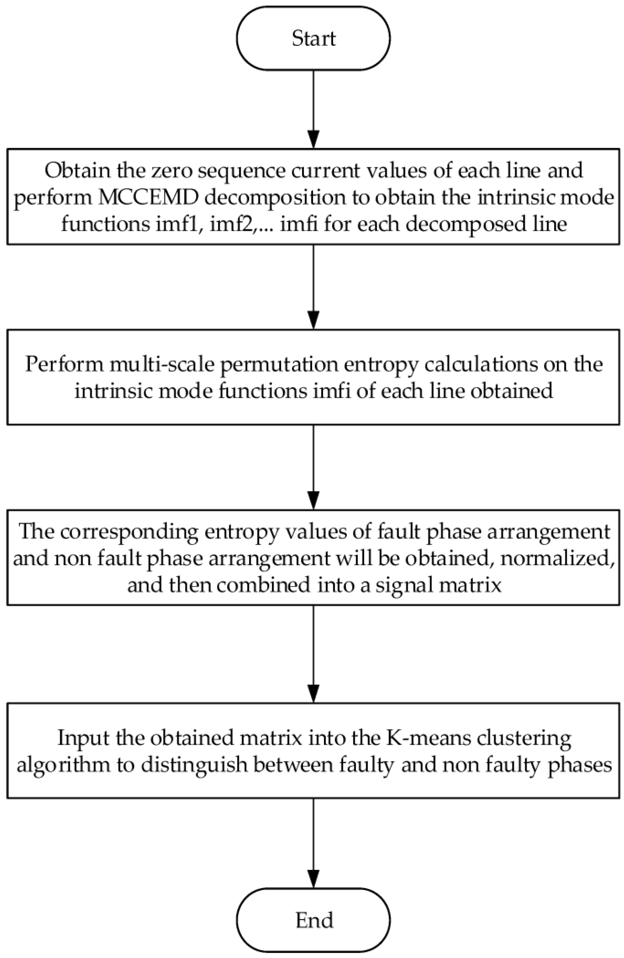
Figure 1 illustrates the process involved in selecting single-phase-to-ground fault lines for resonant grounding systems. The primary procedures are follows:
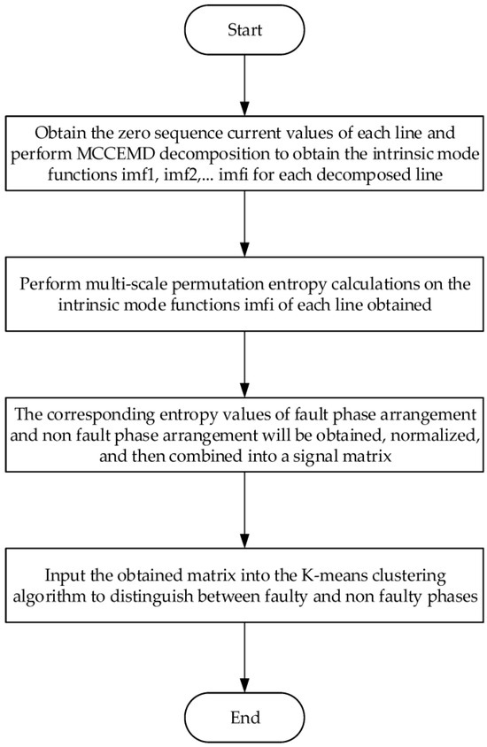
Figure 1.
Single-phase-to-ground fault line selection flow chart based on MCEEMD-MPE normalization and k-means clustering algorithm.
Step 1: The model components IMF1, IMF2, IMF3, among others, are obtained by decomposing each line of zero-sequence current signal;
Step 2: The zero-sequence current signal from each line is decomposed using MCCEMD to obtain mode components IMF1, IMF2, IMF3, and so on;
Step 3: The modal functions of each line are determined using IMF and the entropy values for both fault and non-fault phases are calculated. These multi-scale permutation entropy values are then normalized to form a signal matrix;
Step 4: The fault and non-fault lines are separated using the k-means clustering algorithm.
3. Transient Analysis of Single-Phase Grounding of Resonant Grounding System
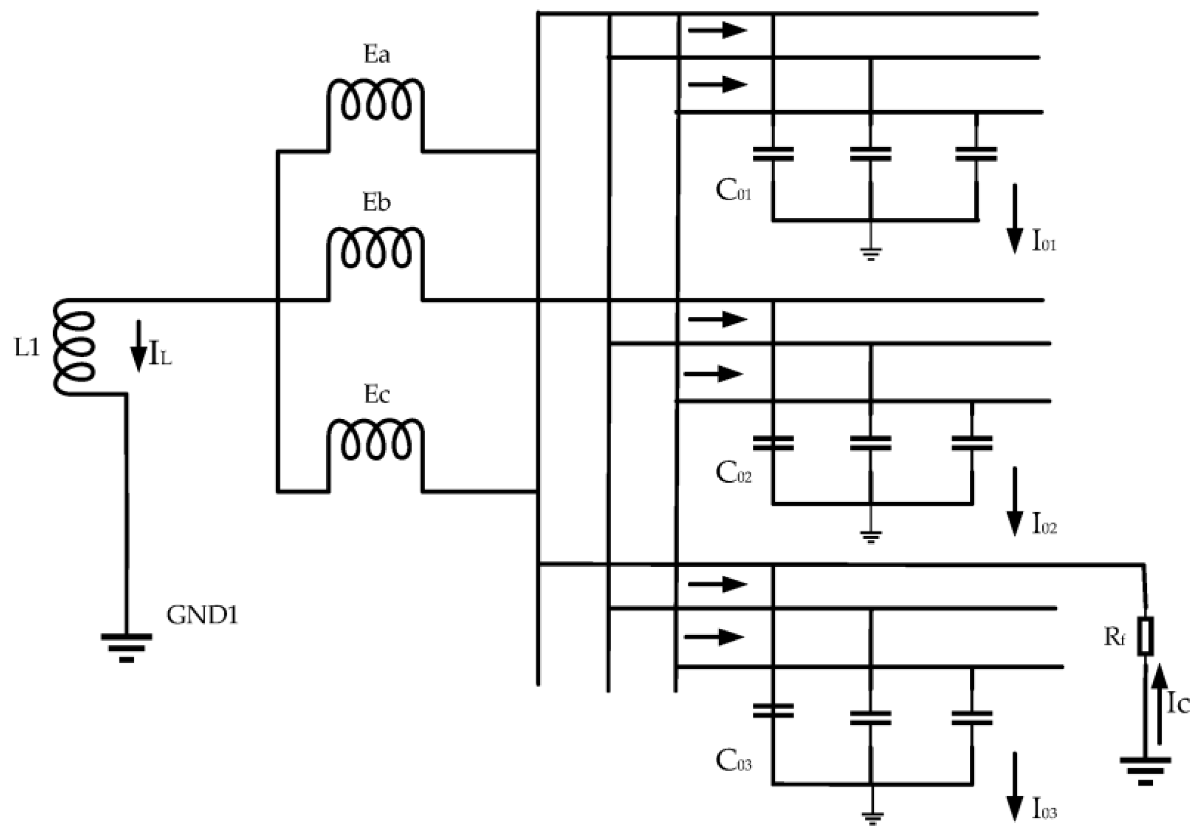
Figure 2 shows the single-phase-to-ground fault diagram of the resonant grounding system. is the equivalent voltage source, L1 is the arc suppression coil, and is the capacitance of the feed line to ground.

Figure 2.
Diagram illustrating the single-phase grounding fault in the resonant grounding system.
3.1. Steady-State Fault Characteristics
From Figure 2, it can be seen that the grounding current in the steady-state system mainly consists of two parts: the capacitive current in the circuit and the inductive current in the arc suppression coil. The fault grounding current is the sum of the line capacitance current and the inductance current; its relationship expression (14) is as follows:
In Formula (14), is expressed as the inductive current, is expressed as the capacitive current, and is expressed as the fault grounding current.
At this point, the voltage values in the line and the arc suppression coil have the same voltage value, but in the opposite direction. At this point the relationship is expressed as follows (15):
Define the compensation degree k as the proportion between the capacitance current and the inductance current and the expression is as follows (16):
When k > 1, the system is over-compensated. When k = 1, the line capacitance current and the inductance current in the arc suppression coil cancel each other out and the system exists in a state of resonance. When k < 1, the system is under-compensated.
3.2. Transient Period Fault Analysis
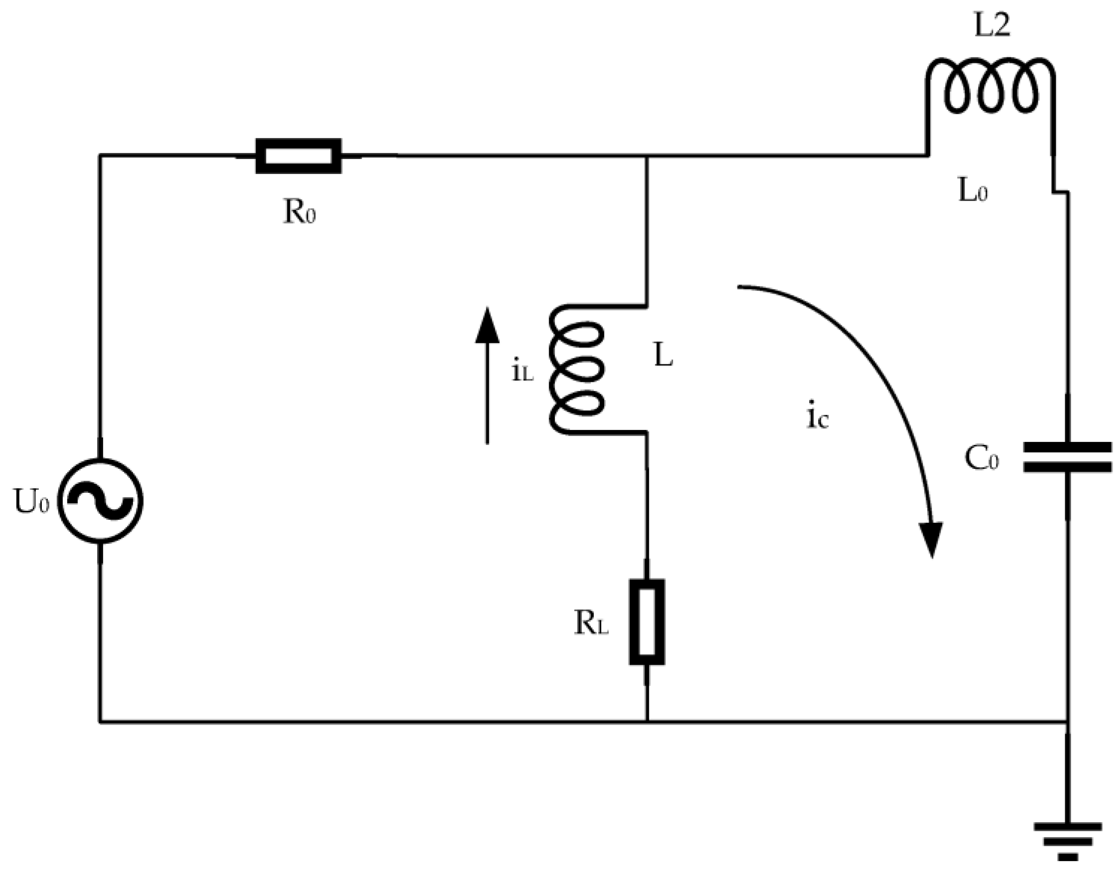
In a stable state, the magnitude of the zero-sequence current is minimal, and the characteristic change remains unclear, which adversely affects the selection of fault lines. The variations in current amplitude in the transient period are more obvious than those in the steady period, the fluctuations in current amplitude are more favorable for accurate fault line selection. Upon the system's grounding, the single-phase-to-ground fault equivalent circuit diagram is used to represent the transient process of the fault, as shown in Figure 3. In the diagram, R0 is the equivalent resistance of the zero-sequence current flowing through the circuit; L0 is the equivalent inductance of the circuit; C0 is the capacitance to ground of each circuit; RL is the resistance of the arc suppression coil; L is the inductance of the arc suppression coil; U0 is the equivalent zero-sequence voltage; ic is the capacitive current; and iL is the inductive current.

Figure 3.
Equivalent circuit of single-phase grounding fault in resonant grounding system.
(1) Transient to ground capacitance current. The formula is calculated and deduced according to Kirchhoff's voltage law and is shown in Formula (17), as follows:
In Formula (17), is the system angular frequency and is the fault closing angle [36].
When , the transient zero-sequence current behaves as a periodic oscillation with attenuation, and the free component in the circuit tends to be stable. When , the transient zero-sequence current behaves as a periodic oscillation with attenuation to stabilize the power frequency component. When the value of the failure closing angle is or , it is the highest value.
(2) Transient inductance current. At the moment of the fault, the inductive current in the inductance coil of the line has not appeared. It is set to the initial state at this time. The inductance current in the differential equation is calculated as follows (18):
In Formula (18), is the amplitude of the inductance current and is the time constant.
(3) Transient grounding current. The inductance current and capacitance are calculated in Formulas (17) and (18); thus, the formula for calculating the transient grounding current is derived as follows (19):
From the above formula, it can be concluded that fault angle affects the magnitude of the transient grounding current. When , the inductance current , the capacitance current . When , the capacitance current and the inductance current .
3.3. Fault Feature Analysis and Entropy Evaluation
This paper utilized the Simulink simulation program to construct a 10 kV resonant grounding system model in MATLAB (MathWorks company, Natick, MA, USA, Version number: matlab 2020a). The positive and negative sequence parameters of the three outgoing lines are R = 0.27 Ω, L = 2.55 × 10⁻⁴ H, C = 3.39 × 10⁻⁷ F, and the zero-sequence parameters are R0 = 2.7 Ω, L0 = 1.109 × 10⁻⁴ H, C0 = 2.8 × 10⁻⁷ F, respectively. The arc suppression coil adopts an over-compensation mode; the degree of compensation stands at 10%. The length of Line 1 is 7 km, Line 2 is 8 km and Line 3 is 9 km. At the same time, set Line 3 occurred A grounding fault, fault time set to 0.1 s for its simulation.
(1) The fault signal is decomposed by MCCEMD
There are many reasons for a short circuit, including component damage, such as equipment insulation aging, weather conditions, and man-made damage, etc. Therefore, the normalized multi-scale permutation entropy values of the zero-sequence current are calculated by setting the fault values of different grounding resistances as metallic grounding, 100 ω, 500 ω, 1000 ω, and 2000 ω, and the fault distances as 6 km, respectively. In a single-phase-to-ground fault system, the initial phase angle also has a significant impact on the transient inductance current. Therefore, the initial phase angle is set at , , and to calculate the normalized multi-scale permutation entropy of the zero-sequence current.
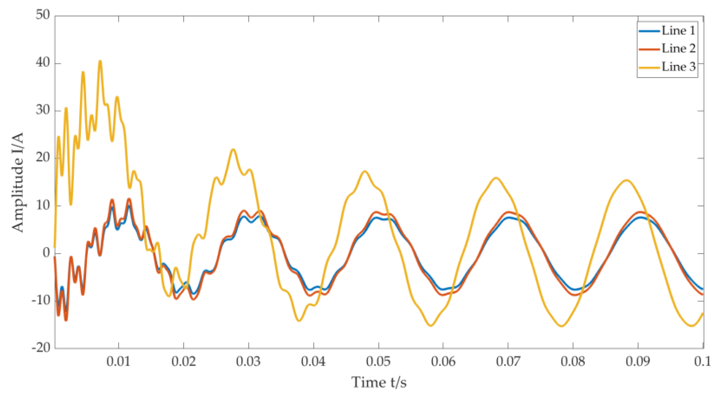
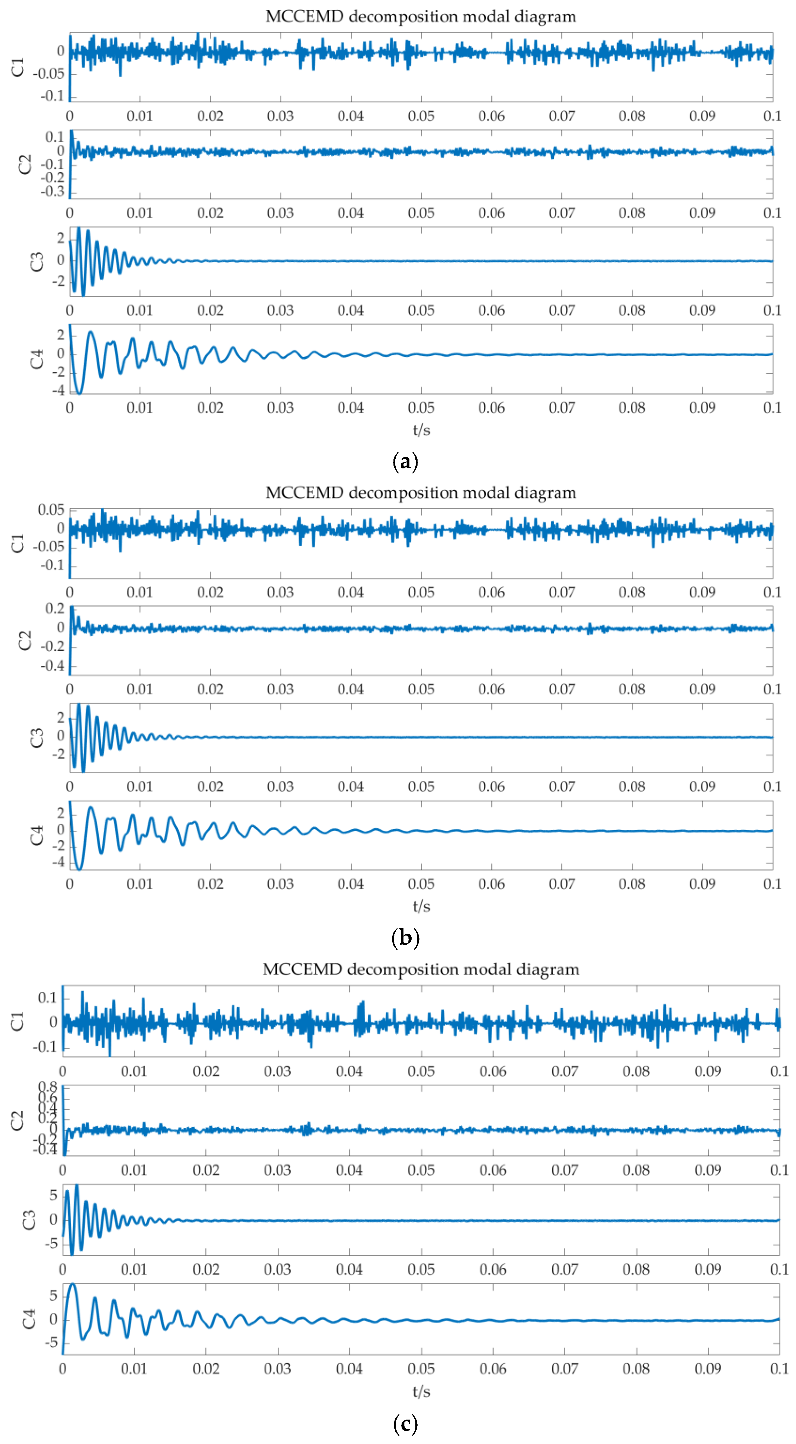
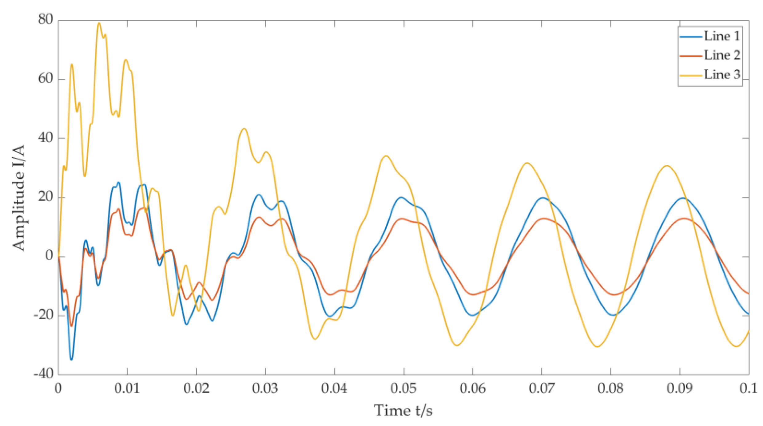
Under the conditions of a metal earthing fault, the zero-sequence current of the earthing fault occurred at a distance of fault bus L = 3 km, as shown in Figure 4. The modal function diagram obtained by the MCEEMD adaptive decomposition of the fault current is shown in Figure 5.
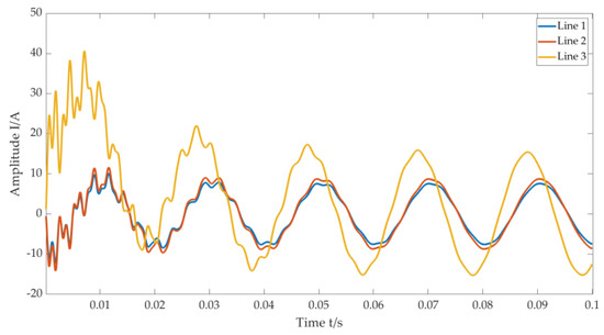
Figure 4.
Diagram of a resonant grounding system with a single-phase grounding fault.
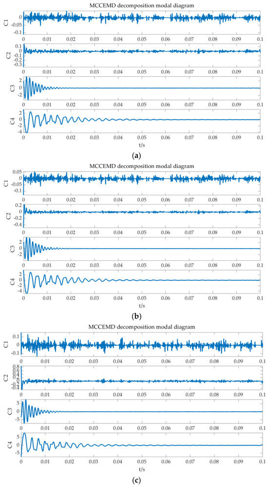
Figure 5.
MCCEMD breakdown diagram for each line. (a) MCCEMD breakdown diagram for Line 1; (b) MCCEMD breakdown diagram for Line 2; (c) MCCEMD breakdown diagram for Line 3.
It can be seen in Figure 4 that the amplitudes of Line 1 and Line 2 are close, while the amplitude of Line 3 has obvious fluctuations and is higher than that of Line 1 and Line 2; therefore, it was determined that Line 3 is the fault line.
(2) The entropy of the fault signal standardization multi-scale permutation is calculated, as shown in Table 1.

Table 1.
Standardized MPE value for the faulty line L = 3 km.
(3) Clustering simulation results analysis
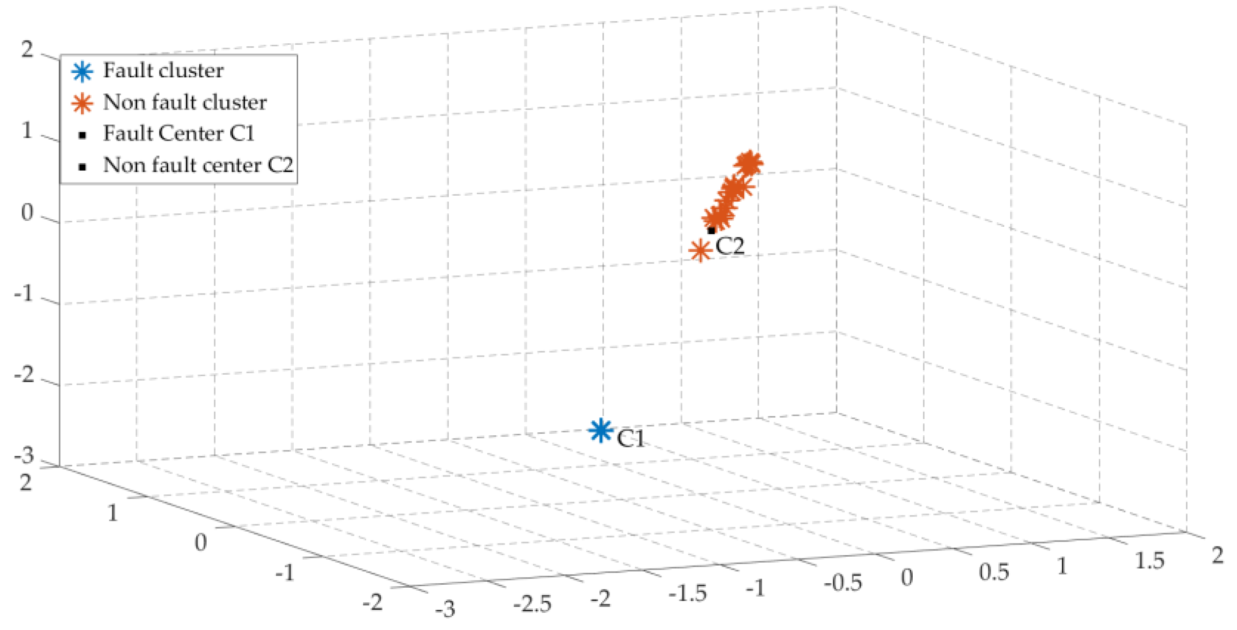
According to the calculation, the cluster centers of the fault line cluster and the non-fault line cluster shown in Figure 6 are C1 = (−1.476, −1.478, −1.475) and C2 = (0.157, 0.157, 0.157), respectively.

Figure 6.
Clustering analysis diagram of fault line L = 3 km.
The normalized multi-scale permutation entropy value of the fault line L = 6 km and its clustering analysis diagram are shown in Supplementary Table S1 and Supplementary Figure S1; the normalized multi-scale permutation entropy value and its clustering analysis diagram with the initial phase angle of , , are shown in Supplementary Table S2 and Supplementary Figure S2; the clustering analysis diagram under different fault distances and initial phase angles is shown in Supplementary Figure S3.
According to the analysis of Figure 6 above, upon the occurrence of a single-phase-to-ground fault in phase a of Line 3, the decomposed entropy matrix is classified by a k-means clustering algorithm. Finally, the fault line and non-fault line are clustered and identified using a three-dimensional Cartesian coordinate system to identify the fault line non-fault line under different fault distances and different initial phase angles.
4. Analysis of Single-Phase Grounding Fault in Resonant Grounding System Based on Actual Measurement Site
4.1. Fault Signal Line Selection Analysis of Real Test Site
Figure 7 below shows the plan of actual test site with six feeders. Lines 1, 2, and 3 are true overhead lines with no loads, respectively. Lines 4, 5, and 6 are impedance analog lines with circuit breakers; the three lines can be run either without loads or with loads and the terminals of Lines 4 and 5 are connected to a transformer which can directly carry out a bench simulation with a capacity of 315 kVA. All lines can obtain the zero-sequence current and phase current, recording data from each line in real time. There are many grounding modes and different grounding fault points at the neutral point of the test site; different grounding fault effects can be achieved by changing different grounding modes with switches. In the test field case, the no-load overhead lines, Line 1, Line 2, and Line 3 were used as the test object. Line 3 was set as the fault line. Line 1 had a length of 9 km. Line 2 and Line 3 had lengths of 6 km and 9 km, respectively.
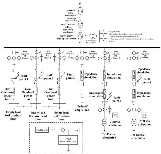
Figure 7.
Plane construction drawing of the test site.
According to the single-phase grounding fault simulation analysis of the actual test site shown in Figure 7, the extracted fault data were analyzed and processed and are shown in Figure 8.
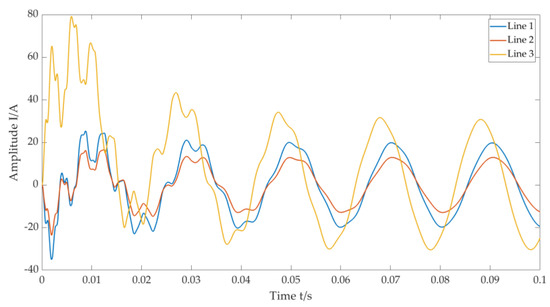
Figure 8.
Single-phase grounding fault line diagram of the actual test site.
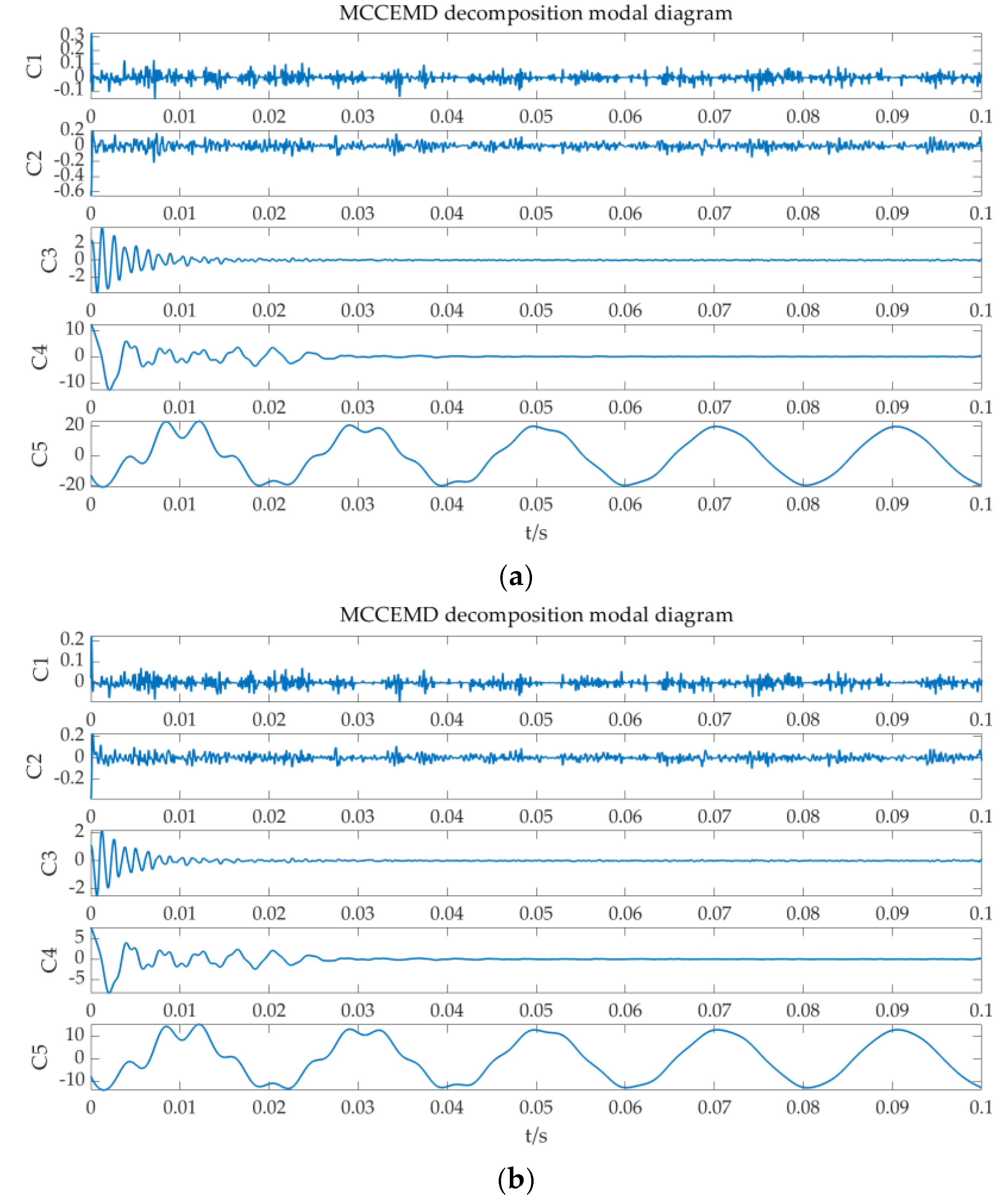
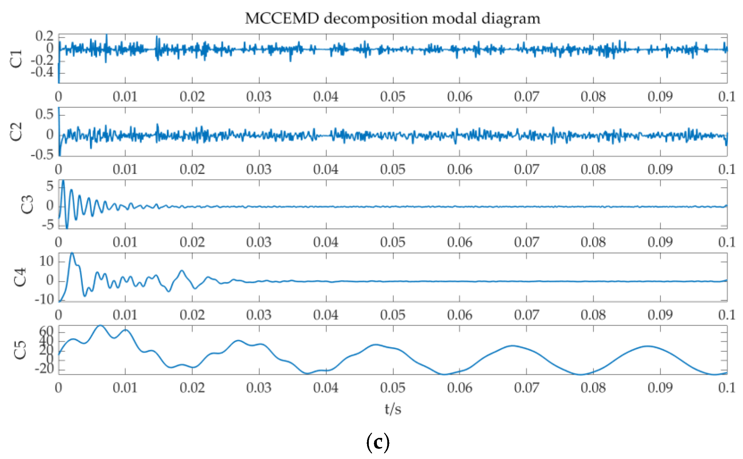
It can be seen from Figure 8 that the amplitudes of Line 1 and Line 2 are close, while the amplitude of Line 3 has obvious fluctuations and is higher than that of Line 1 and Line 2; therefore, Line 3 is identified as the fault line. The collected data are decomposed by the MCEEMD-MPE standardization algorithm, as shown in Figure 9. Then, the standardized entropy values are calculated, as shown in Table 2.
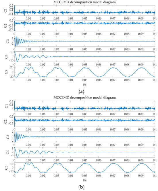
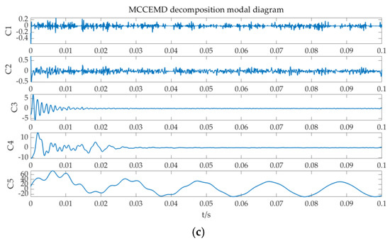
Figure 9.
Decomposition diagram of MCCEMD for each line: (a) decomposition diagram of MCCEMD of Line 1; (b) decomposition diagram of MCCEMD of Line 2; and (c) decomposition diagram of MCCEMD for Line 3.
Table 2.
Standardized MPE values for faulty line L = 4 km.
4.2. Cluster Analysis of True Type Test Site
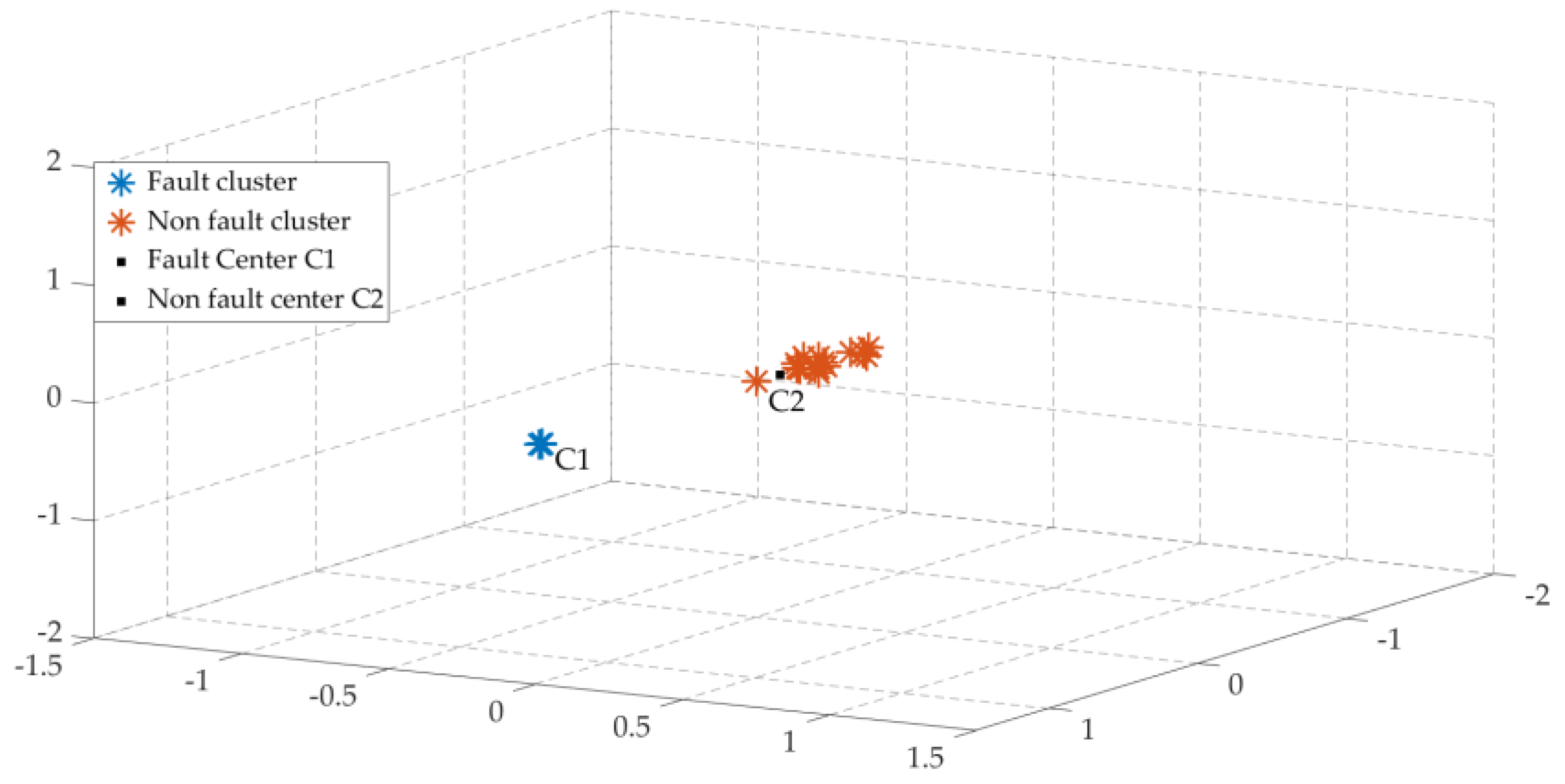
According to the calculation, the cluster centers of the fault line cluster and the non-fault line cluster shown in Figure 10 are C1 = (−1.49, −1.48, −1.48) and C2 = (0.003, 0.003, 0.003), respectively.
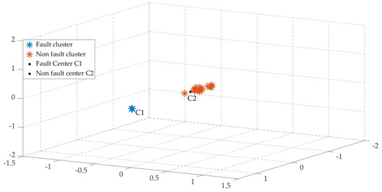
Figure 10.
Clustering analysis diagram of fault line L = 4 km.
The normalized multi-scale permutation entropy value of the fault line L = 7 km and its clustering analysis diagram are shown in Supplementary Table S3 and Supplementary Figure S4; the normalized multi-scale permutation entropy value and its clustering analysis diagram with the initial phase angle of , , are shown in Supplementary Table S4 and Supplementary Figure S5; the clustering analysis diagram under different fault distances and initial phase angles is shown in Supplementary Figure S6.
According to the analysis of Figure 8 above, upon the occurrence of a single-phase-to-ground fault in phase a of Line 3, the decomposed entropy matrix is classified by the k-means clustering algorithm. Finally, the fault line and non-fault line are clustered and identified using a three-dimensional Cartesian coordinate system to identify the fault line and non-fault line under different fault distances and different initial phase angles.
4.3. Method Comparison
To verify the effectiveness of the line selection algorithm introduced in this paper, the single-phase ground fault on the L1 line of an actual test case is taken as an example. The fault distance is set L = 4 km, and the fault resistance is, respectively, metallic grounding, 100 ω, 500 ω, 1000 ω, 2000 ω. The fault line selection used MCEEMD-MPE and k-means algorithms, EMD-MPE and k-means algorithms, EEMD-MPE and k-means algorithms, and HHT-MPE and k-means algorithms, respectively, as shown in Table 3.
Table 3.
Comparison of different algorithms for line identification.
From Table 3, it can be concluded that the EMD-MPE–k-means clustering algorithm and EEMD-MPE–k-means clustering algorithm cannot effectively identify fault lines and non-fault lines. The HHT-MPE–k-means clustering algorithm can see that the non-fault clusters are scattered widely, and the clustering effect is not obvious because of the close distance between the fault clusters and the non-fault clusters, which makes the fault clusters and the non-fault clusters overlap. However, the clustering algorithm of the MCEEMD-MPE–k-means algorithm used in this paper can distinguish fault lines from non-fault lines effectively. Therefore, the algorithm introduced in this paper demonstrates superiority over existing algorithms.
5. Conclusions
A fault line selection method based on a combination of MCEEMD-MPE normalization and the k-means clustering algorithm is proposed for the phase grounding fault problem of a resonant grounding system. First, the MCEEMD method was applied to the analysis of single-phase grounding fault signals in resonant grounding. The signals were decomposed into modal components with certain bandwidth frequencies, which avoids the mode-aliasing phenomenon and unnecessary ensemble averaging of the decomposed signals, providing an information-rich data source for subsequent fault recognition. Second, multi-scale permutation entropy was used to normalize the calculated entropy values to unify the characteristics of the fault signal for calculation and analysis. Third, the unified signal entropy value matrix was input into the k-means clustering algorithm to correctly identify the fault line and non-fault lines. The above method has a strong recognition effect on the fault line selection of resonant grounding systems with single-phase grounding faults. The recognition rate is 100%.
Supplementary Materials
The following supporting information can be downloaded at: https://www.mdpi.com/article/10.3390/pr13020475/s1, Figure S1: Clustering Analysis diagram of fault line L = 6 km; Figure S2: The cluster analysis diagram of different fault initial phase angle; Figure S3: Clustering Analysis diagram of different fault distance and initial phase angle; Figure S4: Clustering Analysis diagram of fault line L = 7 km; Figure S5: The cluster analysis diagram of different fault initial phase angle; Figure S6: Clustering Analysis diagram of different fault distance and initial phase angle; Table S1: The normalized MPE value of the faulty line L = 6 km; Table S2. Standardized MPE values for different initial phase angles. Table S3: Standardized MPE values for faulty line L = 7 km. Table S4: Standardized MPE values for different initial phase angles.
Author Contributions
Y.L. proposed the initial concept of the article and completed the logical outline and parameter preparation of the article. C.L. completed the plan description, the article, and constructed the system model. W.C. provided comprehensive guidance and review on the logic of the entire article. All authors have read and agreed to the published version of the manuscript.
Funding
This work was supported in part by the Academic Degrees and Graduate Education Reform Project of Henan Province (No. 2021SJGLX078Y).
Data Availability Statement
The data that support the findings of this study are available from the corresponding author upon reasonable request.
Conflicts of Interest
Author Chen Li was employed by the Henan High-speed Railway Co., Ltd. Author Wensi Cao was employed by the North China Institute of Water Conservancy and Hydroelectric Power. The remaining authors declare that the research was conducted in the absence of any commercial or financial relationships that could be construed as a potential conflict of interest.
References
- Li, L.; Gao, H.; Yuan, T.; Peng, F. A method for single-phase ground fault detection and location in distribution network based on zeroquence transient variable. Autom. Electr. Power Syst. 2025, 1–13. Available online: http://kns.cnki.net/kcms/detail/32.1180.tp.20250113.1450.005.html (accessed on 5 February 2025).
- Wang, W.; Zhang, P.; Gao, Q.; Li, Q. Single-phase ground fault location based on transient information fusion. J. Tianjin Univ. Technol. 2025, 1–9. [Google Scholar]
- Wang, Y.; Liu, J.; Zhang, Z.; Zheng, T.; Ren, S.; Chen, J. A faulty line detection method for single phase-to-ground fault in resonant grounding system with CTs reversely connected. Int. J. Electr. Power Energy Syst. 2023, 147, 108873. [Google Scholar] [CrossRef]
- Zhang, F.; Xue, Y.; Xu, B. A method for calculating the residual current at the fault point of a resonant system based on signal injection. Power Syst. Prot. Control 2023, 51, 132–138. [Google Scholar] [CrossRef]
- Wang, W. Research on Identification Method of High Impedance Grounding Fault in Distribution Network. Master’s thesis, Nanjing University of Posts and Tele, Nanjing, China, 2023. [Google Scholar]
- Ou, Y.; Shu, Q. A method for fault line selection and section location of resonant grounding system based on SOM and Kans clustering. Electr. Technol. 2023, 24, 23–30. [Google Scholar]
- Wu, J.; Zheng, M.; Wang, X.; Li, H.; Luo, H. A method for single-phase ground fault line selection in resonant grounding based on transient zero-sequence admittance value. South. Power Grid Technol. 2024, 18, 58–66. [Google Scholar]
- Yang, C.; Cai, B.; Liu, Y.; Kong, X.; Shao, X.; Shao, H. Intelligent full-stage stable fault diagnosis method for subsea production system. Ocean Eng. 2024, 312, 119309. [Google Scholar] [CrossRef]
- Yang, C.; Cai, B.; Wu, Q.; Wang, C.; Ge, W.; Hu, Z.; Zhu, W.; Zhang, L.; Wang, L. Digital twin-driven fault diagnosis method for composite faults by combining virtual and real data. J. Ind. Inf. Integr. 2023, 33, 100469. [Google Scholar] [CrossRef]
- Yang, C.; Cai, B.; Zhang, R.; Zou, Z.; Kong, X.; Shao, X.; Liu, Y.; Shao, H.; Khan, J.A. Cross-validation enhanced digital twin driven fault diagnosis methodology for minor faults of subsea production control system. Mech. Syst. Signal Process. 2023, 204, 110813. [Google Scholar] [CrossRef]
- Chen, B.; Sun, Y.; Song, X.; Wang, B. Regionalized fault line in distribution networks based on an improved SSA-VMD and multi-scale fuzzy entropy. Electr. Eng. 2023, 105, 4399–4408. [Google Scholar] [CrossRef]
- Chen, Y.; Liu, F.; Zhou, T.; Li, P.; Gan, P.; Hou, M. Research on Single-phase Grounding Fault Line Selection Based on VMD Method. J. Phys. Conf. Ser. 2023, 2650, 012043. [Google Scholar] [CrossRef]
- Jia, M. Ground fault location of long-distance UHV transmission line based on EMD decomposition algorithm. Electr. Eng. Technol. 2024, 3, 177–179+201. [Google Scholar]
- Li, Y.; Fan, M.; Zhu, Y.; Liu, Z. Research on fault diagnosis of conveyor belt gearbox based on EEMD and SVM. Electr. Mech. Inf. 2024, 24, 74–78. [Google Scholar]
- Ding, Y.; Chen, Z.; Zhang, H.; Wang, X.; Guo, Y. A short-term wind power prediction model based on CEEMD and WOA-KELM. Renew. Energy 2022, 189, 188–198. [Google Scholar] [CrossRef]
- Zhang, Y.; Li, Z.; Wang, J.; Zhang, T.; Zhang, Y. Detection of flat-bottom holes in composite materials using multi-dimensional complementary ensemble empirical mode decomposition algorithm. J. Instrum. 2023, 18, T11002. [Google Scholar] [CrossRef]
- Liu, S.; He, B.; Chen, Q.; Lang, X.; Zhang, Y. Median Complementary Ensemble Empirical Mode Decomposition and its application to time-frequency analysis of industrial oscillations. In Proceedings of the 2021 40th Chinese Control Conference (CCC), Shanghai, China, 26–28 July 2021; IEEE: Piscataway, NJ, USA, 2021; pp. 2999–3004. [Google Scholar]
- Liu, S.; Lang, X.; Zhang, Y.; Li, P.; Xie, L.; Su, H. An Automated Diagnostic Framework for Multiple Oscillations With Median Complementary EEMD. IEEE Trans. Control Syst. Technol. 2023, 32, 919–933. [Google Scholar] [CrossRef]
- Hou, S.; Guo, W. Optimal denoising and feature extraction methods using modified CEEMD combined with duffing system and their applications in fault line selection of non-solid-earthed network. Symmetry 2020, 12, 536. [Google Scholar] [CrossRef]
- Hong, Y.; Xu, L.; Su, J.; Wang, H.; Li, M. Short-term power load forecasting based on BFVMD-PE and deep learning. Control Eng. 2025, 1–11. [Google Scholar] [CrossRef]
- Liu, F.; Zhang, L.; Pang, B.; Liang, C.; Yao, Y. A noise reduction method and its application for the vibration signal of the guide based on CEEMDAN and MPE. J. Zhengzhou Univ. (Eng. Ed.) 2022, 43, 91–97. [Google Scholar]
- Zhang, Y.; Li, Y. Fault diagnosis of rolling bearings based on multi-scale permutation entropy and IWOA-SVM. Electron. Technol. 2023, 46, 29–34. [Google Scholar]
- Sun, Y.; Cao, Y.; Li, P.; Li, X. A for fault diagnosis of turnout machine based on multi-scale permutation en-tropy and 2nd order feature selection by wavelet packet decomposition. China Railw. Sci. 2023, 44, 178–188. [Google Scholar]
- Ma, T.; Li, W.; Chen, J.; Lai, Y.; Yang, Z. Identification of short wavelength rail corrugation in subway based on CEEMD-MPE algorithm. Noise Vib. Control 2023, 43, 120–126+153. [Google Scholar]
- Granat, R.; Donnellan, A.; Heflin, M.; Lyzenga, G.; Glasscoe, M.; Parker, J.; Pierce, M.; Wang, J.; Rundle, J.; Ludwig, L.G. Clustering analysis methods for GNSS observations: A data-driven approach to identifying California's major faults. Earth Space Sci. 2021, 8, e2021EA001680. [Google Scholar] [CrossRef]
- Gao, W.; Xi, D.; Zheng, L. Correlation and K-means clustering based small current ground fault line selection algorithm. J. Phys. Conf. Ser. 2023, 2598, 012010. [Google Scholar] [CrossRef]
- You, Z.; Yuan, X.; Min, R.; Li, W. Clustering analysis of shield machine main bearings based on improved k-means. Mechatronics 2022, 28, 17–21. [Google Scholar]
- Gu, Z.; Lin, Y. Fault diagnosis of rolling bearings based on improved LMD and comprehensive feature indicators. J. Hefei Univ. Technol. (Nat. Sci. Ed.) 2021, 44, 145–150+181. [Google Scholar]
- Tao, R.; Lu, T.; Zhou, Z. A method for extracting GNSS coordinate time series signals based on the combination of WT and MPE. J. Surv. Mapp. Sci. Technol. 2024, 40, 446–452. [Google Scholar]
- Ding, X.; Zhang, Y. Gearbox feature extraction and fault diagnosis based on ICEEMDAN-MPE-RF and SVM. Locomot. Electr. Transm. 2023, 1, 42–50. [Google Scholar]
- Han, D.; Guo, X.; Shi, P. An intelligentfault diagnosis method of variable condition gearbox basedon improved DBN combined with WPEE and MPE. IEEE Access 2020, 8, 131299–131309. [Google Scholar] [CrossRef]
- Xu, H.; Pan, C. A rolling bearing fault diagnosis method based on ICEEMDAN-MPE and GWO-SVM. J. Natl. Def. Transp. Eng. Technol. 2024, 22, 33–37+96. [Google Scholar]
- Starovoitov, V.V.; Golub, Y.I. Data normalization in machine learning. Informatics 2021, 18, 83–96. [Google Scholar] [CrossRef]
- Barstuğan, M.; Arabacı, H. Rotor fault characterization study by considering normalization analysis, feature extraction, and a multi-class classifier. Eng. Res. Express 2024, 6, 025304. [Google Scholar] [CrossRef]
- Wu, Z.; Wu, J.; Wu, H. Clustering analysis of bank and real estate stock price fluctuations based on DT-K-means model. Financ. Financ. 2022, 5, 37–44. [Google Scholar]
- Xu, Y.; Tian, S.; Yang, Q. Fault line selection of resonant grounding system based on comprehensive high and low frequency components. Proc. Chin. Soc. Electr. Eng. 2021, 33, 1–9. [Google Scholar]

Disclaimer/Publisher’s Note: The statements, opinions and data contained in all publications are solely those of the individual author(s) and contributor(s) and not of MDPI and/or the editor(s). MDPI and/or the editor(s) disclaim responsibility for any injury to people or property resulting from any ideas, methods, instructions or products referred to in the content. |
© 2025 by the authors. Licensee MDPI, Basel, Switzerland. This article is an open access article distributed under the terms and conditions of the Creative Commons Attribution (CC BY) license (https://creativecommons.org/licenses/by/4.0/).