Abstract
The compressor is a critical component of cryogenic separation industrial systems, and its reliable operation is essential for the stable functioning of the entire system. Existing research focuses on predicting compressor conditions using experimental or simulation data, often neglecting analysis based on actual industrial data. To address this gap, this paper presents an innovative prediction model for compressor data utilizing an LSTM–self-attention mechanism, specifically designed for real industrial systems. The proposed model combines the sequential learning capabilities of LSTM with the dynamic feature extraction strengths of self-attention, enabling highly accurate predictions by enhancing sensitivity to critical data features. The actual vibration data from a compressor spanning 12 months are analyzed and compared. The results demonstrate that the proposed model reduces prediction error by in MSE and in RMSE compared to SVR. These findings highlight the model’s potential for real-time monitoring and early fault detection, providing a robust theoretical foundation for condition-based analysis and preventive maintenance in industrial compressor applications.
1. Introduction
Compressors are critical components in various industrial applications, including petrochemical, energy, and manufacturing sectors, where their operational stability and efficiency are essential to ensure uninterrupted production [1,2,3]. As a key element in process industries [4,5,6], compressors play an indispensable role in maintaining the continuous flow of materials and energy throughout complex industrial systems. Due to complex working conditions and prolonged operation, compressors are prone to faults and performance degradation, which can lead to significant downtime and maintenance costs. Predicting compressor behavior, particularly through time series data such as vibration signals, has become an essential task in modern predictive maintenance strategies. This not only reduces unexpected failures but also optimizes maintenance schedules, enhancing overall operational efficiency. Traditional methods for fault diagnosis and prediction have limitations when dealing with large-scale, high-dimensional, and noisy data. To address these challenges, machine learning techniques, especially deep learning models, have gained increasing attention for their ability to model complex, nonlinear relationships in time series data.
Researchers have conducted valuable analysis on the condition monitoring of mechanical equipment based on intelligent models [7,8,9,10]. Recent advancements in compressor condition monitoring and predictive analysis have utilized various models to enhance fault detection and prediction accuracy. Ghorbanian and Gholamrezaei [11] pioneered the artificial neural network to predict the compressor performance via experimental data to achieve a good predicted result. Wang et al. [12] developed a novel correlation factor with a genetic algorithm to accurately predict the low speed variation trends of the compressor performance. Zhang et al. [13] established a new less-correlation selection method to predict centrifugal compressors that is superior to the conventional loss correlation set. Samuel et al. [14] utilized a machine learning tool to predict compressor stalls, achieving a prediction window of 5–20 ms prior to stall occurrences. Wu et al. [15] applied support vector regression (SVR) and Gaussian process regression models to train a surrogate model to predict the overall performance of the compressor. The experimental studies showed that the predicted error can be well reduced with the proposed method. Liu et al. [16] proposed intelligent fault diagnosis for compressors combining local mean decomposition and a stack-denoising autoencoder. Wu et al. [17] employed an artificial intelligence-based neural network to forecast the electrical load profile. Tian et al. [18] introduced a different term for the maximum mean discrepancy into a deep convolutional autoencoder to effectively enhance the prediction performance while pursing efficiency. Experimental results demonstrated that the prediction accuracy was higher than that of other mainstream models. Zhong et al. [19] predicted the performance of a compressor using a support vector machine (SVM) and genetic algorithm (GA) to optimize the parameters. The proposed SVM-GA method has a better generalization and more accurate predict performance than other methods. Jeong et al. [20] developed an artificial neural network and a simplified reduced-order system model to predict the performance of a compressor. The proposed model was tested through an experimental study to demonstrate its effectiveness. Peng et al. [21] proposed an attention and multi-scale convolutional neural networks to extract features and utilized LSTM to predict the remaining useful life of the compressor. Their simulation dataset demonstrated that their proposed method can reduce the prediction error.
Despite the progress made in compressor condition prediction through a series of studies in the literature, existing research has primarily focused on simulated and experimental data for compressor monitoring. Currently, there is a lack of predictive analysis of compressors in real-world process industries. Therefore, it is essential to develop data-driven intelligent prediction models to achieve accurate condition forecasting for actual compressors. This advancement would reduce operational risks in industrial systems and provide a basis for preventive maintenance.
Toward the above problems, this paper proposes an LSTM- and self-attention-based model to predict the monitored data of a compressor from an actual petroleum system. The proposed model fully combines the advantages of LSTM and a self-attention mechanism to achieve accurate prediction results. A case study with monitored data of a compressor was conducted to demonstrate the effectiveness of the proposed model. The accurate and intelligent prediction results obtained show that the proposed model has the capability to significantly reduce the operational risk of the compressor.
2. Research Methodology
2.1. Basic Theory
2.1.1. LSTM
LSTM (long short-term memory) is a variant of an RNN (recurrent neural network) that excels at capturing long-term dependencies and is well suited for sequence prediction tasks. Standard RNNs, when dealing with long sequences, encounter issues such as vanishing or exploding gradients as the time steps increase, making it difficult for the model to capture dependencies over long time spans. LSTM alleviates these problems by introducing special memory cells and gating mechanisms, allowing it to effectively handle these challenges.
The core of LSTM lies in its three gates and a memory cell (cell state). These gates help the model manage the flow of information by selectively forgetting, discarding, or retaining information. The LSTM structure is depicted in Figure 1.
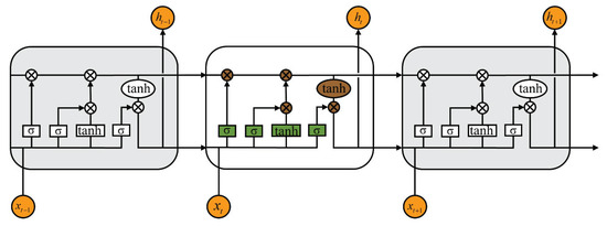
Figure 1.
LSTM structure.
The diagram below illustrates the internal structure of the LSTM network, which includes three major gate components:
- 1.
- Forget gate:The forget gate determines whether the information from the previous time step should be retained or discarded. Based on the current time step input and the previous hidden state, the forget gate outputs a value between 0 and 1, which dictates how much of the past information should be forgotten. A value closer to 0 means that more information will be discarded, while a value closer to 1 indicates that more information will be retained. This mechanism allows the LSTM to selectively forget irrelevant information and focus on relevant patterns. The mathematical expression of the forget gate can be expressed as follows:where is the output of the forget gate, is the hidden state from the previous time step, is the input at time t, is the weight matrix, is the bias matrix, and denotes the sigmoid activation function, which can be expressed aswhere x represents any input variable.
- 2.
- Input gate:The input gate quantifies the importance of the new information carried by the input and selectively records it in the memory cell. First, a “how much to retain” coefficient is calculated using the sigmoid function, and then a candidate memory state is generated using the tanh function. The two are multiplied to obtain the new information to be added to the memory cell. This process can be divided into two steps: First, how much of the new information to keep is determined via the sigmoid gate, as shown below:where represents the output of the input gate, and and are the weight and bias matrices of the input gate, respectively. Second, the candidate memory content is generated based on the current input and previous hidden state through the tanh function:where represents the candidate memory state, and and are the weight and bias matrices, respectively.
- 3.
- Output gate:
The output gate determines the hidden state output for the current time step. In combining the current memory cell state with the output gate’s results, the model generates the hidden state for the next time step, which can be expressed as
where is the output of the output gate, and and are the weight and bias matrices of the output gate.
These three gates control the flow of information into and out of the LSTM cell. An LSTM unit (which includes these three gates and one LSTM cell) can be viewed as a layer of neurons in a traditional feedforward neural network. Each neuron in the LSTM has both a hidden state and a current cell state, enabling it to manage and retain information over time, which is essential for capturing temporal dependencies in sequential data. For each time step, the memory cell is updated based on the output of the forget gate and the new information, as shown in the following equation:
2.1.2. Self-Attention Mechanism
Self-attention is a powerful mechanism in deep learning, primarily used to capture global dependencies in sequence data. The core idea of the self-attention mechanism is that for each element in the input sequence (such as a word or time step), it calculates its relevance (or attention weights) with respect to all other elements in the sequence. This mechanism allows the model to weigh the importance of different elements dynamically. Self-attention is widely applied in the Transformer architecture, which has become the foundation for many modern natural language processing models.
For each input element, three vectors are generated through different linear transformations: the query vector , the key vector , and the value vector . These vectors serve the following purposes:
- Query (Q): Used to match with the keys of other elements to identify which elements are related to the current one.
- Key (K): Paired with the query to measure the similarity between different elements.
- Value (V): Once matching is complete, it determines how the information of this element will influence the final output based on the similarity weights.
The process can be mathematically expressed by the following equation:
where is the dimensionality of the key vector, and the function is
where is the ith element of the input vector . The softmax function converts a vector of values into a probability distribution, where the sum of all probabilities equals 1. It is commonly used to normalize the attention scores in the self-attention mechanism.
2.2. The Proposed Model
In considering that LSTM tends to suffer from attenuation and loss of long-distance dependencies when handling longer sequences, the introduction of the self-attention mechanism addresses this issue. By calculating the similarity between all positions in the sequence, self-attention enables the weighted integration of global information, thereby directly capturing long-distance dependencies. This effectively resolves the problem of dependency decay that LSTM faces in long sequences.
The proposed self-attention–LSTM model consists of four major procedures, namely forward propagation, loss function construction, backward propagation, and parameter update, as shown in Figure 2.
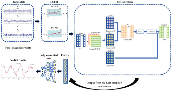
Figure 2.
LSTM and self-attention structure.
2.2.1. Forward Propagation
Regarding the time series-monitored data from the compressor, , as the input to the LSTM, the hidden state and the cell state are calculated at each time step, which can be expressed as
The hidden state at each time step forms the sequence of outputs from the LSTM, denoted as . These hidden states capture the temporal dependencies within the input sequence.
Subsequently, the self-attention mechanism is applied to the hidden states H, by projecting them into three matrices: query (Q), key (K), and value (V). This process can be mathematically represented as
where , , and are learned weight matrices, and Q, K, and V represent the query, key, and value matrices, respectively.
The attention scores between time steps are computed by taking the dot product of the query and key matrices, scaled by the square root of the dimensionality of the key vectors:
where is the dimensionality of the key vectors. The softmax function ensures that the attention weights sum to 1, allowing the model to focus on the most relevant parts of the sequence.
The output of the self-attention layer is a context-aware representation of the input sequence, capturing dependencies across all time steps. This context-enhanced representation, combined with the temporal features extracted by the LSTM, is then used for the final prediction task. Typically, the final hidden state from the LSTM or the output of the attention layer is passed through a fully connected layer to produce the output, denoted as
where represents the final output of the combined LSTM and attention mechanism, and FC is the fully connected layer used for the final prediction.
2.2.2. Loss Function
A loss function is constructed to measure the error between the output of the proposed model and the monitored data. This loss function will guide the model’s learning process on the compressor-monitoring data, thereby improving prediction accuracy. To this end, a mean squared error (MSE) function is established, which can be expressed as follows:
where denotes the calculated value of the loss function, N is the number of monitored data points, represents the predicted value from the model output for the ith sample, and indicates the corresponding ith value from the monitored data. This loss function effectively captures the average squared differences between predicted and actual values, allowing for a quantifiable assessment of the model’s performance. By minimizing this loss during training, the model can learn to make more accurate predictions based on the observed compressor-monitoring data.
2.2.3. Backpropagation
The backpropagation process in LSTM generally involves the following steps:
- 1.
- Gradient of loss with respect to hidden statePerform backpropagation through time from the last time step T to the first time step 1. For each time step, calculate the gradient of the output, forget, and input gates:where represents the gradient at the current time step.
- 2.
- Updating cell stateThe cell sate can be updated based on the following equation:
- 3.
- Gradient of the weights and biases of LSTMThe gradients for the weight and bias for each time step can be determined using the chain rule:Following the above equations, each gradient expression uses summation over time steps t to accumulate the contributions from all time steps
- 4.
- Gradients of the self-attentionThe gradient of matrices Q, K, and V in self-attention can be calculated based on the following equation:
These gradient equations can be used during optimization to update the weight parameters of the self-attention mechanism.
2.2.4. Parameter Updating
To optimize the parameters of an LSTM combined with a self-attention mechanism, the update rules for the parameters typically follow the equations below:
where denotes the , , , of the LSTM (for the forget gate, input gate, cell state, and output gate), biases (, , , and ) and parameters of self-attention (, , and ), and denotes the learning rate.
These update rules ensure that the model’s parameters are adjusted in the direction that minimizes the loss function. Each gradient is computed during backpropagation, capturing how changes in the parameters affect the loss. With these formulas, an LSTM model with a self-attention mechanism can be effectively trained. Once the parameters finish training, the model is evaluated on validation or test datasets to assess its performance.
3. Results
3.1. Industrial System Introduction
The analyzed compressor was a part of a natural gas comprehensive utilization project, featuring core units of natural gas liquefaction. The project was built in Xinjiang province, China, and a photograph (Figure 3) is shown below.
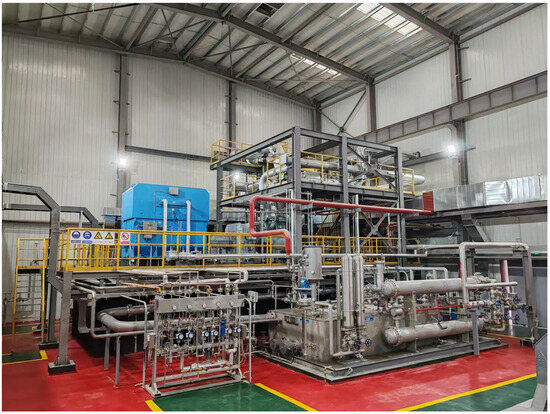
Figure 3.
A photograph of the compressor.
A vibration sensor was mounted on the housing of the compressor to monitor vibration data. The sensor was an eddy current vibration displacement sensor, model Y823X1100VD9061, compliant with the FB65114.2 standard. The total probe length was 1 m. The sensor was installed as shown in the Figure 4 below.
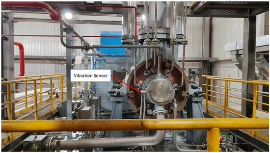
Figure 4.
The position of the installed sensor.
3.2. Data Introduction
The vibration data were collected through the sensor, with a time duration of one year, namely from August, 2023 to September, 2024. The monitored data are plotted in Figure 5, Figure 6, Figure 7, Figure 8, Figure 9, Figure 10, Figure 11, Figure 12, Figure 13, Figure 14, Figure 15 and Figure 16.
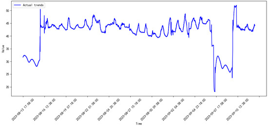
Figure 5.
Monitored data of the compressor from 2023.8 to 2023.9.
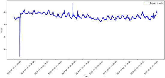
Figure 6.
Monitored data of the compressor from 2023.9 to 2023.10.
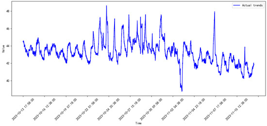
Figure 7.
Monitored data of the compressor from 2023.10 to 2023.11.
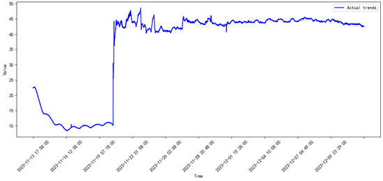
Figure 8.
Monitored data of the compressor from 2023.11 to 2023.12.
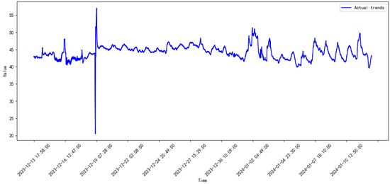
Figure 9.
Monitored data of the compressor from 2023.12 to 2024.1.
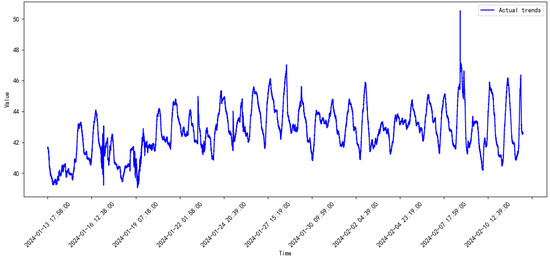
Figure 10.
Monitored data of the compressor from 2024.1 to 2024.2.
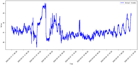
Figure 11.
Monitored data of the compressor from 2024.2 to 2024.3.
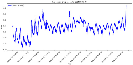
Figure 12.
Monitored data of the compressor from 2024.3 to 2024.4.
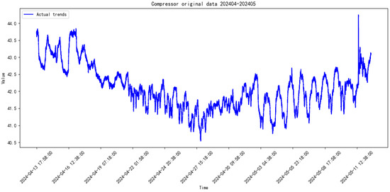
Figure 13.
Monitored data of the compressor from 2024.4 to 2024.5.
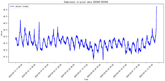
Figure 14.
Monitored data of the compressor from 2024.5 to 2024.6.
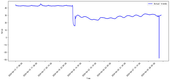
Figure 15.
Monitored data of the compressor from 2024.6 to 2024.7.
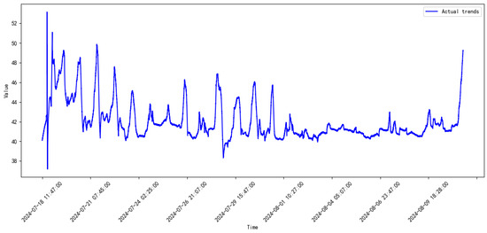
Figure 16.
Monitored data of the compressor from 2024.7 to 2024.8.
In order to validate the effectiveness of the proposed model, the monitored data were split into training and testing sets: 90% data points were selected for the training set, and the remaining points, for the testing set. The prediction error was calculated in terms of two indicators, namely the mean sqaure error (MSE) and root mean square error (RMSE).
3.3. Comparative Study
The effectiveness of the proposed model and the support vector regression (SVR) model was analyzed in this study. The models were implemented using Python V3.7 and executed on a 64-bit Windows 10 system with an i7-10875H processor. The parameters of the comparative models are outlined in Table 1.

Table 1.
Model’s parameter settings.
Following the model parameters listed above, for the vibration data of each month, 90% of data were for training, and 10% for testing. The prediction results of the proposed model are shown in Figure 17, Figure 18, Figure 19, Figure 20, Figure 21, Figure 22, Figure 23, Figure 24, Figure 25, Figure 26, Figure 27 and Figure 28.
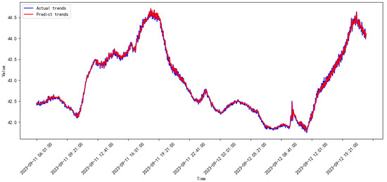
Figure 17.
Prediction results of the proposed model from 2023.08 to 2023.09.
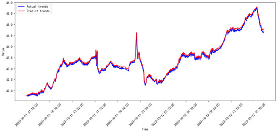
Figure 18.
Prediction results of the proposed model from 2023.09 to 2023.10.
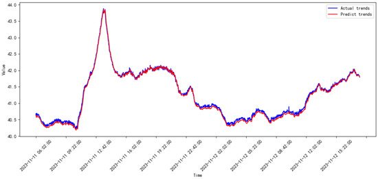
Figure 19.
Prediction results of the proposed model from 2023.10 to 2023.11.
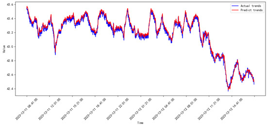
Figure 20.
Prediction results of the proposed model from 2023.11 to 2023.12.
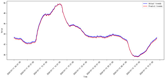
Figure 21.
Prediction results of the proposed model from 2023.12 to 2024.01.
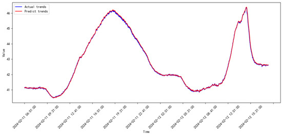
Figure 22.
Prediction results of the proposed model from 2024.01 to 2024.02.
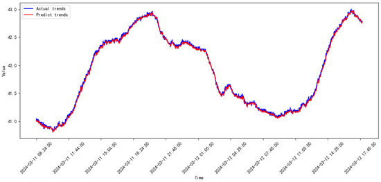
Figure 23.
Prediction results of the proposed model from 2024.02 to 2024.03.
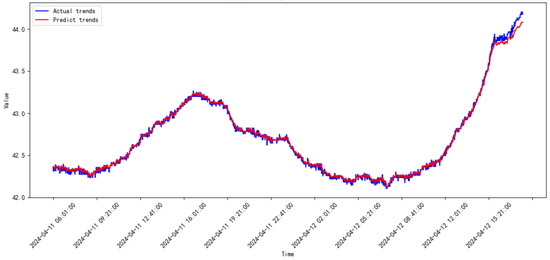
Figure 24.
Prediction results of the proposed model from 2024.03 to 2024.04.
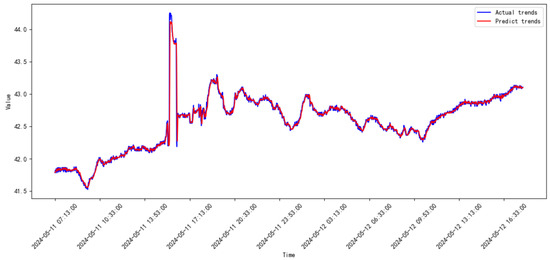
Figure 25.
Prediction results of the proposed model from 2024.04 to 2024.05.
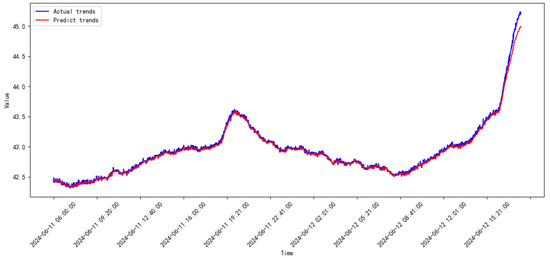
Figure 26.
Prediction results of the proposed model from 2024.05 to 2024.06.
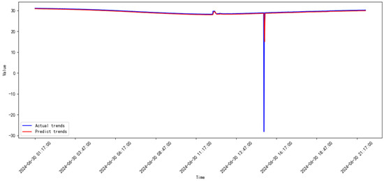
Figure 27.
Prediction results of the proposed model from 2024.06 to 2024.07.
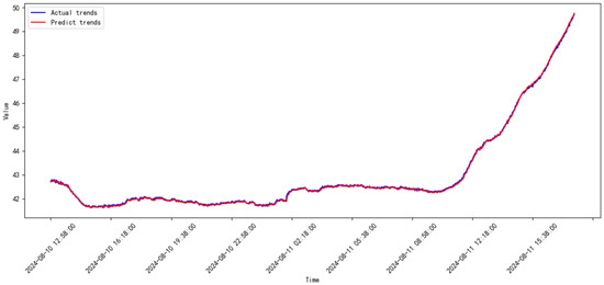
Figure 28.
Prediction results of the proposed model from 2024.07 to 2024.08.
The legends of the ‘predict’ and ‘actual’ trends in Figure 17, Figure 18, Figure 19, Figure 20, Figure 21, Figure 22, Figure 23, Figure 24, Figure 25, Figure 26, Figure 27 and Figure 28 are the predict results and actual data waveforms of the proposed model, respectively. Comparatively, the prediction results of the SVR for each month of the compressor’s vibration data are shown in Figure 29, Figure 30, Figure 31, Figure 32, Figure 33, Figure 34, Figure 35, Figure 36, Figure 37, Figure 38 and Figure 39.
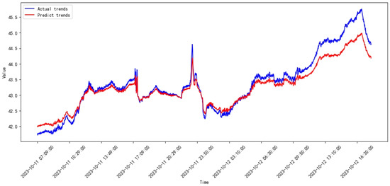
Figure 29.
Prediction results of SVR from 2023.09 to 2023.10.
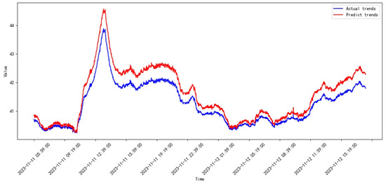
Figure 30.
Prediction results of SVR from 2023.10 to 2023.11.
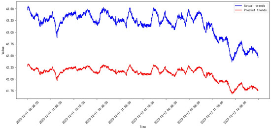
Figure 31.
Prediction results of SVR from 2023.11 to 2023.12.
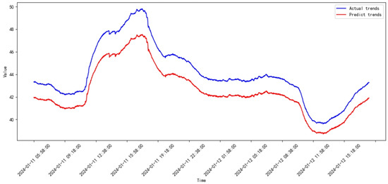
Figure 32.
Prediction results of SVR from 2023.12 to 2024.01.
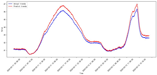
Figure 33.
Prediction results of SVR from 2024.01 to 2024.02.
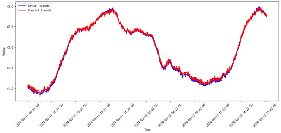
Figure 34.
Prediction results of SVR from 2024.02 to 2024.03.
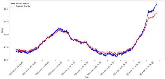
Figure 35.
Prediction results of SVR from 2024.03 to 2024.04.
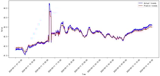
Figure 36.
Prediction results of SVR from 2024.04 to 2024.05.
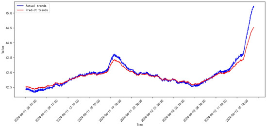
Figure 37.
Prediction results of SVR from 2024.05 to 2024.06.
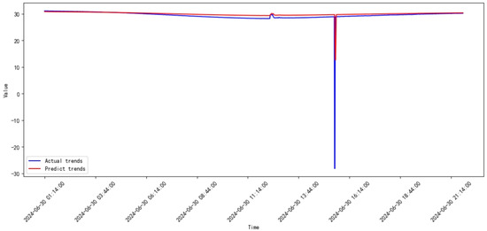
Figure 38.
Prediction results of SVR from 2024.06 to 2024.07.
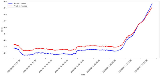
Figure 39.
Prediction results of SVR from 2024.07 to 2024.08.
The predicted errors calculated using the MSE and RMSE for each month are listed in Table 2.
Table 2.
Comparative results of the models.
3.4. Discussion
According to the prediction results in Figure 17, Figure 18, Figure 19, Figure 20, Figure 21, Figure 22, Figure 23, Figure 24, Figure 25, Figure 26, Figure 27, Figure 28, Figure 29, Figure 30, Figure 31, Figure 32, Figure 33, Figure 34, Figure 35, Figure 36, Figure 37, Figure 38 and Figure 39 and the errors listed in Table 2, the prediction trends of the proposed model are more accurate, and the errors are consistently smaller than those of SVR for every month. The ranges of the MSE and RMSE for the proposed mode are and , respectively. On the other hand, the ranges of the MSE and RMSE for SVR are and , respectively.
Additionally, the average values of the MSE and RMSE for the proposed model are 0.4446475 and 0.3067075, respectively. In contrast, the average values of the MSE and RMSE for SVR are 0.48297475 and 0.6158775, respectively. Consequently, the prediction error reductions achieved by the proposed model are approximately on the MSE and on the RMSE compared to SVR. These results demonstrate that the proposed model significantly outperforms SVR, showcasing its potential to achieve highly accurate predictions for compressor-monitored data.
4. Conclusions
This paper introduces a novel compressor data prediction model based on an LSTM–self-attention mechanism designed to analyze actual vibration data from a compressor. The proposed model effectively combines the sequential learning capability of LSTM with the adaptive weighting and feature extraction strengths of self-attention, enabling precise data prediction. Theoretical analysis of the model training process was conducted in detail. Actual vibration data spanning 12 months were analyzed and compared. The results show that the proposed model reduces the prediction error by for the MSE and for the RMSE relative to SVR, offering a valuable theoretical foundation for condition-based analysis and proactive maintenance strategies within industrial applications.
Author Contributions
Conceptualization, L.P., L.Z., J.L. and L.Q.; methodology, L.P., L.Z. and J.L.; software, L.P., L.Z. and J.L.; validation, L.P., L.Z., J.L. and L.Q.; formal analysis, L.P.; investigation, L.P., L.Z., J.L. and L.Q.; resources, L.P.; data curation, L.P., L.Z., J.L. and L.Q.; writing—original draft preparation, L.P., L.Z., J.L. and L.Q.; writing—review and editing, L.P., L.Z., J.L. and L.Q.; visualization, L.P., L.P., L.Z., J.L. and L.Q.; supervision, L.P., L.Z., J.L. and L.Q. All authors have read and agreed to the published version of the manuscript.
Funding
This research received no external funding.
Data Availability Statement
The data presented in this study are available on request from the corresponding author.
Conflicts of Interest
Author Liming Pu is employed by the China Petroleum Engineering & Construction Corporation Southwest Company. The remaining authors declare that the research was conducted in the absence of any commercial or financial relationships that could be construed as a potential conflict of interest.
Abbreviations
The following abbreviations are used in this manuscript:
| LSTM | Long short-term memory; |
| SVR | Support vector regression; |
| RNN | Recurrent neural network; |
| DL | Deep learning. |
References
- Romanssini, M.; de Aguirre, P.C.C.; Compassi-Severo, L.; Girardi, A.G. A Review on Vibration Monitoring Techniques for Predictive Maintenance of Rotating Machinery. Eng 2023, 4, 1797–1817. [Google Scholar] [CrossRef]
- Achouch, M.; Dimitrova, M.; Ziane, K.; Sattarpanah Karganroudi, S.; Dhouib, R.; Ibrahim, H.; Adda, M. On Predictive Maintenance in Industry 4.0: Overview, Models, and Challenges. Appl. Sci. 2022, 12, 8081. [Google Scholar] [CrossRef]
- Zhang, L.; An, G.; Lang, J.; Yang, F.; Yuan, W.; Zhang, Q. Investigation of the unsteady flow mechanism in a centrifugal compressor adopted in the compressed carbon dioxide energy storage system. J. Energy Storage 2024, 104, 114488. [Google Scholar] [CrossRef]
- Moravič, M.; Marasová, D.; Kaššay, P.; Ozdoba, M.; Lopot, F.; Bortnowski, P. Experimental Verification of a Compressor Drive Simulation Model to Minimize Dangerous Vibrations. Appl. Sci. 2024, 14, 10164. [Google Scholar] [CrossRef]
- Zeng, X.; Xu, J.; Han, B.; Zhu, Z.; Wang, S.; Wang, J.; Yang, X.; Cai, R.; Du, C.; Zeng, J. A Review of Linear Compressor Vibration Isolation Methods. Processes 2024, 12, 2210. [Google Scholar] [CrossRef]
- Li, Z.; Kong, W.; Shao, G.; Zhu, F.; Zhang, C.; Kong, F.; Zhang, Y. Investigation on Aerodynamic Performance of a Centrifugal Compressor with Leaned and Bowed 3D Blades. Processes 2024, 12, 875. [Google Scholar] [CrossRef]
- Li, D.; Zhang, M.; Chen, J.; Wang, G.; Xiang, H.; Wang, K. A novel modulation-sourced model and a modulation-carrier spectrum-based demodulation method for rotating machinery signal analysis. Mech. Syst. Signal Process. 2023, 200, 110522. [Google Scholar] [CrossRef]
- Karpenko, M.; Ževžikov, P.; Stosiak, M.; Skačkauskas, P.; Borucka, A.; Delembovskyi, M. Vibration Research on Centrifugal Loop Dryer Machines Used in Plastic Recycling. Machines 2024, 12, 12–29. [Google Scholar] [CrossRef]
- Li, D.; Zhang, M.; Kang, T.; Ma, Y.; Xiang, H.; Yu, S.; Wang, K. Frequency Energy Ratio Cell Based Operational Security Domain Analysis of Planetary Gearbox. IEEE Trans. Reliab. 2023, 72, 49–60. [Google Scholar] [CrossRef]
- Zhang, M.; Li, D.; Wang, K.; Li, Q.; Ma, Y.; Liu, Z.; Kang, T. An adaptive order-band energy ratio method for the fault diagnosis of planetary gearboxes. Mech. Syst. Signal Process. 2022, 165, 108336. [Google Scholar] [CrossRef]
- Ghorbanian, K.; Gholamrezaei, M. An artificial neural network approach to compressor performance prediction. Appl. Energy 2015, 86, 1210–1221. [Google Scholar] [CrossRef]
- Wang, Z.; Li, J.; Fan, K.; Ma, W.; Lei, H. Prediction Method for Low Speed Characteristics of Compressor Based on Modified Similarity Theory With Genetic Algorithm. IEEE Access 2018, 6, 36834–36839. [Google Scholar] [CrossRef]
- Zhang, C.; Dong, X.; Liu, X.; Sun, Z.; Wu, S.; Gao, Q.; Tan, C. A method to select loss correlations for centrifugal compressor performance prediction. Aerosp. Sci. Technol. 2019, 93, 105335. [Google Scholar] [CrossRef]
- Samuel, M.H.; Harry, B.; Paolo, P.; Lawrence, S.; Kenneth, M.B. Using Machine Learning Tools to Predict Compressor Stall. J. Energy Resour. Technol. 2020, 142, 070915. [Google Scholar]
- Wu, X.; Liu, B.; Ricks, N.; Ghorbaniasl, G. Surrogate Models for Performance Prediction of Axial Compressors Using through-Flow Approach. Energies 2020, 13, 169. [Google Scholar] [CrossRef]
- Liu, Y.; Duan, L.; Yuan, Z.; Wang, N.; Zhao, J. An Intelligent Fault Diagnosis Method for Reciprocating Compressors Based on LMD and SDAE. Sensors 2019, 19, 1041. [Google Scholar] [CrossRef] [PubMed]
- Wu, D.; Asl, B.; Razban, A.; Chen, J. Air compressor load forecasting using artificial neural network. Expert Syst. Appl. 2021, 168, 114209. [Google Scholar] [CrossRef]
- Tian, H.; Ju, B.; Feng, S. Reciprocating compressor health monitoring based on BSInformer with deep convolutional AutoEncoder. Measurement 2023, 222, 113575. [Google Scholar] [CrossRef]
- Zhong, L.; Liu, R.; Miao, X.; Chen, Y.; Li, S.; Ji, H. Compressor Performance Prediction Based on the Interpolation Method and Support Vector Machine. Aerospace 2023, 10, 558. [Google Scholar] [CrossRef]
- Jeong, H.; Ko, K.; Kim, J.; Kim, J.; Eom, S.; Na, S.; Choi, G. Evaluation of Prediction Model for Compressor Performance Using Artificial Neural Network Models and Reduced-Order Models. Energies 2024, 17, 3686. [Google Scholar] [CrossRef]
- Peng, Z.; Wang, Q.; Liu, Z.; He, R. Remaining Useful Life Prediction for Aircraft Engines Under High-Pressure Compressor Degradation Faults Based on FC-AMSLSTM. Aerospace 2024, 11, 293. [Google Scholar] [CrossRef]
Disclaimer/Publisher’s Note: The statements, opinions and data contained in all publications are solely those of the individual author(s) and contributor(s) and not of MDPI and/or the editor(s). MDPI and/or the editor(s) disclaim responsibility for any injury to people or property resulting from any ideas, methods, instructions or products referred to in the content. |
© 2025 by the authors. Licensee MDPI, Basel, Switzerland. This article is an open access article distributed under the terms and conditions of the Creative Commons Attribution (CC BY) license (https://creativecommons.org/licenses/by/4.0/).