Quick Combustion Optimization for Utility Boilers Using a Novel Adaptive Hybrid Case Library

Abstract

To achieve carbon neutrality, thermal power plants must undertake heavier peak shaving tasks; consequently, utility boilers will be required to operate under frequently changing operating conditions. In light of this new circumstance, a combustion optimization decision that is executed more rapidly is necessary. A novel online combustion optimization framework is proposed for the combustion system of utility boilers. First, a robust filter for extracting high-quality steady-state data samples is designed and executed. Then, the K-means algorithm is used to divide the cleaned sample space and construct the working condition case library. Based on the constructed library, the boiler combustion model is constructed using the XGBoost algorithm. Therefore, the corresponding optimization case library can be established using the multiobjective optimization algorithm and working condition case library. To further capture the phenomenon of data distribution migrating as the operating conditions change, an adaptive update strategy for the combustion system is proposed, including online querying and data and model updates. The findings of this study conducted on a 660 MW utility boiler show that the proposed online optimization method can effectively decrease NO_x emissions and improve combustion efficiency in approximately 2 milliseconds.

1. Introduction

Coal is currently utilized as a fuel in many thermal power plants worldwide. However, the combustion process of coal generates nitrogen oxides (NO_x), which can directly impact human respiratory systems, damage the ozone layer, and contribute to greenhouse effects [1]. With growing concerns about energy utilization and environmental emissions [2], coal-fired power plants must not only enhance boiler combustion efficiency but also reduce pollutant emissions [3,4]. In recent years, data-driven modeling has grown vigorously and has been widely applied to combustion optimization in coal-fired utility boilers. However, due to the lengthy calculation time, the applications of traditional optimization methods in actual engineering are limited [5]. Moreover, the nonlinearity between combustion system parameters and the optimization objectives poses serious challenges to improving operational performance [6]. Therefore, studying more advanced methods for online optimizing the combustion process is worthwhile.

Before combustion optimization, characteristic models are required to be established. A mechanism model is one of the typical methods. It can obtain the distributions of velocity, chemical components, temperature, and other furnace information like boiler thermal efficiency and pollutant emission concentrations [7]. However, this method often involves complex multiphysics coupled iterative calculations, requiring high calculation costs [8], so combining mechanism modeling with intelligent optimization algorithms and applying it to actual boiler online optimization is difficult. In contrast to a mechanism model, a data-driven model does not require a deep understanding of the mechanism or much designer experience. It mainly reflects the internal laws through the data themselves; furthermore, the excellent solution speed of a data-driven model also aids boiler online optimization applications [9].

Data-driven boiler combustion optimization has been widely recognized by both academia and industry. To meet the needs of on-site operation optimization of coal-fired power plants, two main optimization strategies exist: (a) obtaining the quantitative relationship between operational variables and target variables through data mining algorithms and then expressing the quantitative relationship as association rules for combustion optimization; (b) constructing a data-driven boiler combustion system model and using intelligent optimization algorithms to search for the optimal operating solutions for this model.

Strategy (a) uses boiler historical operating data to create optimization rules for combustion and then optimizes boiler parameters based on these rules. This approach offers fast solving capabilities and is appropriate for online optimization. Yang et al. [10] introduced fuzzy set theory in the association mining process to identify important optimization parameters in the combustion process. Using boiler historical data, the optimized values can be obtained quickly during operation. Zhao et al. [11] established an optimal rule base for historical operation data by using the fuzzy association rule mining method. Because the rule base is the result of a global search, it is suitable for online use and can be easily and quickly updated when the working conditions of the boiler combustion system change. In addition, Kusiak et al. [12,13,14] studied the relationships between uncontrollable variables, controllable variables, and target variables through cluster analysis. By adjusting controllable variables, the target variable can be optimized. The abovementioned optimization scheme based on data mining can quickly obtain a good optimization scheme under any boiler condition, but it cannot guarantee the best optimization scheme will be obtained.

To search for better optimization solutions that are different from historical operating solutions, strategy (b) including system modeling and multiobjective optimization can be used. First, the characteristic model of the boiler combustion system is established using historical data, and then the combustion process is optimized by intelligent optimization methods according to the model. Zhou et al. [15] constructed an artificial neural network (ANN) model with NO_x emissions and thermal efficiency as the output and used a genetic algorithm (GA) to obtain a good NO_x emission concentration and boiler combustion efficiency. Wang et al. [16] employed Gaussian process regression (GPR) to establish the relationship between boiler operational parameters and NO_x emission concentrations. Under specific combustion conditions, they utilized a GA to identify optimal boiler operational parameters that result in lower NO_x emissions. Song et al. [17] initially designed an enhanced generalized regression neural network (EGRNN) using Gaussian adaptive resonance theory (GART) learning and polynomial extrapolation. They then formulated a cost function that accounted for potential coal ash recovery. Finally, they utilized an improved version of the artificial bee colony algorithm (ABC) to determine the optimal parameters for the boiler. This comprehensive approach involves using advanced techniques such as neural networks, optimization algorithms, and cost considerations to optimize boiler combustion performance, accounting for coal ash recycling potential. In the discussed literature, researchers often convert multiobjective optimization problems into single-objective optimization problems to simplify calculations. However, this approach is subjective and cannot handle nonconvex sets. To comprehensively consider boiler combustion efficiency and environmental protection, a better solution is to compromise among multiple objectives and search for a set of Pareto optimal solutions so that their objective values are distributed on the Pareto front. Ma et al. [18] employed an improved extreme learning machine (ELM) to construct models for the efficiency, NO_x concentration, and SO₂ concentration of a circulating fluidized bed boiler. They then utilized a multiobjective modified teaching–learning-based optimization (MMTLBO) algorithm to optimize the combustion parameters of the boiler. Rahat et al. [19] used the nonlinear regression of the Gaussian process to establish models for unburned coal content and NO_x emissions. Then, they used the evolutionary multiobjective search algorithm (EMOSA) to search for the ideal combustion operating parameters for boiler combustion optimization. The above scheme based on a data-driven model and intelligent optimization algorithm can effectively search for the best optimization scheme. However, compared with the optimization method based on the case library, the optimization method based on the data-driven model takes a longer amount of time to obtain a series of optimization schemes and has certain defects in the real-time response of the boiler online combustion optimization.

In summary, strategy (b) usually leads to better optimization results than strategy (a). However, the optimization calculations involved in strategy (b) typically take several minutes (or longer) to complete, whereas strategy (a) can be accomplished within a short time frame (less than 1 s) and is based on actual operational data. This makes strategy (a) a simple, rapid, and secure approach. In addition, case-based reasoning (CBR) theory is widely used to achieve the online combustion optimization of boilers. CBR quickly solves current problems by retrieving similar cases from historical experience or optimization results [20,21]. Considering the pros and cons of the aforementioned optimization methods, a novel method that combines data-driven algorithms with CBR to construct an optimization case library for online boiler combustion optimization is proposed in this paper. This method aims to enhance boiler efficiency while reducing NO_x emissions, achieving real-time boiler combustion optimization. The proposed approach provides operational guidance based on real-time data streams, presenting significant research and practical value. Integrating data-driven algorithms and CBR offers a balanced solution, leveraging both accuracy and real-time responsiveness for boiler online combustion optimization.

2. Boiler Combustion System

2.1. Description of the Coal-Fired Boiler

Figure 1 illustrates a schematic of the boiler and the sensor locations. The combustion system of this boiler employs low-NO_x concentric firing technology, comprising six groups of primary air (PA) nozzles and six groups of secondary air (SA) nozzles. The secondary air nozzles include peripheral air nozzles (A, B, C, D, E, and F), concentric firing systems (CFS; AI/AII–FI/FII), auxiliary air nozzles (AA, AB, BC, CD, DE, and EF), close-coupled overfire air nozzles (CCOFA-I and CCOFA-II), and separated overfire air nozzles (SOFA-I–SOFA-V). During the actual operation of the boiler, the damper openings and vertical tilting angles of these nozzles are adjustable, whereas the horizontal yaw angles remain fixed. As shown in Figure 1, the oxygen content and NO_x concentration sensors are positioned at the entrance of the selective catalytic reduction (SCR) system, located before the ammonia injection grid (AIG). This location ensures that the NO_x concentration measurements represent the NO_x concentration produced by combustion within the boiler.

2.2. Variable Analysis

Two boiler combustion models are constructed with boiler efficiency and NO_x emission concentration as the target variables. The influencing factors are primarily the boiler structure, coal characteristics, and operating parameters. Since the boiler structure is fixed, the main effects considered are the fuel characteristics and adjustable operating parameters. To obtain real-time information on coal composition during boiler combustion, the coal quality coefficient (Cqc) is used to represent coal composition [22]. In this paper, the coal quality coefficient is calculated by Equation (1):

$$C_{qc}={\displaystyle \frac{UL}{TC}}$$

(1)

where UL represents the unit load (MW) and TC represents the total coal rate (t/h).

A total of 72,000 operational data points are collected with a sampling interval of 30 s. The preliminary selections for the boiler combustion process parameters and their respective ranges based on the provided analysis are presented in

Table 1. List of the condition variables.

Index	Parameter Description	Symbol	Unit	Lower Limit	Upper Limit
x1	Unit Load	L	MW	336.62	668.61
x2	Coal quality coefficient	Cqc	MW∙h/t	1.97	3.11
x3	Primary air pressure	Pa	kPa	7.88	12.04

,

Table 2. List of the operating variables.

Index	Parameter Description	Symbol	Unit	Lower Limit	Upper Limit
x4	Oxygen content	O2	%	0.65	6.39
x5	SOFA tilt angle	Sa	%	0	94.84
x6	SOFA damper opening	I	%	0	100
x7		II		1.36	99.29
x8		III		0.62	98.59
x9		IV		0	99.38
x10		V		0	94.02
x11	CCOFA damper opening	I	%	1.05	97.34
x12		II		0	98.79
x13	Secondary damper opening	A	%	11.09	74.70
x14		AA		1.23	97.21
x15		AI/AII		3.95	68.40
x16		B		9.67	74.43
x17		AB		5.97	79.02
x18		BI/BII	%	5.43	66.40
x19		C		17.06	69.50
x20		BC		11.43	91.65
x21		CI/CII		0.53	71.44
x22		D		11.93	75.92
x23		CD		10.45	70.82
x24		DI/DII		8.29	69.73
x25		E		1.90	71.38
x26		DE		8.83	87.83
x27		EI/EII		0	68.02
x28		F		2.31	73.40
x29		EF		0.72	89.18
x30		FI/FII		2.04	74.13

and

Table 3. List of the performance variables.

Index	Parameter Description	Symbol	Unit	Lower Limit	Upper Limit
y1	Boiler efficiency	η	%	92.37	94.07
y2	NOx concentration	NOx	mg/m3	115.14	599.87

. Table 1 lists the 3 condition variables. Table 2 lists the 27 operating variables. Table 3 lists the 2 boiler performance variables. The data presented in Table 1, Table 2 and Table 3 are statistically derived from our experimental data. Additional details about the experiments, including measurement point locations, and sensor accuracy and range, as well as the raw operational data collected, can be found in our previously published papers [23,24].

2.3. Combustion Optimization Method

In this paper, online combustion optimization for boilers is examined. First, a filter for mining credible high-quality data samples from historical operating data is designed. Next, an initial boiler working condition case library is constructed by a clustering algorithm. Finally, a set of online combustion optimization methods, including offline optimization and online optimization, for boilers based on a data-driven hybrid strategy is proposed, as shown in Figure 2.

3. Data Filter Design

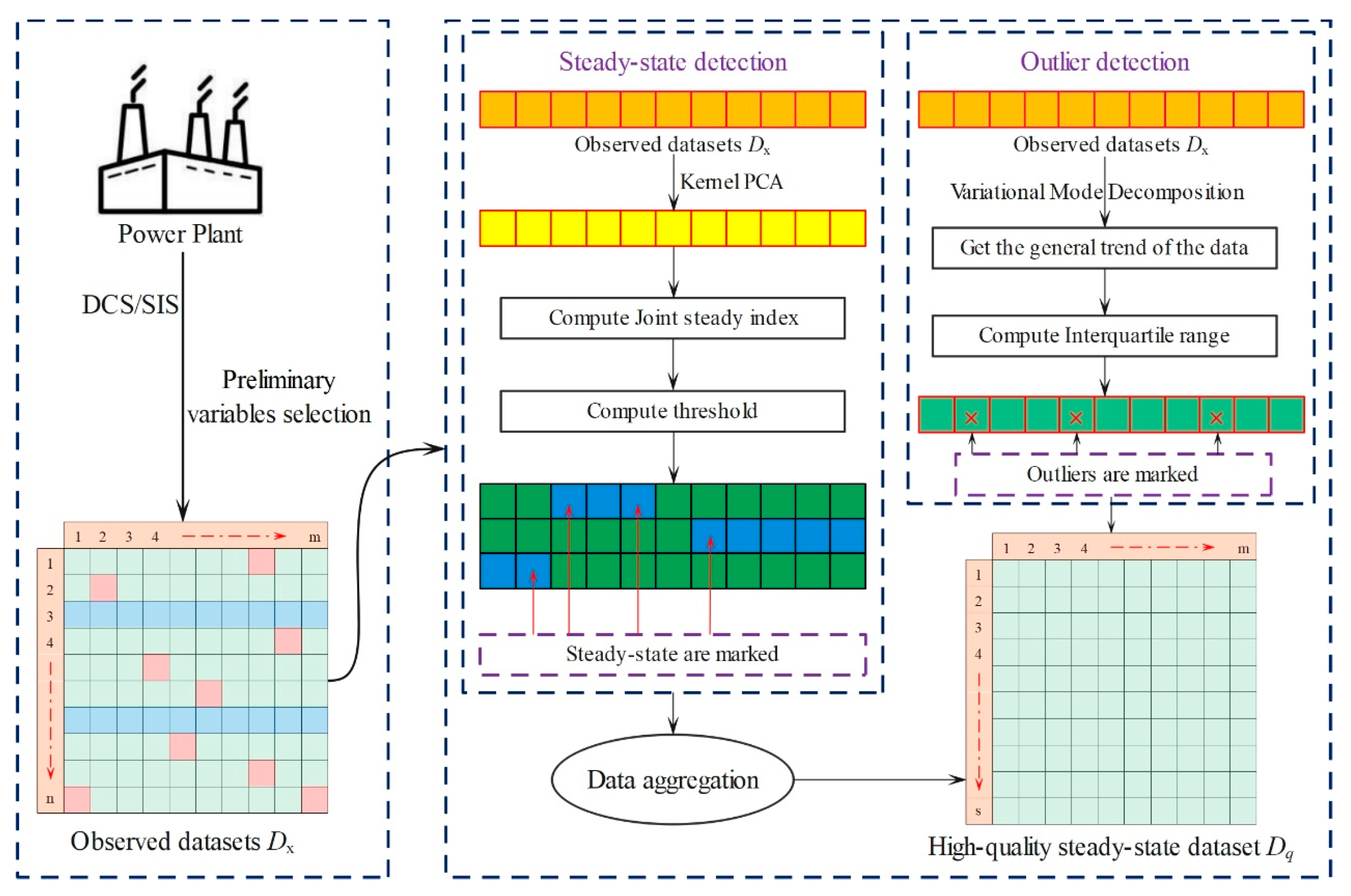
Due to the need to establish a case library that accurately reflects the mechanism relationship examined in this study, high-quality data corresponding to the steady-state operating conditions of the unit must be selected. Therefore, a robust filter framework is designed to filter out nonsteady-state and abnormal data. The data filtering process is shown in Figure 3.

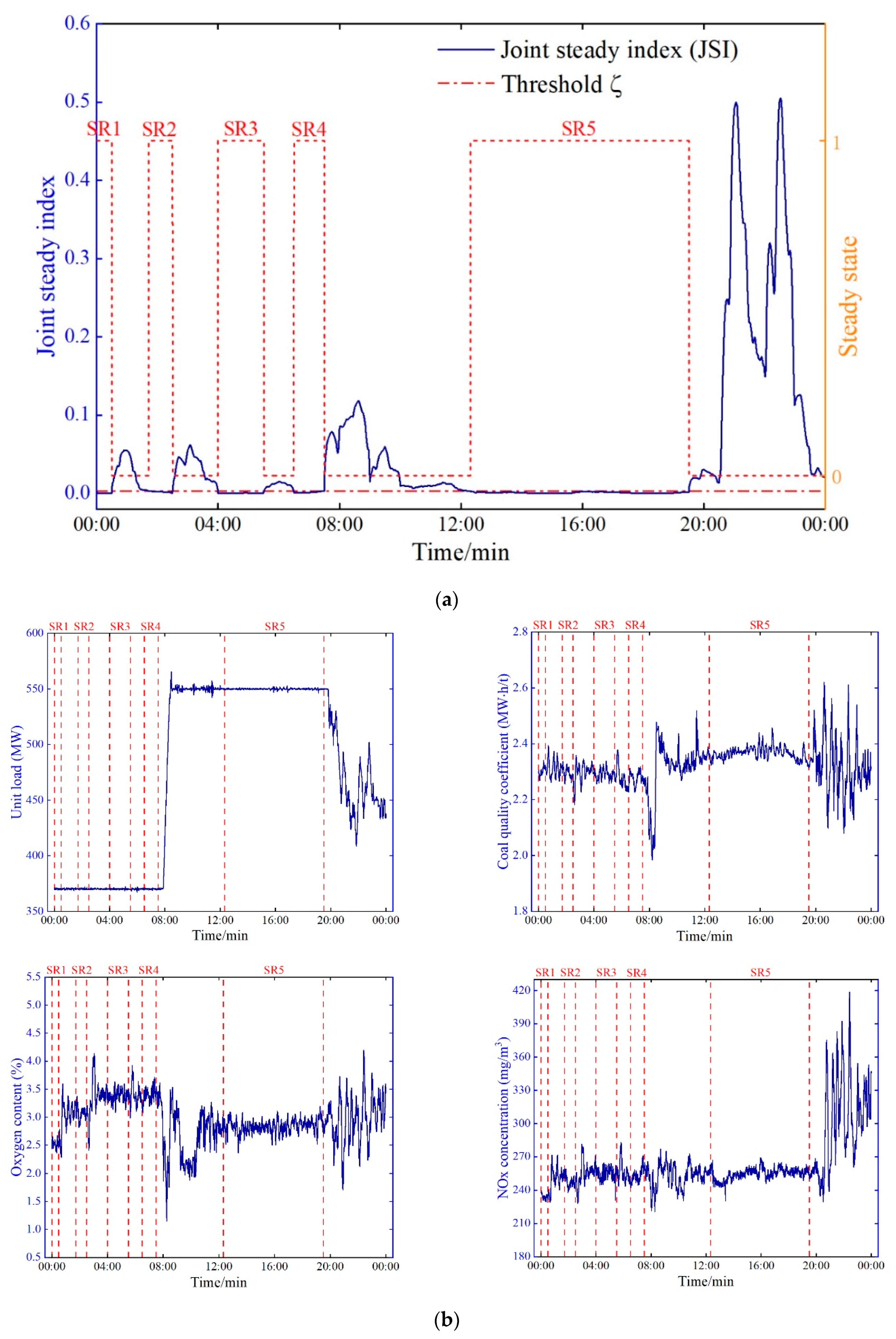
First, original data are collected from the plant’s supervisory information system (SIS) database. To obtain high-quality data samples that accurately reflect the static mechanism of the boiler combustion system, steady-state diagnosis and outlier detection are performed on the original observed data. Aiming at this process, a filter algorithm framework integrating steady-state diagnosis and outlier detection using a steady-state detection method based on kernel-PCA is proposed by comparing the joint steady index (JSI) with a given threshold and filtering the appropriate steady-state samples from the original observed data. In addition, the VMD algorithm is used to determine the data flow trend, and the outliers are determined by calculating the interquartile range to obtain the confidence interval. Finally, the data samples that passed the steady-state diagnosis and outlier detection are aggregated to form the high-quality steady-state dataset containing combustion system information.

3.1. Steady-State Identification

A sliding time window strategy is employed with the kernel-PCA algorithm for steady-state identification to determine the boiler’s operational status [24]. Given a matrix $X=[x_1,x_2,\cdots ,x_m{]}^{\mathrm{T}}$ with m variables and n observations and considering the need to eliminate the influence of dimensions, the matrix X is first normalized by the mean value to obtain a new matrix X’. For a specific variable x_i, the vector $d_{i,t}=[x_{i,t-T+1},\cdots ,x_{i,t}]$ represents the subset corresponding to a certain sliding time window T of the matrix X’. Therefore, the data under a sliding window can be expressed as $D_t=[d_{1,t},\cdots ,d_{m,t}]$, and the vector $d_{i,t}(i\in [1,m])$ can be mapped to the high-dimensional space by the kernel function $\varnothing$ to obtain $\chi =[{\varnothing }_1,{\varnothing }_2,\cdots ,{\varnothing }_m]$. Let S be the covariance matrix of the data samples in the feature space; then, the following formula is obtained:

$$(m-1)S={\chi }^T\chi ={\displaystyle \sum _{i=1}^m{\varnothing }_i{\varnothing }_i^T}$$

(2)

In this paper, the Gaussian kernel function is used:

$$K(d_i,d_j)=e^{-\gamma {‖d_i-d_j‖}^2}$$

(3)

where $K(\cdot ,\cdot )$ represents the kernel function and γ is a free parameter.

The calculation steps of the multivariate steady-state detection algorithm are as follows:

Step 1: Mean-normalize the original data to obtain a new matrix X′.

Step 2: Obtain the data D_t of the corresponding sliding time window, map it to the high-dimensional space through Equations (2) and (3), and obtain the result.

Step 3: Compute the covariance matrix S of $\chi$.

Step 4: Compute the l principal eigenvalues $\mathsf{\Lambda }={[{\lambda }_1,\cdots ,{\lambda }_l]}^T$ and eigenvectors $\mathsf{\Lambda }={[{\lambda }_1,\cdots ,{\lambda }_l]}^T$ of S, and arrange them in descending order.

Step 5: Compute the steady-state index vector $C=Q\mathsf{\Lambda }=[c_{t-T+1},\cdots ,c_t]$.

Step 6: Compute the joint steady index (JSI) according to the steady-state index vector C and Equation (4).

$$JSI=\sqrt{{\displaystyle \frac{1}{T-1}}{\displaystyle \sum _{k=t-T+1}^t{(c_k-\overline{c})}^2}}$$

(4)

Step 7: Compute the threshold $\zeta$ according to Equation (5).

$$\zeta =\lambda \sqrt{{\displaystyle \frac{1}{n}}{\displaystyle \sum _{i=1}^n{(JSI-\overline{JSI})}^2}}$$

(5)

where λ is a positive adjustment coefficient and $\overline{JSI}$ represents the average value of JSI.

Step 8: Judge whether $JSI<\zeta$ is true; if it is true, keep the data sample; otherwise, delete it.

3.2. Outlier Detection

Variational Modal Decomposition (VMD) is a signal decomposition algorithm [25] that divides the original signal into multiple signals from the perspective of the frequency domain and can be used to distinguish between normal and abnormal data [26]. To reasonably select the parameters of the VMD algorithm, the minimum envelope entropy [27] is used as the objective function, and the genetic algorithm is used to identify the best parameter combination for achieving the best signal decomposition effect and ensuring trend extraction accuracy. The envelope entropy is mathematically defined as follows:

$$E_p=-{\displaystyle \sum _{j=1}^m{p}_j\lg p_j}$$

(6)

$$p_j=a(j)/{\displaystyle \sum _{j=1}^{m}a(j)}$$

(7)

$$a(j)=\sqrt{{[x(j)]}^2+{\{H[x(j)]\}}^2}$$

(8)

where $a(j)$ represents the envelope signal sequence obtained after the signal $x(j)(j=1,2,\cdots ,m)$ is demodulated by Hilbert; H represents the Hilbert transform of the signal; and $p_j$ is the normalized form of $a(j)$.

The Pearson coefficient method is used to measure the degree of correlation between two variables; it is mathematically defined in Equation (9). In this paper, the effective signal is determined by judging the threshold in Equation (10), and the effective signal is reconstructed to extract the trend line. Herein, the decomposed signal with a Pearson coefficient greater than the threshold $\xi$ is effective.

$$C={\displaystyle \frac{Cov\left(x_i,y_i\right)}{{\sigma }_x{\sigma }_y}}$$

(9)

$$\xi ={\displaystyle \frac{C_{\max }}{10C_{\max }-3}}$$

(10)

where $Cov\left(x_i,y_i\right)$ and ${\sigma }_x,{\sigma }_y$ are the covariance and standard deviation of $x_i$ and $y_i$, respectively, and $C_{\max }$ is the maximum Pearson coefficient of each component and the original signal.

The trend extraction algorithm is shown in Figure 4. The specific process is as follows:

Step 1: Input the original signal f, set the range of K to [2, 9], and set the range of α to [1000, 3000].

Step 2: Use the GA to search [K, α]. VMD is input, the original signal is decomposed, and KIMF components are obtained.

Step 3: Calculate the minimum envelope entropy of the decomposed signal according to Equations (6)–(8).

Step 4: Choose the effective signal according to Equations (9) and (10).

Step 5: Repeat steps 2~4 to identify the minimum envelope entropy of the decomposed signal and its corresponding best parameters [K, α].

Step 6: Decompose the original signal with the best parameters [K, α] by VMD and choose the effective signal.

Step 7: Reconstruct the signal according to Equation (11) to obtain the best trend line.

$$f_{rec}={\displaystyle \sum _{i=1}^{N}IM{F}_i}$$

(11)

where $f_{rec}$ is the reconstruction signal and N is the number of effective signals.

For the data point $x(t)$ on the extracted trend curve, the confidence interval is calculated using the interquartile range method. For the original signal $f(t)$, if a data point is distributed outside the confidence interval, it is considered an outlier; otherwise, it is considered a normal point. The absolute error is first calculated according to Equation (12), and the confidence interval is calculated by Equation (13):

$$Error=\left|f(t)-x(t)\right|$$

(12)

$$\left\{\begin{array}{l}\hfill IQR=Q3-Q1\hfill \\ \hfill Bandwidth=Q3+1.5\times IQR\hfill \\ \hfill CI=[x(t)-B\mathrm{andwidth},x(t)+B\mathrm{andwidth}]\hfill \end{array}\right.$$

(13)

where Q1 and Q3 are the smaller and larger quartiles in the absolute error, respectively.

4. Offline and Online Optimization

4.1. Working Condition Case Library

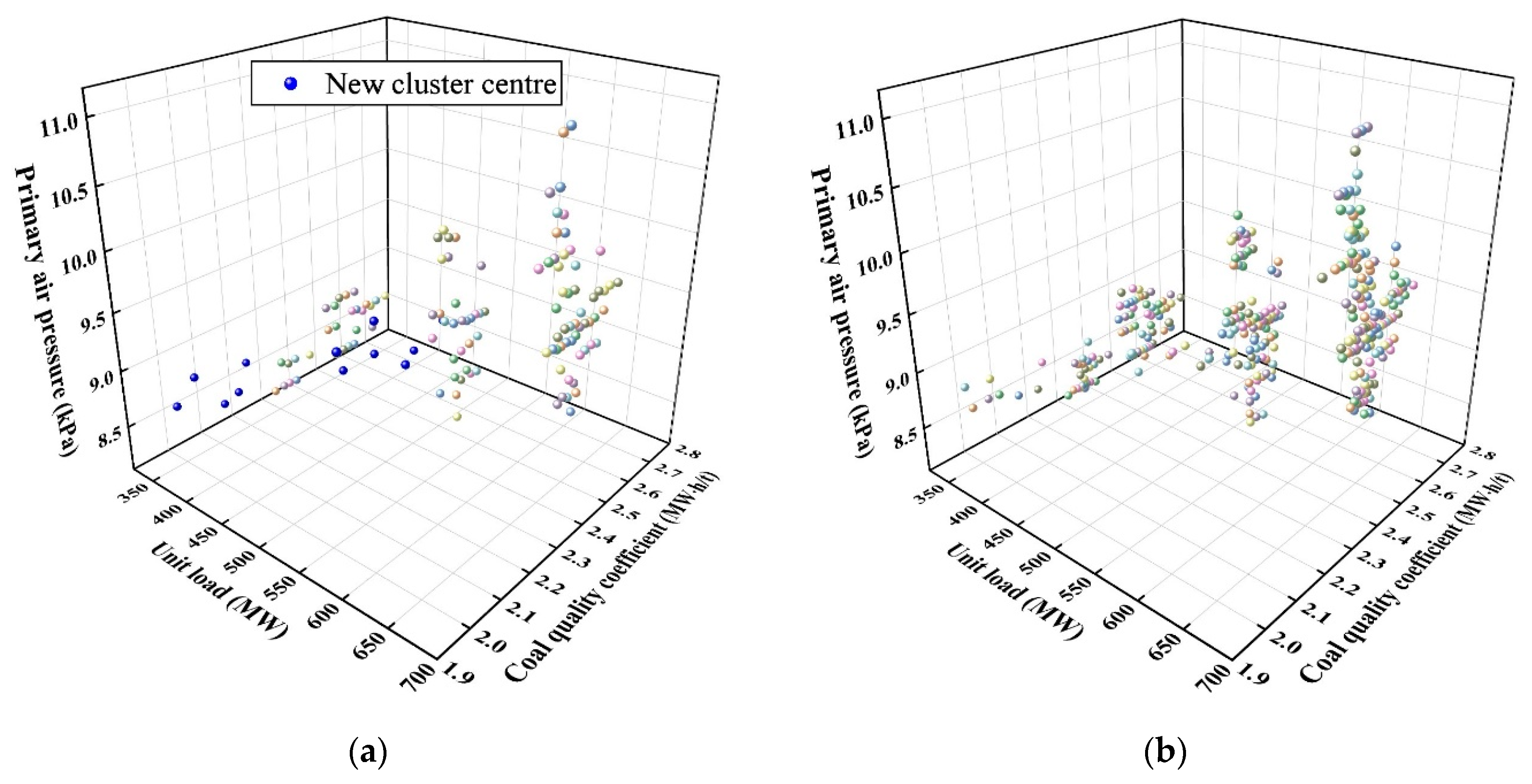
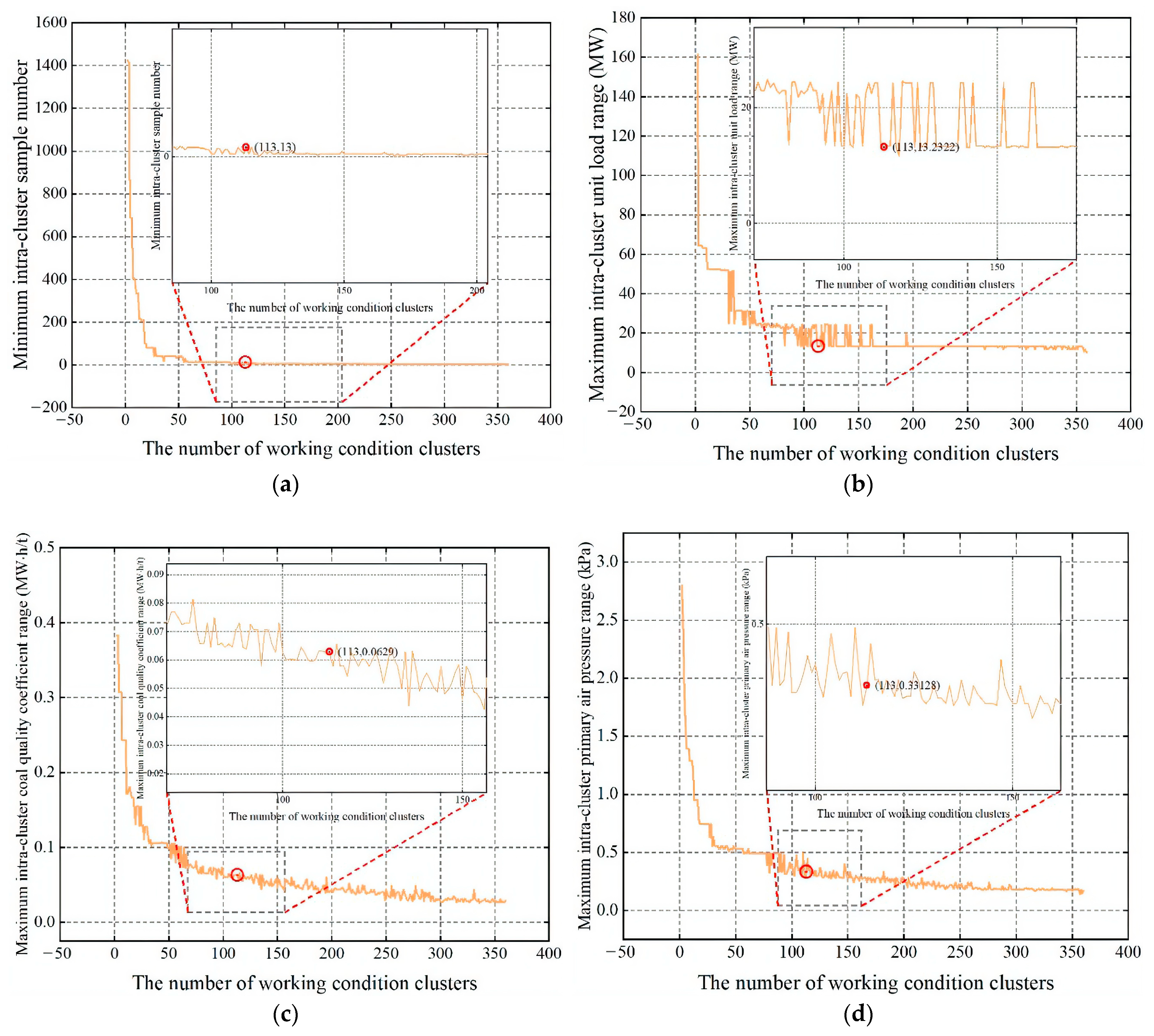
K-means++ [28] is used to cluster the three parameters that can reflect the operating state of the boiler, unit load, coal quality coefficient, and primary air pressure to construct an initial working condition case library. To consider the impact of data distribution changes on the case library, a reclustering strategy for the online adaptive calculation of working condition clusters is proposed.

According to engineering experience, when the working condition parameter range of data samples in a working condition cluster is kept within 2~3% of the parameter range in Table 1, the working condition division performs well. We thus use the maximum intracluster parameter range $\Delta x_i(i=1,2,3)$ determined in the previous round of working condition clustering as the judgment condition of the strategy to determine the number of clusters k in the new round of working conditions. The process of a new working condition clustering round is shown in Figure 5.

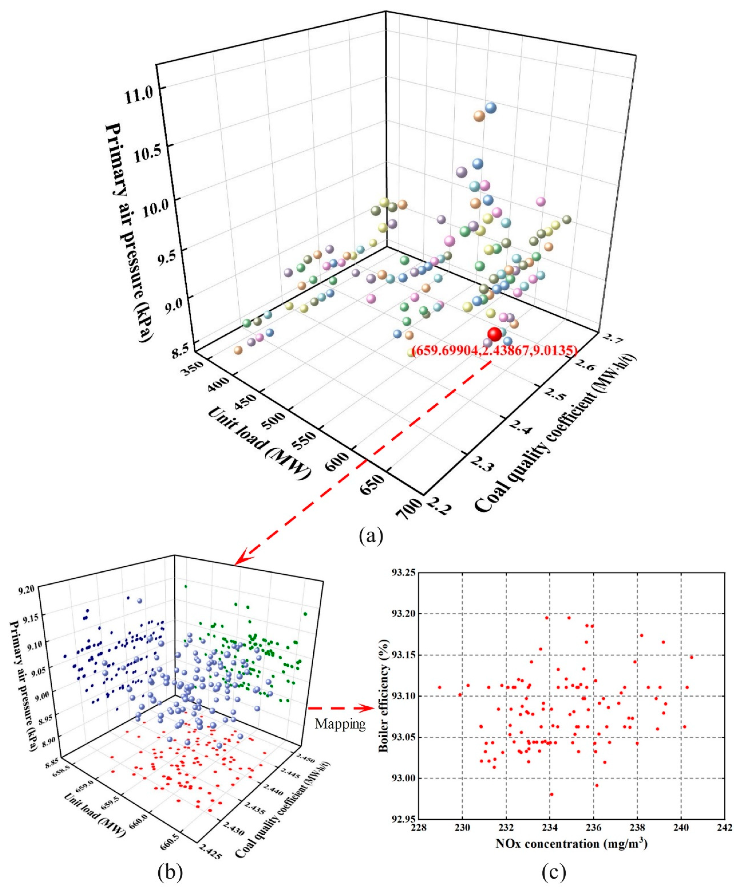
4.2. Preliminary Optimization

Based on the working condition case library, the initial boiler optimization case library is constructed by querying the two operating modes of the lowest NO_x concentration and the highest boiler efficiency for each working condition in the working condition case library. To find the case most similar to the target case, an online case retrieval strategy is presented for determining the optimization case.

First, the optimization case library is defined as O_n = (x_1,n, x_2,n, …, x_m,n, y_1,n, y_2,n), n = 1, 2, …, p, where p represents the total number of optimization cases; O_n represents the optimization case of the n-th working condition; $x_{m,n}$ represents the value of the m-th parameter of the n-th working condition optimization case; and $y_{1,n}$ and $y_{2,n}$ represent the boiler efficiency and NO_x concentration in the optimization case, respectively.

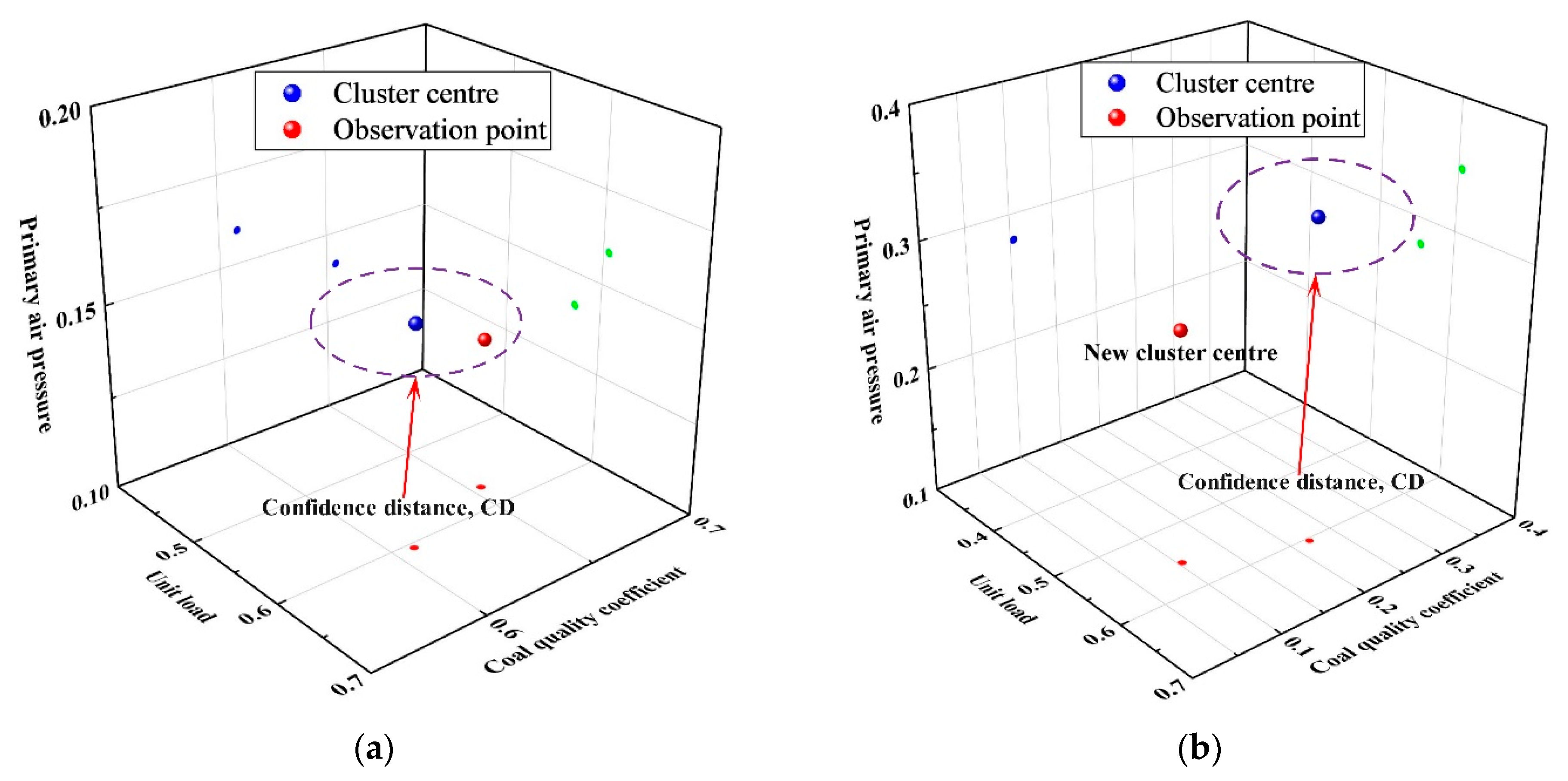
Second, the Euclidean distance between two points in space is the proximity, denoted as d, as shown in Equation (14). Then, the maximum proximity of all data samples of each operating condition in the operating condition case library to the center of that operating condition can be represented as $D_n=(d_1,d_2,\cdots ,d_n)$. Next, this section defines the confidence distance (CD) as $CD=\max (D_n)$.

$$Dis(x_i,x_j)=\sqrt{{\displaystyle \sum _{i=1}^m{(x_i-x_j)}^2}}$$

(14)

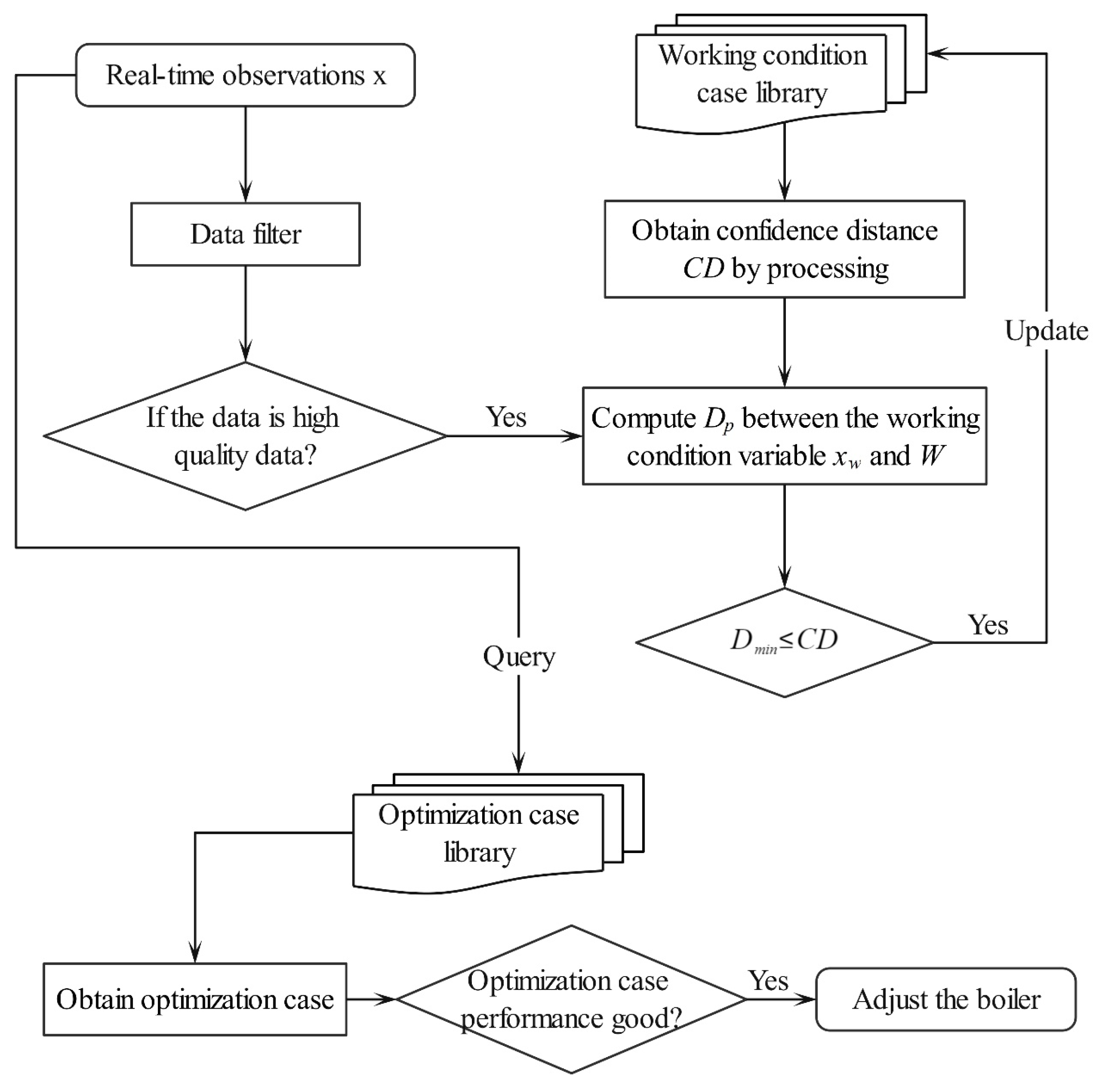
The online retrieval strategy based on the confidence distance is depicted in Figure 6. We provide the calculation steps of the store and update operation as follows:

Step 1: When observing a new data sample x, determine whether it passes the filter judgment; if it passes, the working condition variable of the data sample x is taken out as x_w; otherwise, the retrieval is stopped.

Step 2: The working condition variables and cluster centers in the working condition case library are normalized to obtain the normalized cluster center set $W=(w_1,w_2,\cdots ,w_n)$. CD is calculated from the normalized cluster center set.

Step 3: Normalize the current operating condition parameters $x_w$ to obtain $x_w^{\prime }$, and calculate their proximity with the normalized operating condition parameters in the library to obtain $D_p=(d_1,d_2,\cdots ,d_n)$.

Step 4: Calculate the minimum proximity $D_{\min }=\min (D_p)$ and judge whether $D_{\min }\le CD$ is true; if it is true, store it in the corresponding working condition case library.

4.3. Deep Optimization

Model-based optimization is conducted to improve the depth of the boiler optimization case library.

4.3.1. System Modeling

The boiler efficiency and NO_x emission model is constructed using XGBoost (Version 0.90). Its predicted value $\widehat{y_i}$ can be expressed as the sum of the results of multiple base models:

$$\widehat{y_i}={\displaystyle \sum _{k=1}^K{f}_k(x_i)},f_k\in N$$

(15)

where N is all the value spaces of the regression tree; K is the number of regression trees in the model; x_i is the input feature of the i-th sample; and $f_k(x_i)$ is the prediction result of the k-th tree. More details of the algorithm can be found in Ref. [29].

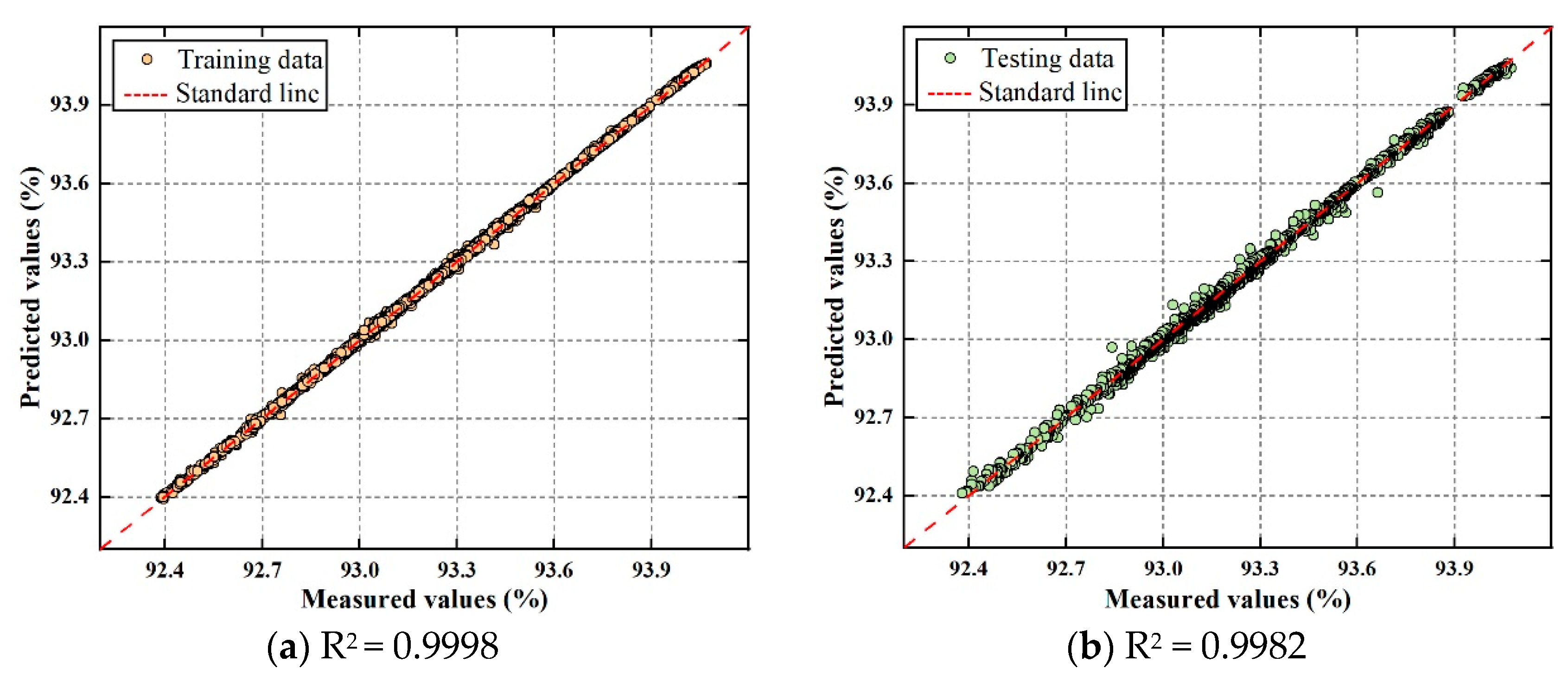
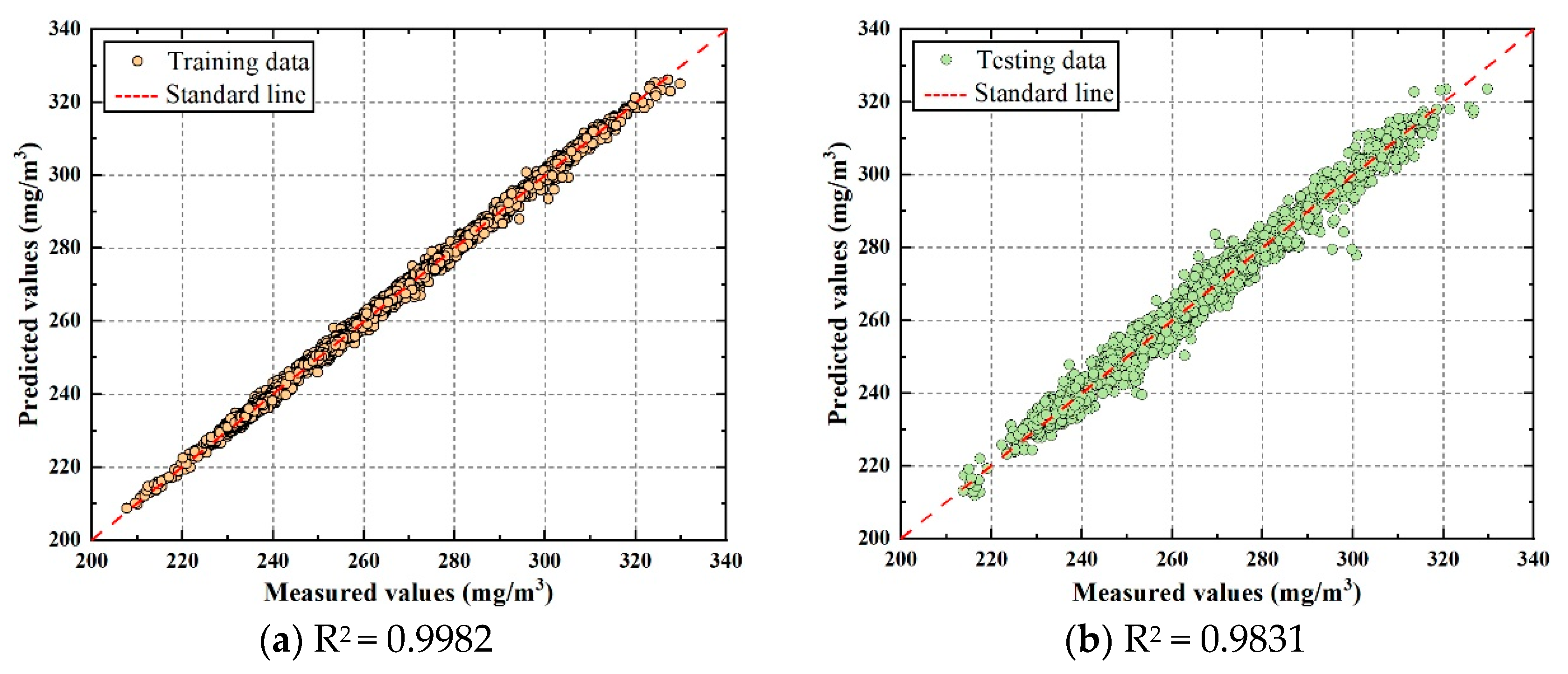
To evaluate performance, four evaluation metrics are used: mean absolute error (MAE), root mean square error (RMSE), mean absolute percentage error (MAPE), and R-squared (R²). Smaller MAE, RMSE, and MAPE values indicate a better predictive performance. The closer the R² value is to 1, the more accurate the model’s predictive performance is. The indices are calculated as follows:

$$\mathrm{MAE}={\displaystyle \frac{1}{n}}{\displaystyle \sum _{i=1}^n|{\widehat{y}}_i-y_i|}$$

(16)

$$\mathrm{RMSE}=\sqrt{{\displaystyle \frac{1}{n}}{\displaystyle \sum _{i=1}^n{\left({\widehat{y}}_i-y_i\right)}^2}}$$

(17)

$$\mathrm{MAPE}={\displaystyle \frac{1}{n}}{\displaystyle \sum _{i=1}^n\frac{|{\widehat{y}}_i-y_i|}{{\widehat{y}}_i}\times 100\%}$$

(18)

$$R^2=1-{\displaystyle \frac{{\Sigma }_{i=1}^n{\left(y_i-{\widehat{y}}_i\right)}^2}{{\Sigma }_{i=1}^n{\left(y_i-{\overline{y}}_i\right)}^2}}$$

(19)

where $y_i$, ${\widehat{y}}_i$, and ${\overline{y}}_i$ denote the measured value, predicted value, and average value of the prediction target, respectively.

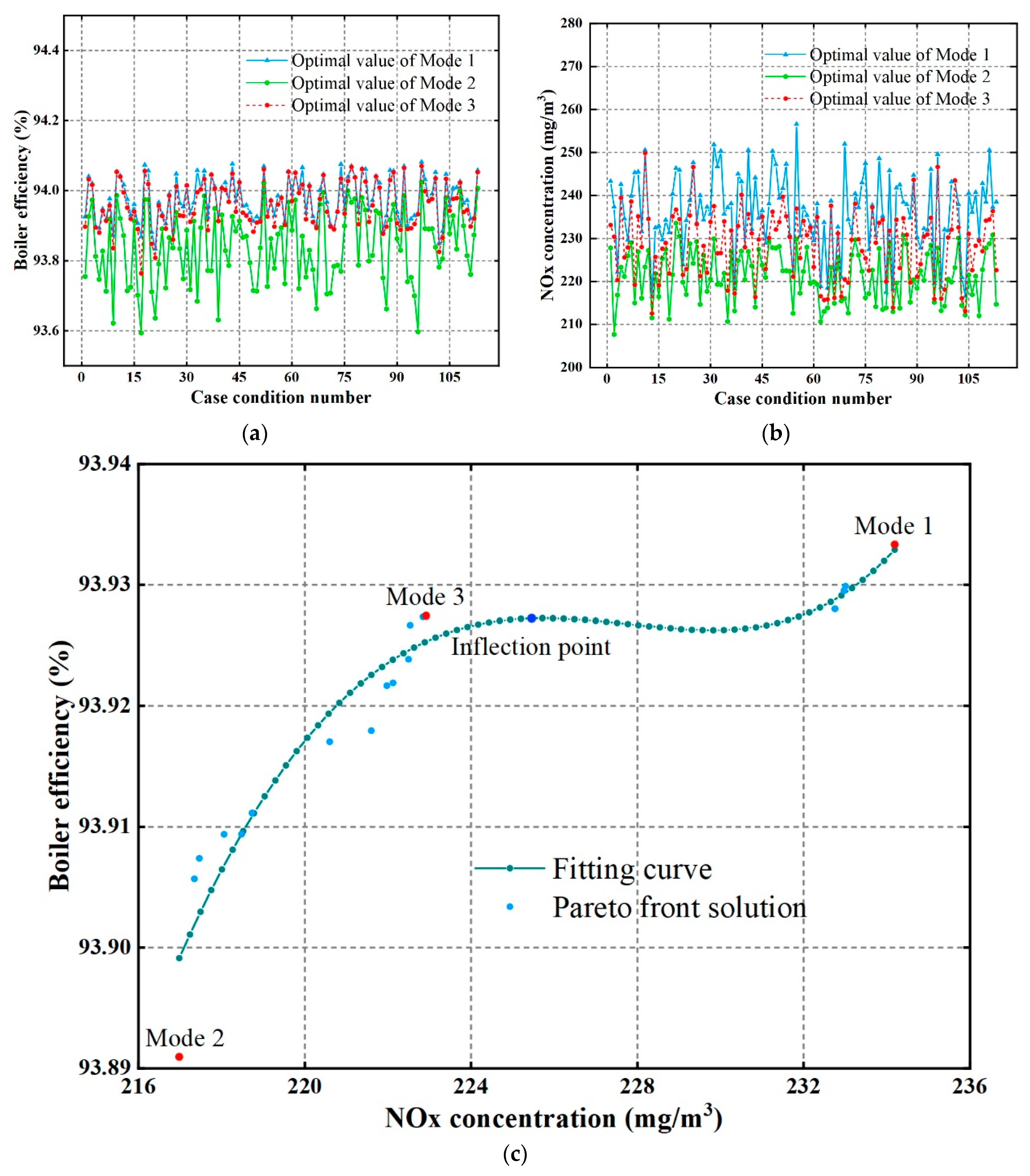
4.3.2. Multiobjective Optimization

NSGA-II [30] is used for combustion optimization, yielding a set of optimal optimization schemes, the Pareto front solution set. To quickly determine the only optimal optimization scheme in the equilibrium mode, an inflection point attribution strategy is proposed. The obtained Pareto solution set exhibits a distribution of an approximate concave function in the plane space, which has a maximum point, also known as an inflection point. In actual boiler combustion optimization, the inflection point indicates that when the boiler efficiency rises to a certain level, continuing to increase the small range efficiency will greatly increase the NO_x concentration in the boiler. Therefore, in the equilibrium mode, choosing the Pareto solution at the inflection point is the best optimization scheme. However, the distribution of the data samples of the Pareto solution set actually calculated by the NSGA-II algorithm is not uniform, making it difficult to identify the actual solution of the inflection point. To address this problem, a curve is first fit on the Pareto solution set space using polynomial fitting, and the curve is then discretized with a certain sampling interval to calculate the inflection point X_m on the fitted curve, and the closest Pareto solution to X_m is identified as the best optimization solution in the equilibrium mode.

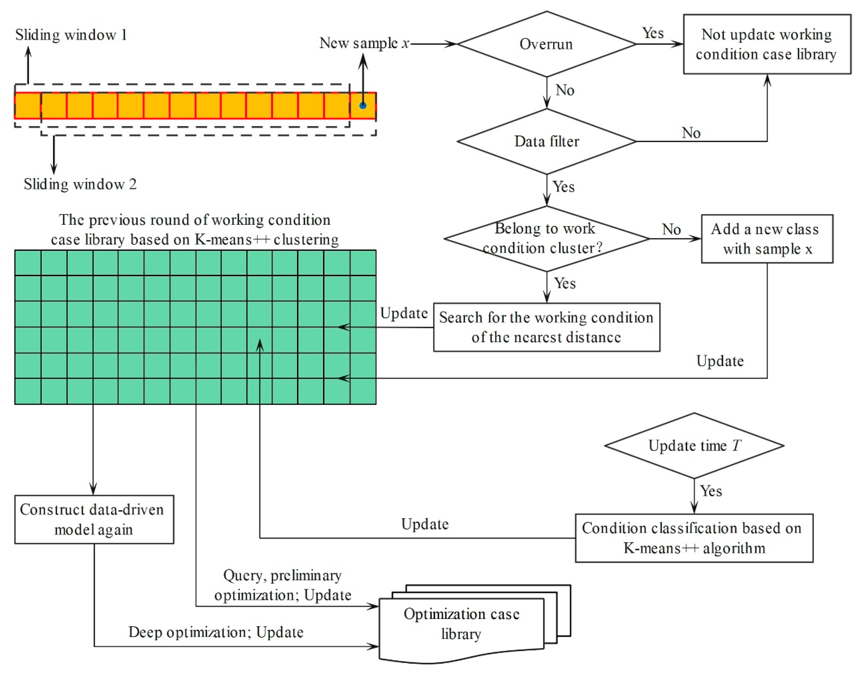
4.4. Adaptive Update Strategy

To consider the variation in the working condition case library over time, an online adaptive update strategy is proposed. The strategy is shown in Figure 7, and the steps are as follows:

Step 1: The data filter is used to extract high-quality data samples D_q from the original data, and then the K-means++ algorithm is used to divide the working conditions and construct the initial boiler working condition case library; the online adaptive update period is defined as T.

Step 2: When a new data sample x is observed in real time, whether it is overrun is evaluated; if it is, the working condition case library is not updated.

Step 3: The data filter is used to determine whether x is a high-quality data sample; if it is, Step 4 is carried out; otherwise, the working condition case library is not updated.

Step 4: Using the online retrieval strategy, whether x belongs to the existing working condition cluster is judged; if it is, x will be stored in the nearest working condition cluster; otherwise, a new category of working conditions is added with the data sample as the cluster center and updated synchronously in the optimization case library.

Step 5: Steps 2~4 are repeated until the adaptive update period T is reached; at this time, the working conditions are reclassified based on the K-means++ algorithm to construct the working condition case library and the optimization case library. The data-driven model is trained based on the reconstructed working condition case library. After training, the model is updated online, and the optimization case library is updated again.

Step 6: The timing is repeated until the adaptive update period T is reached, and a new round of data and model updates is conducted.

5. Results and Discussion

5.1. Data Filtering Results

Figure 8 shows the steady-state detection results of the 24 h sampling points of the utility boiler. The boiler has a total of five steady-state ranges (SRs) in the 24 h. The results show that the proposed filter successfully retains the steady-state samples, performing well.

Figure 9 shows the outlier detection results for the sampling points of the utility boiler on the same day, where original data are represented by black dots, trends are represented by dashed yellow lines, confidence intervals are represented by blue areas, and outliers are represented by red hollow circles. The results indicate that the designed filter has good outlier detection ability. The filter is conducted for 72,000 observation data points of utility boilers over 25 days. After the above filtering operations, 6392 high-quality steady-state operating data are maintained as the initial samples for constructing the working condition case library, data-driven model, and optimization case library.

5.2. Construction of the Working Condition Case Library

Clustering and corresponding analysis are performed on the obtained 6392 high-quality data samples. First, the range of the hyperparameter k for the K-means++ algorithm is set to [2, 360], and the minimum intracluster sample number and the maximum intracluster working condition parameter range are calculated. Then, k = 113 is determined to be the number of working condition clusters for the initial clustering. Finally, Figure 10 illustrates that when k = 113, there are at least 13 high-quality data samples in each working cluster in the working condition case library to reflect the mechanism relationship under this working condition. In each working cluster, the range of working condition parameters can be kept below 3% of the overall variation range, which is sufficient for showing that this method has a good working condition division effect.

According to the above analysis, 6392 high-quality data samples are preliminarily divided into 113 working conditions. In Figure 11, (a) shows the spatial distribution of the centers of all condition clusters, with each sphere representing a class of boiler operating conditions, (b) represents the distribution of condition cluster samples for the working condition [659.7 MW, 2.44 MW·h/t, 9.01 kPa], and (c) represents the projection of the data samples in (b) onto the NO_x concentration and boiler efficiency dimensions.

This figure illustrates that the distribution of a single working condition cluster in the sample space is relatively uniform, and the projection figure illustrates that although the optimization method based on the case library for directly adjusting the boiler is real, simple, and fast, the case library samples often do not present an equilibrium solution like the Pareto front. Therefore, deep optimization is essential for the online boiler optimization.

5.3. Construction of the Data-Driven Model

5.3.1. Model Training

From the 6392 data samples of the above 113 types of working conditions, 70% of the data samples of each working condition are selected to form the model training set, and the remaining 30% of the data are used as the testing set for evaluating the model performance. After the dataset is reconstructed, the operating condition parameters and performance parameter ranges of the training set and testing set are shown in

Table 4. Dataset reconstruction results.

Description	Training Set	Testing Set
Unit load	[368.64, 668.61]	[368.46, 662.07]
Coal quality coefficient	[2.22, 2.65]	[2.23, 2.64]
Primary air pressure	[8.37, 11.20]	[8.31, 11.10]
Boiler efficiency	[92.39, 94.07]	[92.38, 94.07]
NOx concentration	[207.69, 329.90]	[213.84, 329.83]
Count	4426	1966

.

First, the parameters n_estimators, subsample, and colsample_bytree of the XGBoost model are preliminarily determined to be 365, 0.3, and 0.7, respectively. In addition, the model is trained using a GA and a five-fold cross-validation method to determine the model hyperparameters. The optimal hyperparameters of the boiler efficiency model and the NO_x emission model are provided in

Table 5. Result of hyperparameter optimization of the XGBoost model.

Description	Range	Boiler Efficiency Model	NOx Emission Model
Learning_rate	[1 × 10−8, 0.1]	0.0810	0.0319
Max_depth	[3, 25]	19	24
Min_child_weight	[1, 10]	7.0224	1
gamma	[1 × 10−8, 10]	1 × 10−8	1.8735

.

5.3.2. Model Evaluation

Figure 12 and Figure 13 show the predictive performance of the boiler efficiency model and NO_x emission model on the training and testing datasets, respectively. The training data (R² = 0.9998) and testing data (R² = 0.9982) of the boiler efficiency model and the training data (R² = 0.9982) and testing data (R² = 0.9831) of the NO_x emission model are obviously distributed near the standard line. The results show that the characteristic model of the boiler combustion system has good predictive performance.

The specific prediction performances of the two combustion characteristic models are provided in

Table 6. Result of model evaluation.

	Boiler Efficiency Model		NOx Emission Model
	Training Set	Testing Set	Training Set	Testing Set
MAE	0.0031	0.0104	0.7677	2.3672
RMSE	0.0049	0.0154	1.0225	3.1429
MAPE (%)	0.0034	0.0111	0.2923	0.8997
R2	0.9998	0.9982	0.9982	0.9831

.

5.4. Construction of the Optimization Case Library

The multiobjective combustion optimization problem is described as Equation (20).

$$\left\{\begin{array}{c}Const=f_w(x_1,x_2,x_3)\\ \max \eta =f_{\eta }(f_w(x_1,x_2,x_3),x_4,x_5,\cdots ,x_{30})\hfill \\ \min N{O}_x=f_{N{O}_x}(f_w(x_1,x_2,x_3),x_4,x_5,\cdots ,x_{30})\hfill \\ \hfill s.t.x_{i\min }\le x_i\le x_{i\max }\hfill \\ \hfill 4\le i\le 30\hfill \end{array}\right.$$

(20)

where Const represents three working condition parameters; f_w represents the K-means++ algorithm or the online retrieval strategy; x₄~x₃₀ are the operable parameters in Table 2, which are also the parameters for the multiobjective optimization solution in this paper; and f_η and f_NOx represent data-driven models for boiler efficiency and NO_x concentration, respectively. In the multiobjective optimization calculation, the upper limit and lower limit of oxygen content are set as 1.5% and 6%, respectively; the optimization range of damper opening is set as [0%, 100%].

Combustion optimization is conducted for different goals: (1) Mode 1: the boiler combustion efficiency is optimal; (2) Mode 2: the NO_x emission concentration is optimal; (3) Mode 3: the boiler combustion efficiency and NO_x emission concentration are balanced. Figure 14 and Figure 15 show the comparison results of Mode 1 and Mode 2 using the query optimization strategy, intelligent optimization strategy, and hybrid optimization strategy proposed in this paper, respectively. Compared with the original operation condition, the three strategies all exhibit more effective optimization, especially the optimization method proposed in this paper, which performs well under all working conditions. Meanwhile, since the best optimization cases for Mode 1 and Mode 2 are primarily drawn from the Pareto front solution set, many operational conditions’ best optimization cases achieve high efficiency or low pollution compared to the original cases while ensuring their optimal objectives. Notably, a very small number of operational conditions’ best optimization cases are derived from historical observation data.

Figure 16a,b display the optimal solutions for all operational conditions in Modes 1 to 3, successfully demonstrating that Mode 3 is the most suitable combustion mode for achieving high efficiency and low pollution. Figure 16c illustrates the effectiveness of the inflection point attribution strategy through a working condition example, providing an adaptive computational approach for solving Mode 3 for online combustion optimization. Based on the above calculations and strategies, the best optimization schemes of Modes 1~3 are selected for all working conditions, and an initial optimization case library is constructed, providing a basic guarantee for boiler parameter adjustments.

5.5. Effective Analysis of the Proposed Strategy

5.5.1. Analysis of the Online Retrieval Strategy

In this section, we analyze the impact of the online retrieval process on the case library. Figure 17 shows the changes in the cluster center and data distribution in the normalized space with the working condition case library when a new set of high-quality data samples is observed by the system. As shown in Figure 17a, when the Euclidean distance between a new sample and the nearest cluster center is less than the CD, the new sample belongs to the working condition and is stored in the case library. As shown in Figure 17b, when the Euclidean distance between a new sample and the nearest cluster center is greater than the CD, there is no matching working condition in the case library. In this case, a new working condition is created in the case library with the new sample as the cluster center, and this condition is populated with the optimal solutions for the three optimization modes based on this sample. Before the update period T is reached, the case base is updated using this method during the real-time retrieval process of the case base. Figure 18a shows the change in distribution in the cluster center before adaptive updating.

5.5.2. Analysis of the Reclustering Strategy

In this section, we verify the effectiveness of the proposed reclustering strategy. Figure 18a,b show the changes in the cluster center in the case library before and after the adaptive reclustering strategy, respectively. Due to the increasing richness of data samples in the case library during the online retrieval process, after reclustering, the data samples are divided into 313 working conditions. The maximum intracluster unit load range, the maximum intracluster coal quality coefficient range, and the maximum intracluster primary air pressure range are 13.2 MW, 0.049 MW∙h/t, and 0.206 kPa, respectively. The results show that the proposed reclustering strategy can satisfy the online adaptive computation and the range of 2~3% working condition parameters.

5.6. Online Combustion Optimization Experiment

In this section, we conduct online testing using future data for the same utility boiler, including multiple steady-state and transient processes. In the experiment, when a new data point is observed, the system immediately extracts its condition parameters $[x_1,x_2,x_3]$ and uses the online retrieval strategy to query optimization solutions from the case library and adjust the boiler operating parameters accordingly. The software and hardware configurations used in this study are detailed in

Table 7. Software and hardware configurations.

Description	Configuration
OS	Windows 11 × 64
CPU	Intel(R) Core(TM) i7-9750H CPU @2.60 GHz 2.59 GHz
Memory	16 GB DDR4 3200 MHz
Python version	3.7.12

.

Figure 19a,b show the optimization results of Mode 1 and Mode 2, respectively; Figure 20 shows the optimization results of Mode 3. After testing, the results show that the operation optimization of the unit using the traditional data-driven model and intelligent optimization algorithm takes approximately 3 to 5 min, which obviously does not meet the real-time requirements of online combustion optimization. Since the proposed optimization method can basically obtain the optimal solution within 1 s (0.95~6.99 ms), it has an important calculation speed advantage in online combustion optimization. Finally, as shown in Figure 19 and Figure 20, the proposed optimization method can improve boiler efficiency, reduce NO_x concentration, and effectively achieve the online boiler combustion optimization task.

6. Conclusions

To address the time-consuming limitation of traditional combustion optimization methods, this study proposes a novel online combustion optimization framework integrating data filtering, case-based reasoning, data-driven modeling, and multiobjective optimization. The proposed method has been validated on a 660 MW utility boiler, demonstrating its ability to enhance combustion performance while ensuring a swift response to changing operating conditions. The key conclusions of this study are as follows:

(1)

The robust data filter using Kernel-PCA, JSI, and VMD extracts 6392 high-quality steady-state samples from 72,000 original data points. The filter successfully retains steady-state data, removes anomalies, and identifies five steady-state periods within a 24 h dataset, demonstrating its efficiency in data pre-processing for combustion optimization.

(2)

Based on the extracted samples, combustion system models were developed using XGBoost. The boiler efficiency model achieved R² values of 0.9998 and 0.9982 for the training and test sets, respectively, while the NOx emissions model attained R² values of 0.9982 and 0.9831, effectively capturing the relationships between operational parameters and combustion performance.

(3)

K-means clustering was used to construct the working condition case library, while NSGA-II, combined with combustion system models and inflection point attribution strategy, optimized each condition to develop an optimization case library. This approach lowered NOx emissions from 329.90 mg/m³ to 213.84 mg/m³, a 35.2% reduction, while increasing boiler efficiency from 92.39% to 94.07%, enhancing both environmental and operational performance.

(4)

In terms of speed, an online retrieval strategy based on CD quickly identifies the optimal case for real-time operation, enabling optimization in just 0.95–6.99 milliseconds, outperforming traditional methods requiring 3–5 min. A reclustering strategy dynamically updates the case library, expanding the number of working conditions from 113 to 313, ensuring that the optimization method remains effective under varying operating conditions.

Future research will focus on developing a dynamic combustion optimization approach based on a dynamic working condition case library. The proposed research direction involves employing deep learning techniques to extract latent features from time-series data of non-adjustable variables, serving as the basis for dynamic case library segmentation, aiming to further enhance the adaptability and effectiveness of intelligent combustion optimization.

References

1. Wang, Y.N.; Zhao, C.H. A deep graph convolutional network model of NOx emission prediction for coal-fired boiler. Can. J. Chem. Eng. 2024, 102, 669–684. [Google Scholar] [CrossRef]
2. Baqain, M.; Neshumayev, D.; Konist, A. NOx and N2O emissions from Ca-rich fuel conversion in oxyfuel circulating fluidized bed combustion. Therm. Sci. Eng. Prog. 2023, 42, 101938. [Google Scholar] [CrossRef]
3. Khanali, M.; Akram, A.; Behzadi, J.; Rad, F.M.; Saber, Z.; Chau, K.W.; Pelesaraei, A.N. Multi-objective optimization of energy use and environmental emissions for walnut production using imperialist competitive algorithm. Appl. Energy 2021, 284, 116342. [Google Scholar] [CrossRef]
4. Liu, Y.; Zhou, J.X.; Fan, W. A novel robust dynamic method for NOx emissions prediction in a thermal power plant. Can. J. Chem. Eng. 2023, 101, 2391–2402. [Google Scholar] [CrossRef]
5. Chen, S.; Yu, C.; Zhu, Y.K.; Fan, W.; Yu, H.Q.; Zhang, T.H. NOx formation model for utility boilers using robust two-step steady-state detection and multimodal residual convolutional auto-encoder. J. Taiwan Inst. Chem. Eng. 2024, 155, 105252. [Google Scholar] [CrossRef]
6. Zhu, Y.K.; Yu, C.; Jin, W.; Shi, L.; Chen, B.; Xu, P. Mechanism-enhanced data-driven method for the joint optimization of boiler combustion and selective catalytic reduction systems considering gas temperature deviations. Energy 2024, 291, 130432. [Google Scholar] [CrossRef]
7. Chang, J.; Wang, W.; Zhou, Z.J.; Chen, H.G.; Niu, Y.G. CFD modeling of hydrodynamics, combustion and NOx emission in a tangentially fired pulverized-coal boiler at low load operating conditions. Adv. Powder Technol. 2021, 32, 290–303. [Google Scholar] [CrossRef]
8. Sun, D.P.; Fang, Q.Y.; Wang, H.J.; Zhou, H.C. A compact optimization strategy for combustion in a 125 MW tangentially anthracite-fired boiler by an artificial neural network. Asia-Pac. J. Chem. Eng. 2008, 3, 432–439. [Google Scholar] [CrossRef]
9. Aliramezani, M.; Koch, C.R.; Shahbakhti, M. Modeling, diagnostics, optimization, and control of internal combustion engines via modern machine learning techniques: A review and future directions. Prog. Energy Combust. Sci. 2002, 88, 100967. [Google Scholar] [CrossRef]
10. Yang, T.T.; Liu, J.Z.; Zeng, D.L.; Xie, X. Application of data mining in boiler combustion optimization. In Proceedings of the 2010 the 2nd International Conference on Computer and Automation Engineering (ICCAE), Singapore, 26–28 February 2010; Volume 2, pp. 225–228. [Google Scholar]
11. Zhao, W.J.; Liu, C. The optimizing for boiler combustion based on fuzzy association rules. In Proceedings of the 2011 International Conference of Soft Computing and Pattern Recognition (SoCPaR), Dalian, China, 14–16 October 2011; pp. 306–311. [Google Scholar]
12. Kusiak, A.; Song, Z. Combustion efficiency optimization and virtual testing: A data-mining approach. IEEE Trans. Ind. Inform. 2006, 2, 176–184. [Google Scholar] [CrossRef]
13. Kusiak, A.; Song, Z. Clustering-Based Performance Optimization of the Boiler-Turbine System. IEEE Trans. Energy Convers. 2008, 23, 651–658. [Google Scholar] [CrossRef]
14. Kusiak, A.; Song, Z. Constraint-Based Control of Boiler Efficiency: A Data-Mining Approach. IEEE Trans. Ind. Inform. 2007, 3, 73–83. [Google Scholar]
15. Zhou, H.; Cen, K.F.; Fan, J.R. Multi-objective optimization of the coal combustion performance with artificial neural networks and genetic algorithms. Int. J. Energy Res. 2005, 29, 499–510. [Google Scholar] [CrossRef]
16. Wang, C.L.; Liu, Y.; Zheng, S.; Jiang, A.P. Optimizing combustion of coal fired boilers for reducing NOx emission using Gaussian Process. Energy 2018, 153, 149–158. [Google Scholar] [CrossRef]
17. Song, J.G.; Romero, C.E.; Yao, Z.; He, B.S. Improved artificial bee colony-based optimization of boiler combustion considering NOx emissions, heat rate and fly ash recycling for on-line applications. Fuel 2016, 172, 20–28. [Google Scholar] [CrossRef]
18. Ma, Y.P.; Wang, H.Q.; Zhang, X.X.; Hou, L.K.; Song, J.C. Three-objective optimization of boiler combustion process based on multi-objective teaching–learning based optimization algorithm and ameliorated extreme learning machine. Mach. Learn. Appl. 2021, 5, 100082. [Google Scholar] [CrossRef]
19. Rahat, A.A.M.; Wang, C.L.; Everson, R.M.; Fieldsend, J.E. Data-driven multi-objective optimisation of coal-fired boiler combustion systems. Appl. Energy 2018, 229, 446–458. [Google Scholar] [CrossRef]
20. Feng, K.; He, D.F.; Xu, A.J.; Wang, H.B. End Temperature Prediction of Molten Steel in RH Based on Case-based Reasoning with Optimized Case Base. J. Iron Steel Res. Int. 2015, 22, 68–74. [Google Scholar] [CrossRef]
21. Xia, J.; Chen, G.; Tan, P.; Zhang, C. An online case-based reasoning system for coal blends combustion optimization of thermal power plant. Int. J. Electr. Power Energy Syst. 2014, 62, 299–311. [Google Scholar] [CrossRef]
22. Zheng, W.; Wang, C.; Yang, Y.J.; Zhang, Y.F. Multi-objective combustion optimization based on data-driven hybrid strategy. Energy 2020, 191, 116478. [Google Scholar] [CrossRef]
23. Yu, C.; Xiong, W.; Ma, H.; Zhou, J.X.; Si, F.Q.; Jiang, X.M.; Fang, X.W. Numerical investigation of combustion optimization in a tangential firing boiler considering steam tube overheating. Appl. Therm. Eng. 2019, 154, 87–101. [Google Scholar] [CrossRef]
24. Fan, W.; Si, F.Q.; Ren, S.J.; Yu, C.; Cui, Y.F.; Wang, P. Integration of continuous restricted Boltzmann machine and SVR in NOx emissions prediction of a tangential firing boiler. Chemom. Intell. Lab. Syst. 2019, 195, 103870. [Google Scholar] [CrossRef]
25. Dragomiretskiy, K.; Zosso, D. Variational mode decomposition. IEEE Trans. Signal Process. 2014, 62, 531–544. [Google Scholar] [CrossRef]
26. Zhu, Y.K.; Yu, C.; Fan, W.; Yu, H.Q.; Jin, W.; Chen, S.; Liu, X. A novel NOx emission prediction model for multimodal operational utility boilers considering local features and prior knowledge. Energy 2023, 280, 128128. [Google Scholar] [CrossRef]
27. Fischer, J.; Doolan, C. An improved eigenvalue background noise reduction method for acoustic beamforming. Mech. Syst. Signal Process. 2020, 140, 106702. [Google Scholar] [CrossRef]
28. Arthur, D.; Vassilvitskii, S. K-means++ the advantages of careful seeding. In Proceedings of the Eighteenth Annual ACM-SIAM Symposium on Discrete Algorithms, New Orleans, Louisiana, 7–9 January 2007; pp. 1027–1035. [Google Scholar]
29. Chen, T.Q.; Guestrin, C. Xgboost: A scalable tree boosting system. In Proceedings of the 22nd ACM SIGKDD International Conference on Knowledge Discovery and Data Mining, San Francisco, CA, USA, 13–17 August 2016; pp. 785–794. [Google Scholar]
30. Deb, K.; Pratap, A.; Agarwal, S.; Meyarivan, T. A fast and elitist multiobjective genetic algorithm: NSGA-II. IEEE Trans. Evol. Comput. 2002, 6, 182–197. [Google Scholar] [CrossRef]
Figure 1. Schematic diagram of the supercritical coal-fired boiler.
Processes 13 00469 g001
Figure 2. Structural diagram of the boiler online combustion optimization method. The red arrow in the figure indicates the application of optimization case library for online optimization.
Processes 13 00469 g002
Figure 3. Flow chart of the filter designed in this paper. The blue square represents unsteady-state data. The green square represents steady-state data. The red cross represents outlier data.
Processes 13 00469 g003
Figure 4. Flow chart of trend extraction based on GA-VMD.
Processes 13 00469 g004
Figure 5. Flow chart of the reclustering strategy.
Processes 13 00469 g005
Figure 6. Flow chart of the online retrieval strategy.
Processes 13 00469 g006
Figure 7. Flow chart of the adaptive update strategy. The orange square represents the operating data and the green square represents the working condition case library.
Processes 13 00469 g007
Figure 8. An example of steady-state identification in a typical 24 h. (a) Joint steady index, threshold, and original data. (b) Steady-state identification results for four variables.
Processes 13 00469 g008
Figure 9. An example of outlier detection in a typical 24 h. The red circle represents the outliers, the blue represents the confidence interval, and the yellow represents the trend line of the data stream.
Processes 13 00469 g009
Figure 10. Statistical charts for choosing k. (a) The minimum intracluster sample number changes with the number of clusters. (b) The maximum intracluster unit load range changes with the number of clusters. (c) The maximum intracluster coal quality coefficient range changes with the number of clusters. (d) The maximum intracluster primary air pressure range changes with the number of clusters.
Processes 13 00469 g010
Figure 11. Case clustering and projection plots. (a) The distribution of cases in the case library. Dots of different colors represent the cases at different regions. (b) The distribution of data points in a certain case. The blue dots represent the projections of the data points on the plane of primary air pressure and coal quality coefficient. The red dots represent the projections of the data points on the plane of unit load and coal quality coefficient. The green dots represent the projections of the data points on the plane of unit load and primary air pressure. (c) The projections of the data points on the performance index plane (i.e., boiler efficiency and NOx concentration).
Processes 13 00469 g011
Figure 12. Comparison of the actual measured and predicted boiler efficiency values: (a) training dataset and (b) testing dataset.
Processes 13 00469 g012
Figure 13. Comparison of the actual measured and predicted NOx values: (a) training dataset and (b) testing dataset.
Processes 13 00469 g013
Figure 14. Optimization results of different methods in Mode 1. (a) The optimization results of boiler efficiency. (b) The optimization results of NOx concentration.
Processes 13 00469 g014
Figure 15. Optimization results of different methods in Mode 2. (a) The optimization results of boiler efficiency. (b) The optimization results of NOx concentration.
Processes 13 00469 g015
Figure 16. Comparison of the three optimization modes in this paper. (a) The optimization results of the three modes on the boiler efficiency under different case conditions. (b) The optimization results of the three modes on the NOx concentration under different case conditions. (c) The positions of the optimization solutions of the three modes in the frontier solution set.
Processes 13 00469 g016
Figure 17. Effect diagram of the online retrieval strategy. (a) D min C D , (b) D min > C D . The red dots are the projections of the observation point and the clustering center on the plane of unit load and coal quality coefficient. The blue dots are the projections on the plane of primary air pressure and coal quality coefficient, and the green dots are the projections on the plane of unit load and primary air pressure.
Processes 13 00469 g017
Figure 18. Effect diagram of the reclustering strategy. (a) Case library before adaptive reclustering strategy. (b) Case library after adaptive reclustering strategy. The dots of various colors represent cases in different regions and having different boundary values.
Processes 13 00469 g018
Figure 19. The effect diagram of single-objective online combustion optimization. (a) Mode 1, (b) Mode 2.
Processes 13 00469 g019
Figure 20. The effect diagram of multiobjective online combustion optimization. (a) Optimization of boiler efficiency. (b) Optimization of Nox concentration.
Processes 13 00469 g020